SOFT RESAMPLING FOR IMPROVED INFORMATION RETENTION IN PARTICLE. FILTERING. Praveen B. Choppala, Paul D. Teal, Marcus R. Frean. School of ...
SOFT RESAMPLING FOR IMPROVED INFORMATION RETENTION IN PARTICLE FILTERING Praveen B. Choppala, Paul D. Teal, Marcus R. Frean School of Engineering and Computer Science Victoria University of Wellington Email: {praveen, pault, marcus}@ecs.vuw.ac.nz ABSTRACT
[8, 10].
The reweighing process of particle filtering can result in very large variance of particle weights; a problem known as degeneracy. The usual solution to this is an intermediary resampling step in which particles with lower weights are replaced by copies of those with large weights. This resampling inevitably results in loss of the information contained in those particles of low weights. Most of the existing stochastic and deterministic resampling schemes cause further loss of information because all the resampled particles have equal weights. These current techniques are what we would call, “hard resamplers,” and they impede the accumulation of information over many successive observations, which affects the detection of very covert targets. This paper presents two variants of a soft and deterministic resampling procedure that retains information contained in the weights over multiple observations. We demonstrate their effectiveness using a track-before-detect application. Index Terms— Particle filter, soft resampling, track-beforedetect 1. INTRODUCTION Many scientific problems require sequential estimation (or tracking) of the state of a dynamic system (or target). The objective of the estimator is to build a posterior probability density function (pdf) of the state of the target using the noisy sensor data (observations). Although many techniques have been developed over the years, Bayesian estimation [1, 2] provides a rigorous platform to accomplish this. One prominent Bayesian tracking algorithm in extensive use is the particle filter (PF) [3], which operates on the principle of approximating the posterior state density by a set of weighted samples, which in this context are known as particles [4]. Particle filtering [5] can be regarded as a technique that uses two fundemental approaches in succession. The first, sequential importance sampling (SIS) specifies the process of drawing new particles at each time step based on a state equation [5–7] and updating the weights according to the likelihood of the state they represent. By itself, SIS results in a large variance of the weights and this inefficiency is known as degeneracy. This is overcome using a second stage, resampling, that represents the posterior by a new set of particles [8, 9]. Consequently, the PF can be termed the sequential importance resampling (SIR) filter. The interest of this paper is in resampling, the objective of which is to replicate the particles with higher weights. The particles with lower weights are replaced by those with higher weights so that the final particle cloud represents the posterior more accurately. This replacement would reweight the replaced particles so that the variance among the weights is reduced
978-1-4799-0356-6/13/$31.00 ©2013 IEEE
Among the stochastic resamplers, multinomial [3] and residual [11] resampling were the first to be developed. Apart from being computationally expensive, these are based on duplicating a particle after comparing the cumulative weight with a random number U(0, 1] (i.e, uniformly distributed between the maximum and minimum values that the cumulative normalized weights can take). If the random number is larger than the weight of a potential particle, even a particle with large weight could be discarded. A particle can be considered to be potential when it is starting to gain weight either because the target is making a turn towards it or it is in the process of declaring a covert target. Stratified [12] and systematic [5] resampling overcome this problem by pre-partitioning the space (0, 1] into I disjoint sets whose values increase linearly (I is the total number of particles). If the ith particle has a weight lower than the ith random number, it would be discarded. Hence these methods suffer from information loss due to random number comparison. All the above techniques reset all the weights equally. This could be interpreted to mean that each resampled particle is equally valid in representing the posterior density associated with the state of the target, which in practice is rarely true and unwanted in scenarios where a target makes a sharp maneuver or suddenly becomes covert. This problem is overcome using deterministic resampling schemes which are threshold-based. One of its variants is optimal resampling [13] that proposes to keep the weights of the dominant (large weight) particles unchanged, while the others are resampled and reweighted using the stratified distribution. However, this technique does not reduce the variance among the weights. Partial resampling [9] proposes to keep the set of moderately weighted particles unchanged and resample the set of dominant and negligible particles. However, the reweighting is now based on the size of the sets but not on the individual weights. This causes loss of potential information contained in the negligible particles. When I is large, the posterior density represented by all these techniques is an accurate representation of the true density. However it is usually the case that I is limited. Our proposed soft resampling procedures provide a method for enhancing the posterior representation with fewer particles. The detection of very covert targets using a Bayes filter [14] relies on the accumulation of information over many consecutive observations. Most resampling procedures impede this accumulation. Hence the motive behind the current work is to devise a resampling scheme which retains this information. In scenarios where particles are searching for new (very covert) targets, the
4036
ICASSP 2013
current resamplers create fairly tight clusters so that there are not enough particles to span the entire observation space by the time a target appears. Hence the conventional track-before-detect (TBD) PF [4, 15] proposes to model the birth and death of particles so that when the target is absent, most particles are dead and take a maximum weight of 1. Hence the resampler does not produce many replacements and results in a loose cloud. The TBD PF efficiency therefore depends on the total number of particles. The greator the number of particles, the looser is the particle cloud and the faster the target lock, but also the higher is the computation. This paper proposes two variants of a novel soft resampling technique that is deterministic, reweights the particles based on their actual weights and the weights of the retained particles. The rest of the paper is organized as follows. Section 2 sets the notation and gives a brief overview of the PF. We describe the two variants of the proposed soft resampling technique in section 3, give the evaluation details in section 4, relate to prior work in section 5 and conclude in section 6.
3. SOFT RESAMPLING In this section, we present our technique of soft resampling. The set of weights {wki }Ii=1 at time k are obtained after importance sampling. These weights are first normalized as wi wki = PI k i=1
(5)
wki
so that they sum to 1, and then sorted in descending order. Each particle xik is replicated if its weight is larger than I2 , with the number of replications given by Cxi = max{1, bI.wki c}
(6)
k
Each xik that is now available Cxi times will be reweighted as k
aik =
wki Cxi
(7)
k
2. PARTICLE FILTERING In this section, we fix the notation and mathematically describe how the particles are drawn by importance sampling and are sequentially updated for the next time step after resampling. The posterior pdf of the state of the target xk at time k can be given by p(xk |z1:k ), where z1:k denote the noisy sensor data up to time step k. This posterior is represented by a set of particles {xik }Ii=1 and their corresponding weights {wki }Ii=1 . i is the particle index and I is the total number of particles. At time k = 0 the particles are drawn from a suitable distribution, for example a uniform or a Gaussian distribution. Their weights are also initialized. In the succeeding time steps k ≥ 1, the new set of particles should be ideally drawn from the actual posterior p(xk |z1:k ). Since this is difficult, particles are drawn from a convenient importance distribution q(xk |z1:k ), which is generally the Markov transition density p(xk |xk−1 ). This can be represented as xik ∼ q(xik |z1:k ) ∼ p(xik |xik−1 )
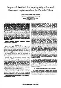
It is now evident that, every particle whose weight is less than I2 will appear only once with its weight unchanged, while every particle whose weight is greator than I2 will appear as many times as the integer part in the numerator of its weight with its weight equally divided amongst them. This procedure can be visualized in Fig. 1
3 I
2 I
1 I
(1)
w1 3
w2 2
w3 Discarded particles w4
The weights of the particles are updated as wki =
p(xk |z1:k ) i = wk−1 q(xk |z1:k )
p(zk |xik )
p(xik |xik−1 ) q(xik |z1:k )
w5
I X
wki δ(xk − xik )
w7
6
7
w8 1
(2)
where p(zk |xk ) is the likelihood. Then the weights are normalized and the posterior can be approximated as p(xk |z1:k ) ≈
w6
(3)
i=1
As the algorithm progresses, the discrepancy between the weights increases. This problem is called degeneracy [5]. One measure of the effciency in this context is the effective sample size [9], defined as 1 Ieff = PI (4) i 2 i=1 (wk ) such that Ieff � I, and low Ieff exhibits high degeneracy. The solution to degeneracy is to resample the particles with replacement. Whenever Ieff falls below a certain threshold [8], the particles with negligible weights should be replaced by those with higher weights. The idea is to eliminate particles that have small weights and replace them at the locations described by those that have larger weights [9, 12].
2
3
4
5
8
Fig. 1: Among the 8 particles, the first particle has a weight of 3.3 I and hence gets 3 copies each weighted at w31 = 1.1 . The second I particle has a weight of 2.8 and hence gets 2 copies each weighted at I w2 = 1.4 . The other particles’ weight is left unchanged since they 2 I are all less than I2 . The last 3 particles are discarded since we need only 8 particles Since only I reweighted particles are enough, the algorithm is terminated once I particles are created, and the others are discarded. This implies that we have deterministically replicated the particles and reweighted them based on ther individual weights. The weight of the discarded particles can be reallocated in one of the two following ways. Soft resampling - normalization: The weights can then be normalized as ai (8) bik = PI k i i=1 ak
4037
Soft resampling - redistributing the discarded weights: The weights of the discarded particles can be assigned to the retained particles in the following procedure. We first evaluate the total discarded weight as I X aspare = 1 − aik (9)
demonstrate this, we use the same example, now with a noise standard deviation of Σ = 2. The target appears in the 8th frame and maneuvers itself for 20 frames. Fig. 3 shows the number of frames taken to lock onto the target versus the number of particles, and it can be observed that our techniques lock faster with fewer particles.
No. of frames taken to lock onto the target
Normalizing would adjust the weights so that they sum to 1. When these weights are reused in the subsequent time step, they accurately describe the previous particles’ influence on the new particle set.
i=1
This weight is shared among the lower weight particles. To do this, we find the particle index p such that aspare + aIk + aI−1 + ... + aI−p ≤ aI−p−1 k k k
(10)
and each of the I − p particles starting from the Ith particle are reweighted as P aspare + Ii=I−p aik {bik }Ii=I−p = (11) p
18 16 14 12 10 8 6 4 3
4. EVALUATION
10
To demonstrate the validity of our techniques, we first test the softness of our methods. For this we used the PF based TBD numerical example described in chapter 11 of [4], which is also found in [14]. The observations now are 10×10 frames which are 2-D snapshots from a staring camera and all the results are averaged over 50 iterations. Fig. 2 shows the looseness of 1000 particles measured accordP
||xi −
PI
xi k
||2
i=1 I k ing to Ctight = versus the noise variance at the I camera with no target appearing for 30 frames. It can be observed that our techniques leave a looser cluster by the 30th frame.
4
10 No. of particles
Fig. 3: No, of frames taken from the appearance of a target to lock onto a target (i.e for the rms error to decrease to below 0.1) versus no. of particles. The target appears in the 8th frame and maneuvers for 20 frames. We now show that redistributing the weight of the discarded particles improves the accuracy of the scheme. Considering the same scheme where the target appears in the 8th frame and maneuvers for 20 frames, Fig. 4 shows the rms error versus the number of particles. It can be observed that the error is lower for the proposed methods.
4 3.5
0
10
2.5 2 1.5 1 0.5 0
rms error[m]
looseness of 1000 particles
3
multinomial residual stratified systematic Deterministic soft−redistributed soft−normalized Partial Aux. PF−systematic Aux. PF soft redistributed Aux. PF soft normalized
−0.5 0 10
1
10
−1
noise variance at the staring camera
10
3
10
Fig. 2: Tightness of 1000 particles versus noise variance. Particles keep searching for 30 frames with no target. The implementations are the PF with multinomial [3], residual [11], stratified [12], systematic [5] (implemented from [8]), deterministic (with the threshold chosen as I1 ) [13] and partial [9] (with the thresholds chosen as I2 and .9 ) resampling, auxiliary PF [6] with systematic resampling and I our proposed techniques on the PF and the auxiliary PF. The legend of this figure applies to Fig. 3, Fig. 4, Fig. 5 and Fig. 7 also. Since there is a loose cluster of particles to span the entire observation space, our techniques lock onto a new target much faster. To
4
10 No. of particles
Fig. 4: rms error versus number of particles. Noise variance at the camera is 4. The target appears in the 8th frame and maneuvers for 20 frames. It is a common practice to resample when the effective sample size Ieff drops below a threshold rather than at every time step [3, 5]. Fig. 5 shows rms error versus the Ieff threshold and it can be observed that our techniques perform accurately with a lower threshold, thereby allowing resampling less frequently, which in turn reduces the computational load.
4038
We finally test the simplicity of our approaches. Fig. 7 gives the computational time to complete the above simulation versus the number of particles. Our techniques are more simple since we do not need to model the birth and death of the particles.
1
2
10
0
10
600
700 800 Threshold for effective sample size
Computational time[s]
rms error[m]
10
1000
Fig. 5: rms error vs Ieff threshold for 1000 particles. Noise variance at the camera is 4. Target appears in the 8th frame and maneuvers for 20 frames.
0
10
−2
10
−4
10
0
10
10
8
8
y−position[m]
y−position[m]
We now demonstrate the complete TBD procedure and show that our resampler can be used directly in a classical PF, bypassing the need to model the birth and death of the targets. All the particles are alive all the time and tracks are initiated and terminated by observing the cluster looseness chosen to be 0.4. Fig. 6 shows the evolution of 5000 particles and the filter output. Our filter takes a little longer than the conventional TBD PF to declare absence of the target after the target has disappeared.
6
4
2
0 0
4 6 x−position[m]
8
6
4
0 0
10
2
10
8
8
6
4
2
0 0
8
10
4
2
2
4 6 x−position[m]
8
0 0
10
2
(c) 13th frame.
4 6 x−position[m]
(d) 24th frame. 10
8
8
y−position[m]
y−position[m]
10
6
10
6
4
2
0 0
8
(b) 8th frame.
10
y−position[m]
y−position[m]
(a) 5th frame.
4 6 x−position[m]
4 6 x−position[m]
(e) 28th frame.
8
10
4
5 4
x 10
Fig. 7: Computational time vs number of particles plot. Observations are 2-D snapshots from a 10×10 frame with a noise variance of 9. Results are averaged over 50 iterations of 30 frames each.
5. RELATION TO PRIOR WORK
6
6. CONCLUSION
4
2
2
2 3 No. of particles
Stochastic resampling techniques [3, 5, 11, 12] are extensively used in PFs to reduce particle degeneracy. However, they discard particles that may be gradually accumulating weight causing loss of potential information. These techniques also reset the weights equally [8, 16], with consequent loss of some of the information that could have been propagated to the next time step. Although deterministic resampling schemes overcome these limitations by allowing the information regarding the weights to survive the resampling process, the optimal resampling scheme of [13] does not reduce the variance among the weights and partial resampling [9] reweights the particles based on the number of dominant and negligible particles rather than on their individual weights. All these techniques are hard resamplers that are not feasible for direct use in TBD scenarios and necessitate modelling of the birth and death of particles [4, 14]. In this paper, we proposed two variants of a novel soft resampling method that achieves the simultaneous goals of maximising the retention of information over successive time steps, while minimizing the variance of the particle weights. The techniques can be used in a classical PF as a TBD PF making the process much simpler.
2
2
1
0 0
2
4 6 x−position[m]
8
10
(f) Actual vs estimate plot.
Fig. 6: Particle evolution of the PF using soft resampling. A target appears in the 8th frame and persists until the 24th frame. Noise variance at the camera 16. The blue line is the ground truth, magenta dots are the particles and the solid red line is the filter estimate.
In this paper, we proposed two approaches for soft resampling that can be used in a PF. Through simulations, we first demonstrated that our algorithms retain a looser cluster, which then aids in a faster lock when a target appears. We also demonstrated that our techniques exhibit higher tracking efficiency because of redistributing the weights of the discarded particles. We then demonstrated that our technique can be used in a classical PF for TBD applications and established that the computational load is reduced since we do not explicitly model particle birth and death.
4039
7. REFERENCES [1] R.P.S. Mahler, Statistical Multisource-Multitarget Information Fusion, vol. 685, Artech House Publishers, 2007. [2] W.M. Bolstad, Introduction to Bayesian statistics, WILEYINTERSCIENCE, 2004. [3] N.J. Gordon, D.J. Salmond, and A.F.M. Smith, “Novel approach to non-linear/non-Gaussian Bayesian state estimation,” in Proceedings IEE Radar and Signal Processing, 1993, vol. 140, pp. 107–113. [4] B. Ristic, S. Arulampalam, and N. Gordon, Beyond the Kalman Filter: Particle Filters for Tracking Applications, Artech House Publishers, 2004. [5] S. Arulampalam, S. Maskell, N. Gordon, and T. Clapp, “A tutorial on particle filters for online nonlinear/non-gaussian Bayesian tracking,” IEEE Transactions on Signal Processing, vol. 50, no. 2, pp. 174–188, 2002. [6] M.K. Pitt and N. Shephard, “Filtering via simulation: Auxiliary particle filters,” Journal of the American Statistical Association, pp. 590–599, 1999. [7] M. Orton and W. Fitzgerald, “A Bayesian approach to tracking multiple targets using sensor arrays and particle filters,” IEEE Transactions on Signal Processing, vol. 50, no. 2, pp. 216–223, 2002. [8] R. Douc and O. Capp´e, “Comparison of resampling schemes for particle filtering,” in Proceedings ISPA 4th International Symposium on Image and Signal Processing and Analysis, 2005, pp. 64–69. [9] M. Boli´c and S. and Hong P.M. Djuri´c, “Resampling algorithms for particle filters: A computational complexity perspective,” EURASIP Journal of Applied Signal Processing, vol. 2004, pp. 2267–2277, 2004. [10] D. Crisan, P. Del Moral, and T. Lyons, “Discrete filtering using branching and interacting particle systems,” Journal of Markov Processes and Related Fields, vol. 5, no. 3, pp. 293–318, 1999. [11] J. Liu and R. Chen, “Sequential Monte Carlo Methods for Dynamic Systems,” Journal of the American Statistical Association, vol. 93, pp. 1032–1044, 1998. [12] G. Kitagawa, “Monte Carlo filter and smoother for nonGaussian nonlinear state space models,” Journal of Computational and Graphical Statistics, pp. 1–25, 1996. [13] P. Fearnhead and P. Clifford, “On-line inference for hidden Markov models via particle filters,” Journal of the Royal Statistical Society: Series B (Statistical Methodology), vol. 65, pp. 887–899, 2003. [14] D.J. Salmond and H. Birch, “A particle filter for track-beforedetect,” in Proceedings IEEE American Control Conference, 2001, vol. 5, pp. 3755–3760. [15] M. Rollason and D. Salmond, “A particle filter for trackbefore-detect of a target with unknown amplitude,” in Proceedings IEE Target Tracking: Algorithms and Applications, 2001, vol. 1, pp. 14/1–14/4. [16] Jeroen D. Hol, Thomas B. Schon, and Fredrik Gustafsson, “On Resampling Algorithms for Particle Filters,” in Proceedings Nonlinear Statistical Signal Processing Workshop, 2006.
4040