SOFT ROUGH GRAPHS R. NOOR, I. IRSHAD, I. JAVAID*
Abstract. Soft set theory and rough set theory are mathematical tools to deal with uncertanitities. In [3], authors combined these concepts and introduced soft rough sets. In this paper, we introduce the concepts of soft rough graphs, vertex and edge induced soft rough graphs and soft rough trees. We define some products with examples in soft rough graphs.
1. Introduction and Preliminaries Many problems in engineering, computer science, social science, economics, medical science etc. have various uncertainties. To deal with these uncertainties, researchers have proposed a number of theories such as probability theory, fuzzy set theory, soft set theory, rough set theory, vague set theory etc. In [7], Molodtsov introduced the concept of soft sets. Soft set theory has applications in many different fields including the smoothness of functions, game theory, operational research, Perron integration, probability theory and measurement theory. Research on soft set theory is growing rapidly [1, 6, 8, 14]. In [9], Pawlak introduced the concept of rough sets. This theory deals with the approximation of an arbitrary subset of a universe by two definable or observable subsets called lower and upper approximations. It has been successfully applied to pattern recognition, machine learning, intelligent systems, inductive reasoning, image processing, knowledge discovery, signal analysis, decision analysis, expert systems and many other fields [10, 11, 12, 13]. In [3], authors introduced the concept of soft rough sets. Also, soft sets are combined with fuzzy sets and rough sets in [2]. The concept of rough soft group is defined in [4]. The concepts of soft graph and rough graph are introduced in [1] and [5] respectively. In this paper, we introduce the concept of soft rough graph, vertex and edge induced soft rough graph and soft rough trees. We study AND and OR operations in soft rough graphs. Also, we study the Cartesian, lexicographic and corona product and join of two soft rough graphs. Now we recall some notions related to soft sets and rough sets. Let U be the universe of discourse, R be an equivalence relation on U and P be the universe of Key words and phrases. Soft rough graph, vertex and edge induced soft rough graph, soft rough tree, Cartesian product of soft rough graphs, lexicographic product of soft rough graphs, corona product of soft rough graphs, join of soft rough graphs. ∗ Corresponding author:
[email protected]. 1
all possible parameters related to the objects in U . The power set of U is denoted by P (U ). Definition 1.1. [7]A pair F = (F, A) is called soft set over U , where A ⊆ P and F is a set valued mapping, F : A → P (U ). The ordered pair (U, P) is known as soft universe. Definition 1.2. [9]The pair (U, R) is called Pawlak approximation space. For X ⊆ U, R∗ (X ) = {x ∈ U : [x]R ⊆ U } R∗ (X ) = {x ∈ U : [x]R ∩ X 6= φ} are called lower and upper approximations of the set X . If R∗ (X ) = R∗ (X ) then X is said to be definable otherwise X is called rough set. Definition 1.3. [3] Let S = (U, F) be a soft approximation space. Based on S, the lower and upper soft rough approximations of X ⊆ U are defined by: F∗ (X ) = {u ∈ U : ∃ a ∈ A | u ∈ F(a) ⊆ X } and F∗ (X ) = {u ∈ U : ∃ a ∈ A | u ∈ F(a) and F(a) ∩ X 6= φ} respectively. If F∗ (X ) = F∗ (X ) then X is said to be soft definable otherwise X is called soft rough set, written as (F∗ (X ), F∗ (X ), A). A graph G = (V (G), E(G)) is a pair, where V (G) is the set of vertices and E(G) is the set of edges of G. When there is no ambiguity, we write G = (V, E). If two vertices x and y are adjacent in G, we write xy ∈ E(G). Two edges are said to be adjacent if they share a common vertex. A graph H is a subgraph of G if V (H) ⊆ V (G) and E(H) ⊆ E(G). The open neighborhood of v in G, N (v), is defined as N (v) = {u|uv ∈ E(G)} and N [v] = {v} ∪ N (v). The degree of v is defined as |N (v)|. A graph is called simple if it contains no loops or multiple edges. The distance between two vertices u, v of G, d(u, v), is the length of a shortest path between them. The diameter of a graph G, diam(G), is defined as diam(G) = max{d(u, v)|u, v ∈ V (G)}. ˜ Definition 1.4. [1] A graph G=(G, F, K, A) is called soft graph if it satisfies the following conditions: 1) G = (V, E) is a simple graph. 2) A is a non-empty set of parameters. 3) (F, A) is a soft set over V . 4) (K, A) is a soft set over E. 5) H(x) = (F(x), K(x)) is a subgraph of G for all x ∈ A. ˜ = hF, K, Ai = {H(x)| x ∈ A}. The set of all A soft graph can be represented by G soft graphs of G is denoted by SG(G). 2
2. Soft Rough Graphs Let S = (U, F) be a soft approximation space, A ⊆ P be any non-empty subset of parameters and X ⊆ U be any non-empty subset of U. Let (F∗ (X ), F∗ (X ), A) be a soft rough set over V with its lower and upper approximations defined as: F∗ (X ) = {u ∈ U : ∃ a ∈ A | u ∈ F(a) ⊆ X } and F∗ (X ) = {u ∈ U : ∃ a ∈ A | u ∈ F(a) and F(a) ∩ X 6= φ} respectively, where (F, A) be a soft set over V with F : A → P (V ) defined as F(x) = {y ∈ V : xRy}. Let (K∗ (X ), K∗ (X ), A) be a soft rough set over E with its lower and upper approximations defined as: K∗ (X ) = {e ∈ E : ∃ a ∈ A | e ∈ K(a) ⊆ X } and K∗ (X ) = {e ∈ E : ∃ a ∈ A | e ∈ K(a) and K(a) ∩ X 6= φ} respectively, where (K, A) be a soft set over E with K : A → P (E) defined as: K(x) = {e ∈ E | e ⊆ F(x)}. ˜ = (G, F∗ , K∗ , F∗ , K∗ , A, X ) is called soft rough graph if Definition 2.1. A graph G it satisfies the following conditions: 1) G = (V, E) is a simple graph. 2) A be a non-empty set of parameters. 3) X be any non-empty subset of U. 4) (F∗ (X ), F∗ (X ), A) be a soft rough set over V . 5) (K∗ (X ), K∗ (X ), A) be a soft rough set over E. 6) H∗ (X ) = (F∗ (X ), K∗ (X )) and H∗ (X ) = (F∗ (X ), K∗ (X )) are subgraphs of G. A soft rough graph can be represented by ˜ = hF∗ , K∗ , F∗ , K∗ , A, X i = {H∗ (X ), H∗ (X )}. G The set of all soft rough graphs of G is denoted by SRG(G). ˜ = hF∗ , K∗ , F∗ , K∗ , A, X i is said to be lower Definition 2.2. A soft rough graph G vertex induced graph if H∗ (X ) = (F∗ (X ), K∗ (X )) = hF∗ (X )i for X ⊆ V, upper vertex induced graph if H∗ (X ) = (F∗ (X), K∗ (X )) = hF∗ (X )i for X ⊆ V, lower edge induced graph if H∗ (X ) = (F∗ (X ), K∗ (X )) = hK∗ (X )i for X ⊆ V, 3
upper edge induced graph if H∗ (X ) = (F∗ (X ), K∗ (X )) = hK∗ (X )i for X ⊆ V. Example 2.3. Let G = (V, E) be a graph with V = {v1 , v2 , v3 , v4 , v5 } and E = {e1 , e2 , e3 , e4 , e5 , e6 , e7 , e8 , e9 } as shown in FIGURE 1. Let A = {v1 , v3 } be the set v1 e5 v5
e1 e6 e7
e8
e4 v4
v2
e3
e2 v3
Figure 1 of parameters and F : A → P (V ) is defined as F(x) = {y ∈ V : xRy ⇔ y ∈ N (x)}. Then F(v1 ) = {v2 , v5 }, F(v3 ) = {v2 , v4 , v5 }. Let X = {v1 , v2 , v5 } be a subset of V. The lower and upper soft rough approximations over V are as follows: F∗ (X ) = {v2 , v5 }, F∗ (X ) = {v2 , v4 , v5 } respectively. The lower and upper soft rough approximations over E are as follows: K∗ (X ) = {e6 }, K∗ (X ) = {e4 , e6 , e8 } respectively.
Now H∗ (X ) = (F∗ (X ), K∗ (X )) = ({v2 , v5 }, {e6 }) and H∗ (X ) = v5 v5
e6
v2
e4
H (X) *
e6
v2
e5 v4
H*(X)
Figure 2 (F∗ (X ), K∗ (X )) = ({v2 , v4 , v5 }, {e4 , e6 , e8 }) as shown in FIGURE 2. Definition 2.4. Let G˜1 = hF1∗ , K1∗ , F∗1 , K1∗ , A, X i and G˜2 = hF2∗ , K2∗ , F∗2 , K2∗ , B, X i be two soft rough graphs of G. Then G˜2 is called soft rough subgraph of G˜1 if the following conditions hold: 1) B ⊆ A. 4
2) H2∗ (X ) = (F2∗ (X ), K2∗ (X )) is a subgraph of H1∗ (X ) = (F1∗ (X ), K1∗ (X )). 3) H2∗ (X ) = (F∗2 (X ), K2∗ (X )) is a subgraph of H1∗ (X ) = (F∗1 (X ), K1∗ (X )). Example 2.5. Let G = (V, E) be a graph with V = {v1 , v2 , v3 , v4 , v5 , v6 .v7 } and E = {e1 , e2 , e3 , e4 , e5 , e6 , e7 , e8 , e9 , e10 , e11 } as shown in FIGURE 3. Let B = {v2 , v4 } v2 e9 e10
v7
v1
v3
e2
e1 e11
v6
e8
e5
e3
e7
e6
v4
e4
v5
Figure 3 be the set of parameters and F2 : B → P (V ) is defined as F2 (x) = {y ∈ V : xRy ⇔ y ∈ N (x)}. Then F2 (v2 ) = {v1 , v3 , v6 }, F2 (v4 ) = {v3 , v5 , v6 }. Let X = {v1 , v3 , v6 } be a subset of V. The lower and upper soft rough approximations over V are as follows: F2∗ (X ) = {v1 , v3 , v6 }, F∗2 (X ) = {v1 , v3 , v5 , v6 } respectively. The lower and upper soft rough approximation over E are as follows: K2∗ (X ) = {e8 }, K2∗ (X ) = {e6 , e8 } respectively. As H2∗ (X ), H2∗ (X ) are shown in FIGURE 4, hence G˜2 = {H2∗ (X ), H2∗ (X )} be the soft rough graph of G. Let A = {v2 , v3 , v4 } be the set of parameters such that v3 v3 e8 H2*(X)
e8
v1
v1
e5
v6
v6 e6 v5
H2* (X)
Figure 4 B ⊆ A. Let F1 : A → P (V ) defined as F1 (x) = {y ∈ V : xRy ⇔ y ∈ N (x)}. Then F1 (v2 ) = {v1 , v3 , v6 }, F1 (v4 ) = {v3 , v5 , v6 }, F1 (v3 ) = {v2 , v4 , v6 }. The lower and upper soft rough approximations over V are as follows: F1∗ (X ) = {v1 , v3 , v6 }, F∗1 (X ) = {v1 , v2 , v3 , v4 , v5 , v6 } 5
respectively. The lower and upper soft rough approximations over E are as follows: K1∗ (X ) = {e8 }, K1∗ (X ) = {e1 , e2 , e3 , e4 , e5 , e6 , e7 , e8 , e9 } respectively. As H1∗ (X ), H1∗ (X ) are shown in FIGURE 5, hence G˜1 = {H1∗ (X ), H1∗ (X )} be the soft rough graph of G. Since B ⊆ A, H2∗ (X ) is a subgraph of H1∗ (X ) and v2
v3
v1 e8
e9
v1 e1
e6
e5
v6
e2
v
v3 e8
v6 e 7
e3 v4
e4
5
H1*(X)
H1*(X)
Figure 5 H2∗ (X ) is a subgraph of H1∗ (X ). So, G˜2 is a soft rough subgraph of G˜1 . Theorem 2.6. Let G˜1 = hF1∗ , F∗1 , K1∗ , K1∗ , A, X i and G˜2 = hF2∗ , F∗2 , K2∗ , K2∗ , B, X i be two soft rough graphs of G. Then G˜2 is a soft rough subgraph of G˜1 if and only if F2∗ (X ) ⊆ F1∗ (X ), F∗2 (X ) ⊆ F∗1 (X ), K2∗ (X ) ⊆ K1∗ (X ) and K2∗ (X ) ⊆ K1∗ (X ). Proof. Given G˜1 and G˜2 be two soft rough graphs of G. Suppose G˜2 is a soft rough subgraph of G˜1 . Then by the definition of soft rough subgraph: 1) B ⊆ A. 2) H2∗ (X ) = (F2∗ (X ), K2∗ (X )) is a subgraph of H1∗ (X ) = (F1∗ (X ), K1∗ (X )). 3) H2∗ (X ) = (F∗2 (X ), K2∗ (X )) is a subgraph of H1∗ (X ) = (F∗1 (X ), K1∗ (X )). Since H2∗ (X ) is a subgraph of H1∗ (X ) and H2∗ (X ) is a subgraph of H1∗ (X ). Thus F2∗ (X ) ⊆ F1∗ (X ), K2∗ (X ) ⊆ K1∗ (X ), F∗2 (X ) ⊆ F∗1 (X ) and K2∗ (X ) ⊆ K1∗ (X ). Conversely suppose that F2∗ (X ) ⊆ F1∗ (X ), K2∗ (X ) ⊆ K1∗ (X ), F∗2 (X ) ⊆ F∗1 (X ) and K2∗ (X ) ⊆ K1∗ (X ). Since G˜1 is a soft rough graph of G, H1∗ (X ) and H1∗ (X ) be the subgraphs of G. Since G˜2 is a soft rough graph of G, H2∗ (X ) and H2∗ (X ) be subgraphs of G. Thus H2∗ (X ) = (F2∗ (X ), K2∗ (X )) is a subgraph of H1∗ (X ) = (F1∗ (X ), K1∗ (X )) and H2∗ (X ) = (F∗2 (X ), K2∗ (X )) is a subgraph of H1∗ (X ) = (F∗1 (X ), K1∗ (X )). Hence G˜2 is a soft rough subgraph of G˜1 . ¤ ˜ = hF∗ , K∗ , F∗ , K∗ , A, X i be a soft rough graph of G. Then G ˜ Definition 2.7. Let G is called a soft rough tree if H∗ (X ) and H∗ (X ) are trees. Example 2.8. Let G = (V, E) be a graph with V = {v1 , v2 , v3 , v4 , v5 } and E = {e1 , e2 , e3 , e4 , e5 } as shown in FIGURE 6. Let A = {v1 , v2 } be the set of parameters and F : A → P (V ) is defined as F(x) = {y : xRy ⇔ d(x, y) = diam(G)}. 6
v1 e1
e5 v5
v2 e4
e2
v4
e3
v3
Figure 6 Then F(v1 ) = {v3 , v4 }, F(v2 ) = {v4 , v5 }. Let X = {v2 , v3 , v4 } then the lower and upper soft rough approximations over V are as follows: F∗ (X) = {v3 , v4 }, F∗ (X) = {v3 , v4 , v5 }, respectively. The lower and upper soft rough approximations over E are as follows: K∗ (X) = {e3 }, K∗ (X) = {e3 , e4 }, ˜ is a respectively. As shown in FIGURE 7, H∗ (X ) and H∗ (X ) are trees. Hence G soft rough tree. v3 e3
v3 v4
e3 e4
v4
v5
H* (X)
H*(X)
Figure 7 ˜ of T is a soft rough Lemma 2.9. Let T be a tree. Then any soft rough graph G tree. ˜ = hF∗ , F∗ , K∗ , K∗ , A, X i of Proof. Since T is a tree so for any soft rough graph G ∗ T , H∗ (X ) and H (X ) are trees. ¤ 7
Note that converse of above Lemma is not true in general. As in Example 2.8, H∗ (X ) and H∗ (X ) are trees but G is a cycle of order 5. Remark 2.10. Let G˜1 = hF1∗ , F∗1 , K1∗ , K1∗ , A, X i be a soft rough tree of G. If G˜2 = hF2∗ , F∗2 , K2∗ , K2∗ , B, Yi is a soft rough subgraph of G˜1 then G˜2 is a soft rough tree of G. Definition 2.11. Let G˜1 = hF1∗ , F∗1 , K1∗ , K1∗ , A, X i and G˜2 = hF2∗ , F∗2 , K2∗ , K2∗ , B, Yi be two soft rough graphs of G. Then AND operation of G˜1 and G˜2 is denoted by G˜1 f G˜2 and is defined as G˜1 f G˜2 = hF∗ , K∗ , F∗ , K∗ , A × B, X × Yi, where F∗ (X × Y) = F1∗ (X ) ∩ F2∗ (Y), K∗ (X × Y) = K1∗ (X ) ∩ K2∗ (Y), F∗ (X × Y) = F∗1 (X ) ∩ F∗2 (Y) and K∗ (X × Y) = K1∗ (X ) ∩ K2∗ (Y). Definition 2.12. Let G˜1 = hF1∗ , F∗1 , K1∗ , K1∗ , A, X i and G˜2 = hF2∗ , F∗2 , K2∗ , K2∗ , B, Yi be two soft rough graphs of G. Then OR operation of G˜1 and G˜2 is denoted by G˜1 g G˜2 and is defined as G˜1 g G˜2 = hF∗ , K∗ , F∗ , K∗ , A × B, X × Yi, where F∗ (X × Y) = F1∗ (X ) ∪ F2∗ (Y), K∗ (X × Y) = K1∗ (X ) ∪ K2∗ (Y), F∗ (X × Y) = F∗1 (X ) ∪ F∗2 (Y) and K∗ (X × Y) = K1∗ (X ) ∪ K2∗ (Y). Example 2.13. Let G = (V, E) be a graph with V = {v1 , v2 , v3 , v4 , v5 } and E = {e1 , e2 , e3 , e4 , e5 , e6 , e7 , e8 } as shown in FIGURE 8. Let A = {v2 , v5 } be the set of parameters. We define an approximate function F1 : A → P (V ) as F1 (x) = {y ∈ V : xRy ⇔ y ∈ N (x)}. Then F1 (v2 ) = {v1 , v3 , v5 }, F1 (v5 ) = {v1 , v2 , v3 , v4 }. Let X = {v1 , v2 , v3 , v5 } be the e2
v4
v3
e8
e3 e6
e5 v1
e7
v5
e1
e4
v2
Figure 8 subset of V. The lower and upper soft rough approximations over V are as follows: F1∗ (X ) = {v1 , v3 , v5 }, F∗1 (X ) = {v1 , v2 , v3 , v4 , v5 } respectively. The lower and upper soft rough approximations over E are as follows: K1∗ (X ) = {e5 , e7 }, K1∗ (X ) = {e1 , e2 , e3 , e4 , e5 , e6 , e7 , e8 } 8
˜ 1 = {H1∗ (X ), H∗ (X )} be the soft rough graph of G. Let B = respectively. So, G 1 {v3 , v4 } be the set of parameters and Y = {v1 , v2 , v4 , v5 } be a subset of V. We define an approximate function F2 : B → P (V ) as F2 (x) = {y ∈ V : xRy ⇔ y ∈ N (x)}. Then F2 (v3 ) = {v2 , v4 , v5 }, F2 (v4 ) = {v1 , v3 , v5 }. The lower and upper soft rough approximations over V are as follows: F2∗ (Y) = {v2 , v4 , v5 }, F∗2 (Y) = {v1 , v3 , v4 , v5 } respectively. The lower and upper soft rough approximations over E are as follows: K2∗ (Y) = {e6 , e8 }, K2∗ (Y) = {e1 , e2 , e5 , e7 , e8 } ˜ 2 = {H2∗ (Y), H∗ (Y)} be the soft rough graph of G. Now the AND respectively. So, G 2 ˜ 1 and G ˜ 2 is given as follows: operation of G F∗ (X × Y) = F1∗ (X ) ∩ F2∗ (Y) = {v5 }, K∗ (X × Y) = K1∗ (X ) ∩ K2∗ (Y) = ∅, F∗ (X × Y) = F∗1 (X ) ∩ F∗2 (Y) = {v1 , v3 , v4 , v5 }, K∗ (X × Y) = K1∗ (X ) ∩ K2∗ (Y) = {e1 , e2 , e5 , e7 , e8 }. ˜ 1 and G ˜ 2 is given as follows: Now the OR operation of G F∗ (X × Y) = F1∗ (X ) ∪ F2∗ (Y) = {v1 , v2 , v3 , v4 , v5 }, K∗ (X × Y) = K1∗ (X ) ∪ K2∗ (Y) = {e5 , e6 , e7 , e8 }, F∗ (X × Y) = F∗1 (X ) ∪ F∗2 (Y) = {v1 , v2 , v3 , v4 , v5 }, K∗ (X × Y) = K1∗ (X ) ∪ K2∗ (Y) = {e1 , e2 , e3 , e4 , e5 , e6 , e7 , e8 }. Theorem 2.14. Let G˜1 = hF1∗ , F∗1 , K1∗ , K1∗ , A, X i and G˜2 = hF2∗ , F∗2 , K2∗ , K2∗ , B, Yi be two soft rough graphs of G such that F1∗ (X ) ∩ F2∗ (Y) 6= ∅, F∗1 (X ) ∩ F∗2 (Y) 6= ∅, K1∗ (X ) ∩ K2∗ (Y) 6= ∅ and K1∗ (X ) ∩ K2∗ (Y) 6= ∅. Then their AND operation is a soft rough graph of G. Proof. Since G˜1 is a soft rough graph of G, H1∗ (X ) = (F1∗ (X ), K1∗ (X )) and H1∗ (X ) = (F∗1 (X ), K1∗ (X )) are subgraphs of G. Since G˜2 is a soft rough graph of G, H2∗ (X ) = (F2∗ (X ), K2∗ (X )) and H2∗ (X ) = (F∗2 (X ), K2∗ (X )) are subgraphs of G. Let (F∗ (X × Y), K∗ (X × Y)) = (F1∗ (X ) ∩ F2∗ (Y), K1∗ (X ) ∩ K2∗ (Y)) and (F∗ (X × Y), K∗ (X × Y)) = (F∗1 (X ) ∩ F∗2 (Y), K1∗ (X ) ∩ K2∗ (Y)). Since (F1∗ (X ), K1∗ (X )), (F2∗ (Y), K2∗ (Y)), (F∗1 (X ), K1∗ (X )),, (F∗2 (Y), K2∗ (Y)) be the subgraphs of G and by assumption F1∗ (X )∩ F2∗ (Y) 6= ∅, F∗1 (X ) ∩ F∗2 (Y) 6= ∅, K1∗ (X ) ∩ K2∗ (Y) 6= ∅ and K1∗ (X ) ∩ K2∗ (Y) 6= ∅. So, (F∗ (X × Y), K∗ (X × Y)) and (F∗ (X × Y), K∗ (X × Y)) are subgraphs of G. Hence G˜1 f G˜2 be a soft rough graph of G. ¤ Theorem 2.15. Let G˜1 = hF1∗ , F∗1 , K1∗ , K1∗ , A, X i and G˜2 = hF2∗ , F∗2 , K2∗ , K2∗ , B, Yi be two soft rough graphs of G such that F1∗ (X ) ∪ F2∗ (Y) 6= ∅, F∗1 (X ) ∪ F∗2 (Y) 6= ∅, K1∗ (X ) ∪ K2∗ (Y) 6= ∅ and K1∗ (X ) ∪ K2∗ (Y) 6= ∅. Then their OR operation is a soft rough graph of G. Proof. The proof is obvious.
¤ 9
The Cartesian product of two graphs G1 = (V1 , E1 ) and G2 = (V2 , E2 ) is a graph G = G1 × G2 = (V, E) where the vertex set of G is the cartesian product of V1 and V2 and edge set is defined as E = {(u, v), (u, w) | u ∈ V1 , (v, w) ∈ E2 } ∪ {(y, x), (z, x) | x ∈ V2 , (y, z) ∈ E1 }. Definition 2.16. Let G˜1 = hF1∗ , F∗1 , K1∗ , K1∗ , A, X i and G˜2 = hF2∗ , F∗2 , K2∗ , K2∗ , B, Yi be soft rough graphs of G1 and G2 respectively. The Cartesian product of G˜1 and G˜2 is denoted by G˜1 n G˜2 and is defined as G˜1 n G˜2 = hL∗ , L∗ , A × B, X × Yi, where L∗ (X × Y) = H1∗ (X ) × H2∗ (Y), L∗ (X × Y) = H1∗ (X ) × H2∗ (Y) and H1∗ (X ) × H2∗ (Y), H1∗ (X ) × H2∗ (Y) be the Cartesian product of subgraphs H1∗ (X ), H2∗ (Y), H1∗ (X ) and H2∗ (Y). The lexicographic product of two graphs G1 and G2 is denoted by G1 ◦ G2 , is the graph with vertex set V (G1 ) × V (G2 ) = {(a, v) | a ∈ V (G1 ) and v ∈ V (G2 )}, where (a, v) is adjacent to (b, w) whenever ab ∈ E(G1 ) or a = b and vw ∈ E(G2 ). For any vertex a ∈ V (G1 ) and b ∈ V (G2 ), we define the vertex set G2 (a) = {(a, v) ∈ V (G1 ◦ G2 ) | v ∈ V (G2 )} and G1 (b) = {(v, b) ∈ V (G1 ◦ G2 ) | v ∈ V (G1 )}. Definition 2.17. Let G˜1 = hF1∗ , F∗1 , K1∗ , K1∗ , A, X i and G˜2 = hF2∗ , F∗2 , K2∗ , K2∗ , B, Yi be soft rough graphs of G1 and G2 respectively. The lexicographic product of G˜1 and G˜2 is denoted by G˜1 ¯ G˜2 and is defined as G˜1 ¯ G˜2 = hN∗ , N ∗ , A × B, X × Yi, where N∗ (X × Y) = H1∗ (X ) ◦ H2∗ (Y), N ∗ (X × Y) = H1∗ (X ) ◦ H2∗ (Y) and H1∗ (X ) ◦ H2∗ (Y), H1∗ (X ) ◦ H2∗ (Y) be the lexicographic product of subgraphs H1∗ (X ), H2∗ (Y), H1∗ (X ) and H2∗ (Y). The join of two graphs G1 = (V1 , E1 ) and G2 = (V2 , E2 ) is denoted by G1 + G2 and is defined as the union of graphs obtained by joining each vertex v ∈ V1 to all vertices w ∈ V2 , i.e G1 + G2 = (V1 ∪ V2 , E1 ∪ E2 ∪ E), where E is the set of all edges joining the vertices of V1 and V2 . Definition 2.18. Let G˜1 = hF1∗ , F∗1 , K1∗ , K1∗ , A, X i and G˜2 = hF2∗ , F∗2 , K2∗ , K2∗ , B, Yi be soft rough graphs of G1 and G2 respectively. The join of G˜1 and G˜2 is denoted by G˜1 ⊕ G˜2 and is defined as G˜1 ⊕ G˜2 = hD∗ , D∗ , A × B, X × Yi, where D∗ (X × Y) = H1∗ (X ) + H2∗ (Y), D∗ (X × Y) = H1∗ (X ) + H2∗ (Y) and H1∗ (X ) + H2∗ (Y), H1∗ (X )+H2∗ (Y) be the join of subgraphs H1∗ (X ), H2∗ (Y), H1∗ (X ) and H2∗ (Y). The corona product of two graphs G1 = (V1 , E1 ) and G2 = (V2 , E2 ) with |G1 | = n1 and |G2 | = n2 is denoted by G1 ¦ G2 and is defined as the graph obtained from G1 10
and G2 by taking one copy of G1 and n1 copies of G2 and joining by an edge each vertex from the ith-copy of G2 with the ith-vertex of G1 . Definition 2.19. Let G˜1 = hF1∗ , F∗1 , K1∗ , K1∗ , A, X i and G˜2 = hF2∗ , F∗2 , K2∗ , K2∗ , B, Yi be soft rough graphs of G1 and G2 respectively. The corona product of G˜1 and G˜2 is denoted by G˜1 } G˜2 and is defined as G˜1 } G˜2 = hM∗ , M∗ , A × B, X × Yi, where M∗ (X × Y) = H1∗ (X ) ¦ H2∗ (Y), M∗ (X × Y) = H1∗ (X ) ¦ H2∗ (Y) and H1∗ (X ) ¦ H2∗ (Y), H1∗ (X ) ¦ H2∗ (Y) be the corona product of subgraphs H1∗ (X ), H2∗ (Y), H1∗ (X ) and H2∗ (Y). Example 2.20. Let G1 and G2 be the graphs given in FIGURE 9. Let V1 = {a, b, c, d, e} and V2 = {f, g, h, k} be the set of vertices of G1 and G2 respectively. Let E1 = {e1 , e2 , e3 , e4 } and E2 = {t1 , t2 , t3 } be the set of edges of G1 and G2 respectively. Let A = {d, e} ⊆ V1 and B = {g, k} ⊆ V2 be the set of parameters. We define approximate functions F1 : A → P (V1 ) and F2 : B → P (V2 ) by F1 (x) = {y ∈ V1 : xRy ⇔ y ∈ N (x)}, F2 (x) = {y ∈ V2 : xRy ⇔ y ∈ N [x]}. Then F1 (e) = {d}, F1 (d) = {c, e}, F2 (g) = {f, g, h}, F2 (k) = {h, k}. Let X = a f
e1
t1
b g e2
G1
t2
c h
e3
G2
t3
d k
e4
e
Figure 9 {b, c, d} ⊆ V1 and Y = {h, k} ⊆ V2 . The lower and upper vertex approximations with respect to X and Y are given as follows: F1∗ (X ) = {d}, F∗1 (X ) = {c, e, d}, F2∗ (Y) = {k, h}, F∗2 (Y) = {f, g, h, k}. The lower and upper edge approximations with respect to X and Y are given as follows: K1∗ (X ) = {e3 , e4 }, K1∗ (X ) = ∅, K2∗ (Y) = {t1 , t2 , t3 }, K2∗ (Y) = {t3 }. 11
f t1
c g
e3
h
t2
d d
t3
e4
H1
(X)
*
h t3
e
k
k
H1*(X)
H 2 *(X)
H2*(X)
Figure 10 FIGURE 10 shows H1∗ (X ) = (F1∗ (X ), K1∗ (X )), H2∗ (Y) = (F2∗ (Y), K2∗ (Y)), H1∗ (X ) = ˜ 1 and G ˜ 2 are the soft rough graphs. (F∗1 (X ), K1∗ (X )), H2∗ (Y) = (F∗2 (Y), K2∗ (Y)). So, G FIGURE 11 shows the subgraphs L∗ and L∗ . FIGURE 12 shows the subgraphs N∗ (d, f)
(e, h)
(c, f)
(c, g) (d, h)
(d, g)
(e, g)
(d, k)
L
*
(c, h)
(d, h)
(e, h)
(e, k)
(c, k) (d, k)
L*
Figure 11. Subgraphs L∗ and L∗ and N ∗ . FIGURE 13 shows the subgraphs D∗ and D∗ . FIGURE 14 shows the subgraphs M∗ and M∗ . Theorem 2.21. Let G˜1 = hF1∗ , F∗1 , K1∗ , K1∗ , A, X i and G˜2 = hF2∗ , F∗2 , K2∗ , K2∗ , B, Yi be soft rough graphs of G1 and G2 respectively. Let L be the Cartesian product of G1 and G2 then G˜1 n G˜2 = hL∗ , L∗ , A × B, X × Y i is a soft rough graph of L. Proof. The Cartesian product of two soft rough graphs G˜1 and G˜2 is defined as G˜1 n G˜2 = hL∗ , L∗ , A × B, X × Yi, where L∗ (X × Y) = H1∗ (X ) × H2∗ (Y) and L∗ (X × Y) = H1∗ (X ) × H2∗ (Y). Since G˜1 is a soft rough graph of G1 , H1∗ (X ) and H1∗ (X ) are subgraphs of G1 , and G˜2 is a soft rough graph of G2 , H2∗ (Y) and H2∗ (Y) are subgraphs of G2 . So, L∗ (X × Y) and L∗ (X × Y) being the Cartesian product of two subgraphs are subgraphs of L. Hence G˜1 n G˜2 is a soft rough graph of L. ¤ 12
(d, f)
(c, f)
(d, h)
(c, g)
(d, g)
(c, h)
(d, h)
(e, f)
(e, g)
(d, k)
N *
(e, h)
(c,k)
(e,k) (d, k)
N*
Figure 12. Subgraphs N∗ and N ∗ f c
k
g
d
d h
h
D *
e k
D*
Figure 13. Subgraphs D∗ and D∗ g
f h
k
h
f
f d
g
g c
d
h
h
k
M *
e
k
M*
k
Figure 14. Subgraphs M∗ and M∗ Theorem 2.22. Let G˜1 = hF1∗ , F∗1 , K1∗ , K1∗ , A, X i and G˜2 = hF2∗ , F∗2 , K2∗ , K2∗ , B, Yi be soft rough graphs of G1 and G2 respectively. Let N be the lexicographic product of G1 and G2 then G˜1 ¯ G˜2 = hN∗ , N ∗ , A × B, X × Yi is a soft rough graph of N . Proof. The lexicographic product of two soft rough graphs G˜1 and G˜2 is G˜1 ¯ G˜2 = hN∗ , N ∗ , A × B, X × Yi, where N∗ (X × Y) = H1∗ (X ) ◦ H2∗ (Y) and N ∗ (X × Y) = H1∗ (X ) ◦ H2∗ (Y). Since G˜1 is a soft rough graph of G1 , H1∗ (X ) and H1∗ (X ) are 13
subgraphs of G1 . Since G˜2 is a soft rough graph of G2 , H2∗ (Y) and H2∗ (Y) are subgraphs of G2 . So, N∗ (X × Y) and N ∗ (X × Y) being the lexicographic product of two subgraphs are subgraphs of N . Hence G˜1 ¯ G˜2 is a soft rough graph of N . ¤ Theorem 2.23. Let G˜1 = hF1∗ , F∗1 , K1∗ , K1∗ , A, X i and G˜2 = hF2∗ , F∗2 , K2∗ , K2∗ , B, Yi be soft rough graphs of G1 and G2 respectively. Let D be the join of G1 and G2 then G˜1 ⊕ G˜2 = hD∗ , D∗ , A × B, X × Yi is a soft rough graph of N . Proof. The join of two soft rough graphs G˜1 and G˜2 is G˜1 ⊕G˜2 = hD∗ , D∗ , A×B, X × Yi, where D∗ (X × Y) = H1∗ (X ) + H2∗ (Y) and D∗ (X × Y) = H1∗ (X ) + H2∗ (Y). Since G˜1 is a soft rough graph of G1 , H1∗ (X ) and H1∗ (X ) are subgraphs of G1 . Since G˜2 is a soft rough graph of G2 , H2∗ (Y) and H2∗ (Y) are subgraphs of G2 . So, D∗ (X × Y) and D∗ (X × Y) being the join of two subgraphs are subgraphs of N . Hence G˜1 ⊕ G˜2 is a soft rough graph of N . ¤ Theorem 2.24. Let G˜1 = hF1∗ , F∗1 , K1∗ , K1∗ , A, X i and G˜2 = hF2∗ , F∗2 , K2∗ , K2∗ , B, Yi be soft rough graphs of G1 and G2 respectively. Let M be the corona product of G1 and G2 then G˜1 } G˜2 = hM∗ , M∗ , A × B, X × Yi is a soft rough graph of M. Proof. The corona product of two soft rough graphs G˜1 and G˜2 is G˜1 } G˜2 = hM∗ , M∗ , A×B, X ×Yi, where M∗ (X ×Y) = H1∗ (X )¦H2∗ (Y) and M∗ (X × Y) = H1∗ (X ) ¦ H2∗ (Y). Since G˜1 is a soft rough graph of G1 , H1∗ (X ) and H1∗ (X ) are subgraphs of G1 . Since G˜2 is a soft rough graph of G2 , H2∗ (Y) and H2∗ (Y) are subgraphs of G2 . So, M∗ (X × Y) and M∗ (X × Y) being the corona product of two subgraphs are subgraphs of N . Hence G˜1 } G˜2 is a soft rough graph of M. ¤ References [1] M. Akram, and S. Nawaz, Operations on soft graphs, Fuzzy Inf. Eng., 7(2015), 423-449. [2] F. Feng, C. Li, B. Davvaz and M. I. Ali, Soft sets combined with fuzzy sets and rough sets: a tentative approach, Soft Comput., 14(2010), 899-911. [3] F. Feng, X. Liu, V. L. Fotea and Y. B. Jun, Soft sets and soft rough sets, Inform. Sci., 181(2011), 1125-1137. [4] J. Ghosh and T. K. Samanta, Rough Soft Sets and Rough Soft Groups, J. Hyperstructures, 2(1)(2013), 18-29. [5] H. Tong, L. Chang-jing and S. KAi-quan, Rough graph and its structure, J. Shandong Univ., 41(6)(2006), 46-50. [6] P. K. Maji, R. Biswas, and A. R. Roy, Soft set theory, Comput. Math. Appl., 45.(2003), 555-562. [7] D. Molodtsov, Soft set theory, first results, Comput. Math. Appl., 37(1999), 19-31. [8] E. K. R. Nagarajan and G. Meenambigai, An application of soft sets to lattices, Kragujevac J. Math., 35(1)(2011), 75-87. [9] Z. Pawlak, Rough sets, Int. J. Comput. Inform. Sci., 11(1982), 41-356. [10] Z. Pawlak, Rough Sets: Theoretical Aspects of Reasoning about Data, Kluwer Academic Publishers, Dordrecht, 1991. [11] Z. Pawlak, A. Skowron, Rudiments of rough sets, Inform. Sci., 177(2007), 3-27. 14
[12] Z. Pawlak, A. Skowron, Rough sets: some extensions, Inform. Sci., 177 (2007), 28-40. [13] Z. Pawlak, A. Skowron, Rough sets and Boolean reasoning, Inform. Sci., 177(2007), 41-73. [14] R. K. Thumbakara, and B. George, Soft graphs, Gen. Math. Notes, 21(2)(2014), 75-86. Centre for advanced studies in Pure and Applied Mathematics, Bahauddin Zakariya University Multan, Pakistan. Email:
[email protected],
[email protected],
[email protected]
15