paradigm as genuine enhancements to the construc- .... A major advantage of the minimalist approach of ..... and Anal~ysis Using Sigma for Windows, Boyd and.
Proceedings of the 1996 Winter Sirnulation Conference ed. J. M. Charnes, D. J. Morrice, D. T. Brunner, and J. J. Snrain
MODELING WITH EVENT GRAPHS Arnold H. Buss Operations Research Department Naval Postgraduate School Monterey, CA 93943-5000, U.S.A.
ABSTRACT
some examples. Following that, we describe the enhanced features and show examples of their use.
Event Graphs are a way of graphically representing discrete-event simulation models. Also known as "Simulation Graphs," they have a minimalist design, with a single type of node and two types of edges with up to three options. Despite this simplicity, Event Graphs are extremely powerful. The Event Graph is the only graphical paradigm that directly models the event list logic. There are no limitations to the ability of Event Graphs to create a simulation model for any circumstance. Their simplicity, together with their extensibility, make them an ideal tool for rapid construction and prototyping of simulation models. In this paper we will demonstrate the ability of Event Graphs to leverage simple models into more complex ones with very few additional features.
1
2
BASICS OF EVENT GRAPH MODELS
We assume the reader is familiar with the basic concepts of discrete event simulation (see any introductory text such as Law and Kelton 1991), so we will only briefly review the components. Two fundamental components of a discrete event sinlulation model are a set of state variables, and a set of events. The model emulates the system being studied by producing state trajectories, that is, time plots of the values of the system's state variables. Measures of performance are determined as statistics of these state trajectories. Discrete event models have state trajectories that are piecewise constant. Events are the points in time at which at least one state variable changes value. It is important to note that an event is an instantaneous occurrence in the discrete event model. No simulated time passes when an event occurs; simulated time passes only between the occurrence of events. The timing of the occurrence of events is controlled by the Future Event List (or simply the Event List), which is nothing more than a "to-do" list of scheduled events. Whenever an event is scheduled to occur, an event notice is created and stored on the future events list. Every event notice contains two pieces of information: (1) What event is being scheduled; and (2) The (simulated) time at which the event is to occur. The future event list keeps the event notices in order by ranking them based on the lowest scheduled time. Events occurring simultaneously in simulated time must be prioritized according to some secondary rule. The future events list is managed by a "Tin1emaster" who controls the flow of time in the simulated world of the model. The Timemaster examines the event list to see if there are any scheduled events.
INTRODUCTION
Several extensions to Event Graph capabilities have been introduced (see Schruben, 1995), including cancelling edges, passing parameters on scheduling edges, and the use of data structures. This paper presents some of the ways these features may be utilized to enhance Event Graph modeling. Of particular interest is the ability to easily leverage simple models into more complex ones. When considering extensions to any model or methodology, care must be taken to avoid the methodology becoming burdened with too many features, destroying the elegance and utility of the original. With this paper we hope to demonstrate the viability of the extensions to the basic Event Graph paradigm as genuine enhancements to the construction of models. While the formal modeling power is enhanced, the ease of use and the quality of the resulting models are both improved. In the following section we review the basics of Event Graph methodology and Section 3 we present
153
154
Buss
(B >0)
Figure 1: Fundamental Event Graph Construct
{Q++} An empty list means there is nothing to do, so the Timemaster terminates (i.e. the simulation run ends). If the event list is not empty, the Timemaster updates the simulated clock to the time of the first event notice and executes the associated event - that is, the state transitions associated with that event are invoked. Note that the terminating condition (empty event list) means the simulation must be initiated with at least one scheduled event for any event to actually occur. We will follow Schruben's (1995) convention of a single distinguished event (Ru n) that is always on the event list initially. When an event occurs, all state changes are made. Next, all further events are scheduled, and finally the event notice is removed from the Event List. The events scheduled are specified by the occurring event itself and may be conditional on certain values of the current state. The order of execution for these three steps could be altered, but the resulting models would be different. Although it is possible to mix up the actions (e.g. First change some states, then schedule some events, then change some more states, etc.), the resulting model would be confusing and prone to errors. There is considerable benefit from adapting a convention such as the one above. Event Graphs are a way of representing the Future Event List logic for a discrete-event model. An Event Graph consists of nodes and edges. Each node corresponds to an event, or state transition, and each edge corresponds to the scheduling of other events. Each edge can optionally have an associated Boolean condition and/or a time delay. Figure 1 shows the fundamental construct for Event Graphs and is interpreted as follows: the occurrence of Event A causes Event B to be scheduled after a time delay of t, providing condition (i) is true (after the state transitions for Event A have been made). By convention, the time delay t is indicated toward the tail of the scheduling edge and the edge condition is shown just above the wavy line through the middle of the edge. If there is no time delay, then t is omitted. Similarly, if Event B is always scheduled following the occurrence of Event B, then the edge condition is omitted, and the edge is called an unconditional edge. Thus, the basic Event Graph paradigm contains only two elements (event node and scheduling edge)
(Q>O)
{B++} Figure 2: Discrete Event Model for Multiple Server Queue with two options on the edges (time delay and edge condition). The simplicity of the Event Graph paradigm is evident from the fact that we can represent any discrete event model using only these constructs (Schruben 1992, 1995; Schruben and Yiicesan 1993). A major advantage of the minimalist approach of Event Graphs is that the modeler can spend more time on model formulation and less on learning the constructs of the paradigm. There is a price to the simplicity of Event Graphs, however. Since Event Graphs represent the event scheduling relationship, rather than the physical movement of, say, customers through a queueing system, Event Graphs require a higher degree of abstraction on the part of the user than other graphical systems. The author's experience using Event Graphs in an introductory simulation course indicates that this higher abstraction is easy to master and provides rich payoffs for understanding and creating discrete event simulations. Indeed, the use of Event Graphs tends to accelerate the understanding of the Discrete Event paradigm.
3 3.1
EXAMPLES The G/G/k Queue
An Event Graph model for the standard G/G/k queue is shown in Figure 2. The state transitions for each event are shown in curly braces beside the corresponding node. The model utilizes the C notation for incrementing ('++') and decrementing ('--') vari-
lvlodeling \vitll Event Graphs abIes).
3.2
Tandem Queue Model
The G / G / k queueing model of the previous section may be extended to a tandem queueing model by connecting copies of the model together, as shown in Figure 3. The two stations have their respective events and state variables indexed by the station, so that Qi is the number of parts in the queue for workstation i == 1,2, for example. This stringing together of models superficially resembles the corresponding models in simulation languages with process interaction world views (GPSS, SIMAN, etc.) in which transaction block diagrams are connected. However, in the process languages, connecting blocks indicates transactions that get passed, whereas for Events Graphs it is the scheduling of events that is added. Since neither transactions nor entities are being passed, Event Graph models may be connected in more intricate ways, leading to much greater flexibility and more potential for modularity. While very straightforward, this approach to the tandem queue model does not leave enough flexibility in the number of stations that can be modeled. The number of workcenters is hard-wired into the structure of the model, so that a different model is needed for each size shop. This is needless repetition of the model's logic, since the fundamental dynamics of an N-workstation tandem queueing model are exactly the same regardless of the value of N. A more robust approach is to have a single model for the tandem queueing structure and have the capability to specify N at runtime. That is, the number of stations in the queue is considered data for the model rather than a fundamental structural part of the model. Such a model is presented below when we discuss advanced features of Event Graphs. First, however, we will give another example of connecting two models in a useful way.
3.3
Worker Interference Model
A workcenter has K identical machines with a single worker operating them. Arriving parts must be loaded on a machine (if available) by the worker. If all machines are busy, the parts wait in a queue. Even if a machine is available, the parts must wait until the worker is free to load them on a machine, a situation called worker interference. More generally, interference can occur whenever multiple resources are required to perform a task but not all are available when the part is ready. Once loaded, machines automatically process a part with no further input needed
L55
from the worker until finished. Ho\vever, \vhen completed, the part must be unloaded by the \vorker. We will construct an Event Graph model for this scenario by combining a G / G / k queueing model (for the loading part) \vith a piece that resembles the downstream workstations for the transfer line model. First, define the following variables:
Q == # parts in queue awaiting processing B == Worker status (1 if idle, 0 if busy) AI == # available machines (0 :::; A! :::; K) U == # parts \vaiting to be unloaded from machines (0 :::; U :::; A!) P == Total number of parts processed tA == Time between part arrivals tL == Loading times tv == Unloading times ts == Part processing times The loading process is identical to the G / G / k queue described above, as shown in Figure 4, with two exceptions: (1) The condition for starting to load a part requires both a machine and a worker available, reflected in the edge condition on the Arrival-Start Loading edge. (2) The loading activity requires both a machine and a worker, reflected in the state transition for Start Loading. The unloading piece is shown in Figure 5 Note that the unloading portion only differs structurally fron1 a G / G / k model in the arrival process: unloading is triggered by the completion of processing by a machine, not by outside arrivals. The only other difference is the fact that a machine is freed by the last event (Finish Unloading) in addition to the worker. Now all we need to do is connect the two pieces of the model. Since a machine starts processing as soon as it is loaded, we can schedule a Finish Processing after Finish Loading with a delay of ts, the service time. After the worker is finished loading a part, another loading/unloading task may be performed, if necessary. At this point there is some ambiguity in the problem description, since it is not specified what the worker is to do if there are parts waiting to be both loaded and unloaded. Assume that the worker's priority is unloading parts over loading parts. Then after the Finish Loading event, a Start Unloading is scheduled, providing there is a part waiting to be unloaded (i.e. if (U > 0)). On the other hand, if there are no parts waiting to be unloaded (U == 0) and there is at least one part waiting to be loaded (Q > 0) and there is a machine available to load the part onto (M > 0), then a Start Loading may be scheduled after a Finish Loading. Similarly, after a Finish Unloading event, if no parts are waiting to be unloaded (U == 0)
Buss
156
{Bl++} {Ql++ } (Ql > 0)
~
~
(B2> 0)
.~~ ~
/"
~rriVal2)l-_-~S---~S:~~:~ \~/
~e~~e~
.~
{Q2--,B2-- J
{Q2++}
'\
{B2++ } (Q2 > 0)
Figure 3: A Two Station Tandem Queue
Finish \ proCeSSing)
{Q-- B--, M--}
{Q++}
{u++}
(Q> 0) (B
and (M>O)
> 0)
/~
(FiniSh {B++ }~oading
tv Finish Unloading
( Start \Jnloading
Figure 4: Event Graph for Loading Portion of Model
{B-- }
(U> 0)
and there are parts waiting to be loaded, then a Start Loading event may also be scheduled. Note that following a Finish Unloading event there is no need to check the condition (M > 0) since M has just been incremented. The final model is shown in Figure 6.
{B++, U--, M++,P++}
Figure 5: Event Graph for Unloading Portion of Model
157
Modeling with Event Graphs
(i)
t------~-€) Figure 7: Passing Attributes on Edges
4
tA
(B >0) and (M> 0)
The Event Graph paradigm described above is a simple and elegant way to represent discrete event logic. Without any further enhancements it has sufficient flexibility and power to represent any discrete event model. We will discuss three such enhancements of the basic Event Graph paradigm: passing attributes to events on scheduling edges, event-canceling edges, and the use of data structures (instead of just simple data types). As noted previously, these enhancements do not increase the formal power of Event Graphs, only their readability, ease of construction, and in some cases the quality of the model itself.
{Q++}
Finish Processing
t
{U++}
s
//
//
CU> 0)
/
4.1
{B++} (Q>O) and (U=O)
./ tv Finish Unloading
Start \ Unloading)
{B++, U--, M++}
{B-- }
ADVANCED FEATURES OF EVENT GRAPHS
(U>O)
Figure 6: Final Event Graph Model for Worker Interference Problem
Passing Attributes on Edges
The first enhancement provides the event node with the capability to pass attributes on an event scheduling edge to the scheduled event. Figure 7 illustrates the basic construction and is interpreted as follows: When event A occurs, A's state transitions are made and expression k and condition (i) evaluated. If condition (i) is true, then event B is scheduled to occur after a delay of t time units with parameter j set equal to the computed value of k. Note that k could be a parameter list, as with a procedure call with arguments. This simple enhancement allows complex models to be built up from simpler components in a relatively straightforward manner. To illustrate we will extend the queueing model of the previous section to the tandem queueing model discussed earlier. A production facility consists of N machine groups, each group having a single waiting line. Jobs enter at machine group 1 and upon leaving go to machine group 2, etc. For simplicity, we will assume the queues (buffers) all have infinite capacity. Modeling this system is made much simpler by the observation that each machine group operates like the multiple-server queueing system with two exceptions: the departure from a machine group schedules the arrival of a job to the next machine group, and the only arrival of jobs from outside the facility are to machine group 1. The state space must also be expanded to
Buss
158
(i)
--s (B(j) > 0) Figure 9: A Canceling Edge
to be constructed. In contrast, the Event Graph in Figure 8 can be used to model transfer lines of any size by simply setting the appropriate value of Nand of k(j) for j = 1, .... ,N.
(j , < Value» puts < Value> at the end of the list < Queue>, and Remove( < Queue» removes and returns the first element of < Queue>. The only changes that need to be made to Figure 2 are in the state transitions for Arrival and Start Service events as follows:
Modeling with Event Graphs
159
Arrival
~
Q++ Add(ArrivalTimes, Clk)
tA
(B > 0)
.~,
Start / Service
Start Service
Q- -, B-TimeOfArrival = Remove(ArrivaITimes) TimelnQueue = Clk - TimeOfArrival
.~'
tR
ts
/
[SJ /
B++ Another use for lists in queueing simulations is when service disciplines other than first-come firstserved are employed. One such rule that is often used is shortest processing time (SPT). The state changes for the Event Graph of Figure 2 can be modified by generating each customer's service time ts upon arrival to the system. The service times are then put on a priority queue called ServiceTimes, ranked according to the smallest value. The new state changes are: Arrival
Q++ Generate ts Add(ServiceTimes, ts) Start Service
Q- -, B-ts = Remove(ServiceTimes)
/
~
,~, I
End
Service
U)
Figure 10: Modeling Customers' Reneging Thus, A gives each customer a unique number in the Arrival event which is then passed to the Renege event via its scheduling edge. If the Renege event occurs before Start Service, the corresponding customer is re-
moved from the queue and the number in queue is decremented. On the other hand, if the Start Service event occurs first, then the Renege event corresponding to that customer is canceled. The state changes are summarized as follows: Arrival
Start Service
End Service
Q++, A++
B++
Generate ts Add(Queue, A)
Q- -, B-S = Remove(Queue)
The use of data structures such as fifo and priority queues for Event Graph modeling is generic in that no specifications are made with regard to their actual structure or implementation. Any implementation of Event Graph methodology should utilize the most efficient data structure for the task. 4.4
(Q>O)
/
End Service
A Queue with Reneging
In a G/G/k model, suppose customers who wait in the queue for more than tR time units renege, that is leave the system without receiving service. The reneging behavior can be modeled in a straightforward manner using a canceling edge, as shown in Figure 10. Each customer's renege event is 'scheduled' upon entry to the system. Since each customer's renege time is different, the order of reneges is not necessarily the same as the order of arrival to the system. Therefore, we add the state variable A which represents the cumulative number of customer arrivals.
Renege(j)
End Service
Q--
B++
Remove(Queue, j) Figure 10 utilizes passing a parameter on a canceling edge. When Start Service occurs, the number of the customer about to receive service (8) is removed from Queue and the event list is scanned for a Renege event with parameter value S. When that event is found, it is removed from the Event List, thus canceling the scheduled Renege event. Since a Renege event may have occurred prior to the Start Service, successive values of S are not necessarily sequential. 5
CONCLUSIONS
We have given a brief overview of the use of some advanced features of Event Graphs for discrete-event
160 simulation models. Event Graphs are currently the only graphical tool that directly models the Event List paradigm. The enhancements we have described here allow the modeler to easily leverage simple models into more complex ones. More important, the visual power of the Event Graph gives the modeler a unique perspective on the model and allows the key underlying relationships to be vividly represented. The availability of Event Graph software in the form of Sigma™ (Schruben, 1995) allows simulation modelers to take advantage of the benefits offered by the Event Graph paradigm.
ACKNOWLEDGEMENTS The author wishes to thank Paul Sanchez and Brian Widdowson for very helpful comments on an earlier draft of this paper. Support for this work from the Naval Postgraduate School is gratefully acknowledged.
REFERENCES Buss, A. 1995. A Tutorial on Discrete-Event Modeling with Simulation Graphs, Proceedings of the 1995 Winter Simulation Conference, C. Alexopoulis, K. Kang, W. Lilegdon, D. Goldsman (eds). Schruben, L. 1983. Simulation Modeling with Event Graphs, Communications of the A CAl, 26, 957963. Schruben, L. 1992. Sigma: A Graphical Simulation Modeling Program, Boyd and Fraser Publishing Company, Danvers, IvIA. Schruben, L. 1995. Graphical Simulation A10deling and Anal~ysis Using Sigma for Windows, Boyd and Fraser Publishing Company, Danvers, MA. Schruben, Land E. Yiicesan. 1993. Modeling Paradigms for Discrete Event Simulation, Operations Research Letters, 13, 265-275.
AUTHOR BIOGRAPHY ARNOLD BUSS is a Visiting Assistant Professor of Operations Research at the Naval Graduate School.
Buss