Software ... - CiteSeerX

Leveraging Reconfigurability in the Hardware/Software Codesign Process Lesley Shannon and Paul Chow Department of Electrical and Computer Engineering University of Toronto Toronto, ON, Canada M5S 3G4 {lesley, pc}@eecg.toronto.edu

Abstract— Current technology allows designers to implement complete embedded computing systems on a single FPGA. Using an FPGA as the implementation platform introduces greater flexibility into the design process and allows a new approach to embedded system design. Since there is no cost to reprogramming an FPGA, system performance can be measured on-chip in the runtime environment and the system’s architecture can be altered based on an evaluation of the data to meet design requirements. In this paper, we discuss a new hardware/software codesign methodology tailored to reconfigurable platforms and a design infrastructure created to incorporate on-chip design tools. This methodology utilizes the FPGA’s reconfigurability during the design process to profile and verify system performance, thereby reducing system design time. Our current design infrastructure includes: a system specification tool, two on-chip profiling tools and an on-chip system verification tool.

I. I NTRODUCTION Embedded computing systems typically comprise both processors and dedicated logic modules to meet design specifications that include performance, area, power, and cost constraints. This has led researchers to investigate numerous issues that arise from Hardware/Software codesign. Although older systems combined fixed processors and integrated circuits, current technology allows designers to combine both processors and dedicated logic to implement complete embedded computing systems as Systems-on-Chip (SoCs) using either ASIC or FPGA platforms. Now that FPGAs are large enough to implement entire systems, as opposed to just glue logic, they offer a unique opportunity for embedded systems designers. For instance, designers have traditionally relied on simulation and estimation to evaluate the performance and functionality of their systems. However, given the potential size and complexity of embedded computing systems, simulation can be a very time consuming process that takes orders of magnitude longer than on-chip execution. When using a reconfigurable implementation platform, there is no cost to reprogramming the hardware, thus system evaluation can be moved on-chip. This provides greater flexibility to the designer and allows a new approach to the design process. For example, Hemmert et al. [1] introduced a debugger for hardware designs capable of running on an FPGA for the benefit of accelerated speed of execution during the debugging process. Recent work allows designers to incorporate a Statistics Module into a soft processor to obtain a variety of run time statistics that

can be dynamically reconfigured [2]. Furthermore, designing an embedded system for a reconfigurable platform enables designers to easily respecify the system’s architecture if the on-chip evaluation determines that the current architecture fails to meet design specifications. In this paper, we present a design methodology and a design infrastructure that leverage the advantages of reconfigurability. We demonstrate how moving the evaluation of the system onchip can reduce system design time by decreasing the amount of time spent simulating the system’s runtime behaviour while still providing accurate information. To this end, we have created two on-chip profiling tools, SnoopP [3] and WOoDSTOCK [4], and an on-chip verification environment [5] as part of an on-chip design infrastructure. We have also created a system specification tool for systems modelled as Systems Integrating Modules with Predefined Physical Links [4] that can facilitate the redesign of the system-level architecture. The remainder of this paper is structured as follows. Section II summarizes the previous work done on hardware/software codesign using reconfigurable platforms and cosimulation and outlines the current tools available for designing embedded systems on FPGAs. Section III presents our design methodology for designing embedded systems on FPGAs and the benefits of using on-chip design tools. An overview of the SIMPPL system architectural model and our SIMPPL System Generator, along with implementation platform is given in Section IV. A summary of SnoopP, a Snooping Profiler for processors, and a comparison of its performance to gprof, a GNU software profiling tool is given in Section V. Section VI demonstrates how Watching Over Data STreaming On Computing element linKs (WOoDSTOCK) can be used to detect processing load imbalances in systems modelled using SIMPPL. We have also created an on-chip testbed, described in Section VII, that allows designers to easily generate numerous sets of test vectors to verify their SIMPPL modelled systems. Finally, the conclusions and future work for this project are summarized in Section VIII. II. BACKGROUND Hardware/software codesign implementations arise from applications where there are fixed constraints that cannot be met in software but do not warrant a fully hardware solution. The basic design flow starts with a description of

the application that is partitioned into hardware and software components. The processes running on each component are scheduled to provide the necessary communication between modules. The behaviour of the two environments and their interface can be approximated using cosimulation techniques. If this model of the system does not meet the necessary specifications, the designer may need to return to the first phase of the process and re-partition the design. However, if the design constraints appear to be met, the design can be cosynthesized to the target platform and then coverified to ensure the required functionality. Hardware/software codesign research aspires to address the challenges resulting from each of these complex problems. This paper discusses how the general methodology can be tailored specifically to a reconfigurable platform and describes some of the infrastructure for a reconfigurable methodology. The on-chip tools discussed in this paper obtain instrumentation data that can be fed into the traditional Hardware/Software codesign tools to improve design choices and reduce design time. This section describes some previous work that uses reconfigurable technology to implement the hardware in hardware/software codesigns. It also discusses how these designs are modelled to provide the designer with the necessary feedback for making appropriate design decisions. It concludes with an outline of some of the commercial tools available for implementing hardware/software codesigns on FPGAs.

on the profiling data it dynamically remaps one of a restricted category of inner loops to a reconfigurable fabric using on-chip place and route tools. Tools developed for embedded systems with reconfigurable hardware include a partitioner for dynamically reconfigurable systems that minimizes the energy-delay cost due to computation and configuration by Rakhmatov et al. [12]. Noguera et al. [13] also present a dynamic scheduling methodology for runtime reconfigurable architectures in hardware/software codesign. To obtain a schedule that minimizes runtime reconfiguration overhead, the scheduler relies on a partitioner to create a good mapping of the algorithm to hardware and software. The partitioner’s choices are based on delay and area estimates and data from software profiling tools. A common problem in hardware/software codesign is that the quality of the design is dependent on the partitioner’s allocation of resources. However, many partitioners must make their choices based on estimates or models. Since partitioning occurs at the very beginning of the design process, there is no precise feedback available to the partitioner. The next section discusses some profiling and codesign simulation tools and how they help select partitions for a design. B. Simulating versus Profiling Hardware/Software Codesigns Conventional cosimulation environments emulate systems that combine a microcontroller with dedicated hardware to implement an embedded system [14], [15]. However, their simulation techniques result in only an approximation of the actual system performance. Mentor Graphics offers Seamless [16], a hardware/software co-verification simulation tool that enables a designer to interface Instruction Set Simulators (ISS) with memory and dedicated logic to detect scheduling problems. However, simulating both hardware and software is costly: simulations run at 1000 to 5000 instructions/second. Most modern microprocessor’s include a limited number of hardware performance counters that can be used to profile the runtime execution to count “Events” that measure different aspects of performance. A Performance Application Programming Interface (PAPI) [17] provides users with a high-level interface for the usage of these counters. By annotating the application with calls to PAPI functions, the user can count numerous different kinds of Events [18]. The accuracy of PAPI’s results is dependent on a large enough code space such that the overhead of the PAPI sampling code does not dominate the counter values [19]. Intel provides a commercial performance analyzer, similar to PAPI, called VTune. It provides a graphical interface that allows users to instrument their software post-compilation to utilize the hardware counters on their processors to profile performance [20].

A. Embedded Systems Research using FPGAs Most of the previous work on hardware/software codesign using FPGAs uses the FPGAs to speed up the portions of an application that fail to meet the required specifications. Specifically, FPGAs have been used as part of the implementation platform whereas we are proposing that they can also be used during the design process. Previous systems have used one or more FPGAs that are configured once per application [6], or dynamically reconfigured on Dynamically Programmable Gate Arrays (DPGAs) at runtime [7], to implement different functions. These systems benefit from the lower redesign costs of reconfigurable technology, but they do not utilize the technology to obtain feedback as to the actual system performance during the design process. The recent advent of soft processor cores for FPGAs simplifies the customization of processor cores as applicationspecific embedded processors by reducing the design time and removing the need for processor specific emulators [8]. In this case, the designers use reconfigurable technology for prototyping. Some hardware/software codesign research uses reconfigurable processors as the platform for implementation [9], [10]. These architectures combine a Reconfigurable Functional Unit (RFU) with the microprocessor, but do not use the reconfigurability to provide runtime performance information to benefit the partitioning process. Although the precise details of how applications are profiled for all of these projects are not provided, they simulate system performance to obtain this data. Preliminary work on a simulator of a reconfigurable architecture that does use runtime profiling information to guide partitioning was presented at DAC 2003 [11]. Based

C. Commercial System Design Tools for FPGAs Xilinx and Altera both support the design of systems combining a processor with dedicated hardware. Altera provides designers with the System On a Programmable Chip (SOPC) Builder [21], which hooks into the Quartus II tools [22]. The user specifies a complete system from IP and user designed components and then the SOPC Builder generates the system. 2

Having created a design, the user can both debug and simulate its performance. ModelSim [23] simulates a Nios system design, including the peripherals by simulating the entire system, including the processor, at the RTL or gatelevel. It provides cycle-accurate information, but is extremely slow making the simulation of larger applications prohibitive. Altera provides multiple options to facilitate on-board software debugging. A simple monitor program called GERMS allows basic debugging operations, and for more complex options, there is GNU’s [24] gdb, but it can only run on a processor instantiated on an FPGA. Finally, Altera has partnered with First Silicon Solutions [25] to provide a core that connects to the Nios processor and acts as a system analyzer. Xilinx provides users with a similar tool set, the Embedded Development Kit (EDK) [26]. It is available as a separate environment for designing embedded systems on FPGAs. Similar to the Altera SOPC Builder, it generates the necessary hardware and software interfaces to facilitate the design of an embedded system. As with Nios, the complete design, including the processor, can be simulated at the HDL/gate level to obtain a complete simulation. To simplify the debugging of designs run on a MicroBlaze processor, Xilinx provides an Instruction Set Simulator that may be run in a cycle-accurate mode on a host computer. Currently, this cycle-accurate simulator supports a limited selection of peripherals, but allows for faster simulation of the processor than is possible with gate level simulation. Users can also insert a Xilinx command stub (xmdstub) into their design, which attaches a monitor program to the design so that the user is able to debug the executable on the board. They access their executable via the XMD command window or the gdb interface on the host. As the XMD window is a TCL shell, users can add their own commands to interface with a design implemented on an FPGA. Finally, Xilinx supports an IP core, the Microprocessor Debug Module (MDM) that enables the user to perform JTAG-based debugging on a configurable number of MicroBlaze processors. Both companies provide numerous tools for debugging application software as well as some profiling tools, such as gprof, that are able to run locally on their soft processor. However, neither supplies tools capable of providing cycleaccurate performance information for an application running in real time on a soft processor core instantiated on an FPGA without requiring instrumentation of the source code. The importance of obtaining precise performance measurements for quality design implementation on FPGAs necessitates the usage of runtime monitoring tools for designs too large for proper simulation. All of the existing commercial FPGA tools of which the authors are aware are intrusive, which is a factor in embedded system design.

Start

Write Software

Verify Functionality

Update HW & SW Modules

Fig. 1.

Do I meet System Requirements?

Profile

Generate new HW/SW Platform

Partition, Map & Schedule Application

Yes

Done

No

The Proposed Reconfigurable Hardware/Software Design Flow.

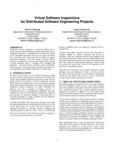
interrupt that samples the Program Counter (PC). While this method allows a precise tabulation of the number of times each function is called, the timing information it obtains from the execution is not as accurate. At specific intervals, normally every 10ms (100Hz), gprof samples the PC [27]and increments the execution time of the corresponding function by the sample time. This means that unless the total runtime of the application is significantly larger than the sampling period, the measured execution time for each function may be misrepresentative of the actual execution time. Therefore, for smaller executables, applications are run numerous times so that the profiling information accumulates for a substantial runtime. Obviously, there is a trade off between using a statistical runtime profiler and simulation to profile software execution on a processor. Statistical profilers obtain values that are imprecise and there is overhead to running the profiling software. However, the runtime profiling overhead is negligible compared with the time required to provide cycle accurate information by simulation. In other words, while gprof may add additional seconds or minutes to a software application’s execution, cycle-accurate simulation requires seconds to minutes to simulate each cycle of a hardware system, depending on its complexity. III. E MBEDDED S YSTEMS ON FPGA S When creating embedded systems, designers need to consider system requirements including performance, power, area, and cost. If a designer chooses to implement an embedded system as an FPGA SoC, it constrains some of these parameters. For example, when a designer selects a specific device, it has a set purchase price and a fixed set of resources, independent of those used by the system. We propose that by adapting the general hardware/software codesign methodology discussed in Section II to use the extra resources on-chip during the design process, designers can verify functionality and measure performance on-chip, thereby decreasing the simulation time for the system and reducing design time. A. Design Methodology Figure 1 illustrates our proposed design methodology and highlights the phases of the design process for which we have provided new design infrastructure. The process begins by describing the entire application in software, maximizing the modularity to simplify the partitioning of the application into hardware modules if it fails to meet the performance criteria. Designers can choose to verify the fully software implementation on-chip or on a personal computer, since

D. GNU’s gprof To use GNU’s gprof, the designer must compile and link the application with the profiling options enabled. Unlike PAPI, the compiler automatically generates and inserts the extra code necessary for generating the profile information used by gprof. This code counts the function calls and generates an 3

general purpose processors operate at significantly higher clock speeds than soft processors on FPGAs. However, when profiling the software’s performance, it is important that it be done on the soft processor to obtain an accurate profile. We have created a Snooping Profiler (SnoopP) that profiles performance on-chip and can be used to detect the throughput and latency of a code region/module as well as which code regions incur the greatest amount of execution time. SnoopP is discussed in detail in Section V. If the profiled performance of the system fails to meet the specified requirements, the designer partitions the application into software and hardware modules to improve performance. SnoopP’s profile information can be used to determine which software functions should be moved to hardware to speedup the application’s execution. The designer then maps these modules to the necessary processor(s) and hardware modules to create a new system platform. We propose that the designer use the SIMPPL model [4], described in Section IV, for the system architecture so that system-level interconnections can be autogenerated using our System Generator [4], as detailed in Section IV-C. Otherwise, the designer must custom-build the system’s architecture using the vendor specific system tools. After creating the new system-level architecture, the designer then implements the new hardware modules and updates the software for the new mapping. Now that the design comprises both software and hardware modules, verification can become more time consuming if a designer relies primarily on simulation to test newly designed or updated modules. However, if the designer uses the SIMPPL model for the system’s architecture, then an easily programmable on-chip testbed, outlined in Section VII, can be used to test modules orders of magnitude faster than simulation. After the system has been functionally verified, it is reprofiled to determine if it meets performance requirements. SnoopP can detect if the current platform of software and hardware modules is not processing data quickly enough for the application’s requirements. Performance degradation also arises from communication bottlenecks that force modules to stall while waiting for data to process. To complement our tool SnoopP, WOoDSTOCK is designed to monitor the fixed communication links between modules in the SIMPPL model to detect communication bottlenecks. Monitoring system communication on-chip allows designers to run the system for extended periods to detect communication bottlenecks that occur over time without having to use simulation to determine which module(s) are responsible for the bottleneck. Once the profiling data has been obtained, the designer needs to determine whether the current implementation of the system meets the specified requirements. If not, then the designer iterates through the repartitioning and redesign process, using the performance and communication profiling information to guide their decisions until the requirements are met and the design is completed. A possibility for future research is to provide this profiling information to an automated tool set that repartitions and remaps the application based on this data. However, for the purpose of this paper, we focus on highlighting the benefits of using on-chip profiling and verification tools as summarized in the following section.

B. Benefits of Designing Embedded Systems using FPGAs The premise of our design methodology is that simulating the cycle-accurate performance of a reconfigurable circuit is extremely computationally intensive and should only be used to determine preliminary functionality and not performance. Since an FPGA design platform is reconfigurable, using onchip profiling and verification tools during the design process allows designers to obtain accurate information quickly. They obtain direct feedback on the design’s actual behaviour by using the reconfigurable environment to test the system, instead of simulation, which can reduce overall design time. However, profiling on-chip not only obtains results quickly, but enables designers to profile their system using runtime data to detect data dependent behaviour. The profiler’s accuracy is determined by the operating frequency of the profiler relative to that of the rest of the system. If the operating frequency is the same as that of the system, the profiler will provide clockcycle accurate results. The designer can also run the profiler at a slower operating frequency and obtain a statistical profile, similar to gprof, if that is sufficient for the application. All of the on-chip tools are independent hardware modules that are scalable and adaptable to the system-specific architectures of different applications. Both of the profiling tools use snooping to detect the events they are measuring. They monitor signals inherent to the system so that the system’s operation is unaffected by the profiling. Neither SnoopP nor WOoDSTOCK insert extra software code into the application, which ensures that software performance is unchanged by the addition of a profiler. Furthermore, the profiling tools do not add extra hardware circuitry into the application’s processing path, ensuring that the functional operation of the system is not altered by the profiler. While the profiling tools are nonintrusive to the system’s processing, the additional circuitry may have side effects on the system’s performance by reducing the maximum clock frequency of the design depending on the percentage of the chip resources required to implement the system. In situations where the application uses the majority of the chip resources, a larger chip from the same family can be used during the design process to reduce the effects of the on-chip design tools on the maximum clock frequency. The most important benefits to designing hardware/software codesigns on an FPGA are that there is no need to finalize the partitioning of the design at the beginning of the design process or to create a complex cosimulation environment to model communication between hardware and software. The system can be run on the reconfigurable fabric where the precise interaction between hardware and software can be tested and it is easy to iterate between partitioning and profiling the design. Furthermore, the accuracy of on-chip profiling information makes it easy to provide better feedback for the partitioning process. IV. S O C M ODEL Before describing the on-chip design tools we have created for our methodology, we discuss the SIMPPL system model and the experimental platform that is currently supported by our design infrastructure. Defining a system-level architecture 4

c

off-chip on-chip

0

CE

CE

1

...

N-1 Instruction & Data Memory

CE

CE

CE

0

1

...

M-1

c

Fig. 3. CE

c

c

Fig. 2.

CE

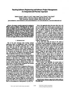
The system generator’s generic computing element.

requirements of each CE. This format of communicating data between modules is akin to software design, where the stack provides the physical interface between software functions, similar to the proposed internal links. However, the information passed on the stack, such as the number of parameters, is determined by the individual function calls. In the SIMPPL model, the size and nature of the data in the packet communicated between the IP modules performs this task. Each module has internal protocols capable of properly creating and interpreting the information in a packet.

A generic SoC described using the SIMPPL model.

and system communication protocols is essential to allowing us to autogenerate application-specific on-chip system profilers and testbenches. If there is no fixed system model, then designers would have to custom-build these design tools for every system being designed, increasing the design time and reducing the benefits of designing on-chip.

B. Experimental Platform

A. SIMPPL Model

The methodology and benefits described above are applicable to designing on both Altera and Xilinx FPGAs with either NIOS or MicroBlaze soft processors. To test our tools and demonstrate how they could be used as part of an onchip design methodology, we used the Xilinx Multimedia Board with a Virtex II 2000. All the systems and on-chip software are synthesized and compiled with Xilinx’s EDK tools. Xilinx’s MicroBlaze soft processor can be configured for application-specific requirements to improve the performance of the system. However, since the objective of this work is to study the tools for a methodology, the default parameters for the MicroBlaze core are adequate. These include a software implementation of the multiply/divide instructions and no data or instruction caches. The MicroBlaze also includes eight master and eight slave ports for asynchronous FIFOs. Xilinx has included read and write access instructions to these ports, which they call Fast Simplex Links (FSLs), so that data transfers can be implemented directly in software. To access FIFO ports directly from a NIOS processor, designers can create applicationspecific instructions that will also allow them to access the FIFOs from software. All of the on-chip tools currently use the MicroBlaze Debug Module (MDM) to upload information from the chip to the host computer, where the xmd monitor program provides the user interface. To run these tools on Altera chips requires the present I/O interface to be adapted to Avalon bus protocols.

Our proposed SIMPPL model represents SoCs as Systems Interfacing Modules with Predefined Physical Links (SIMPPL) [4], implementing an SoC as a combination of different Computing Elements (CEs) that are connected via communication links. Figure 2 illustrates a possible embedded system processing architecture described using the SIMPPL model, where the solid lines indicate internal links and the dotted lines indicate I/O communication links. I/O communication links may require different protocols to interface with off-chip hardware peripherals, but the internal links are standardized physical links with defined communication protocols to make the actual interconnection of CEs a trivial problem and to create a framework for embedded systems design. For our current work, we assume the internal links are Asynchronous FIFOs with a user defined depth. Asynchronous FIFOs simplify multi-clock domain systems, allowing designers to isolate different clock domains in different CEs and buffer the data transfers between CEs. Point-to-point links offer higher bandwidth than shared buses. Recent work also shows that commercial FPGA routing fabrics can implement network topologies where CEs have a high degree of connectivity without performance degradation due to routing congestion [28]. The SIMPPL model is comparable to Kahn [29] and Data process networks [30], except the links have finite capacity and there are no restrictions on the nature or functionality of a CE. A previously proposed model for the future of SoC design using many interacting heterogeneous processors [31] can also have this structure, however, the SIMPPL model is more general, allowing CEs to depict either processors (software CEs) or dedicated logic modules (hardware CEs). Each CE has the generic structure shown in Figure 3, where each CE has N input links and M output links. Internal links connect a CE to other CEs, where input links connect to parent CEs and output links connect to child CEs. The information passed between CEs is abstracted from the links themselves and instead, the data transfers are adapted to the specific

C. System Generator The System Generator tool generates systems of CEs comprising software and hardware CEs based on a description of the system provided by the designer. This facilitates generating example systems for testing our tools. The software CE template consists of a soft processor with its own local instruction and data memory, as shown in Figure 3, and source code that provides read and write functions to the input and output links 5

Off-chip peripheral interface

and a sample main program. The main reason for using local memory is that sharing memory creates possible data hazards. Even if two processors share a block of memory but have two distinct address spaces, there will be bus contentions causing interference in the execution results. Here, it is assumed that each of these modules should have the same performance independent of the number of other CEs in the system and that there is no need to share data between two CEs unless it is sent via a link. Each CE’s autogenerated source program file is stored on its local memory and provides functions for receiving and transmitting over the links and constants representing the processing time required to generate output data for the CE. The hardware CE template is a VHDL file that includes state machines for accessing the input and output links as well as a demonstration of how output generation can be synchronized to the availability of inputs. The generality of the System Generator provides designers with a system template that models sequential consumption and generation of data by all the system CEs. While modelling pipelining and other forms of parallelism is possible with hardware CEs, the objective is to create the physical interface and logic communication protocols so that designers can focus on CE functionality as opposed to inter-CE communication. Even though the CE templates may not exactly model a particular internal functionality, the system level communication model provides suitable benchmarks for WOoDSTOCK. Designers can also easily replace the template source code files and template VHDL functionality with their own designs. Since I/O communication links cannot be automatically generated, off-chip peripherals that produce/consume system data are modelled as part of the CE to which they are connected. If there are no internal input links (N=0) to a CE, then it generates output data by modelling input received from an off-chip hardware peripheral that must be processed before generating an output. Similarly, if a CE has no output links (M=0), all data is consumed to model output generated for an off-chip hardware peripheral. The System Generator currently creates all the necessary source files to describe a unique project for the Xilinx Platform Studios (XPS) software, however, it could easily be adapted to generate the appropriate system files for Altera’s SOPC Builder. These files are generated based on an input description file of the system provided by the user. The input file describes the number of CEs, internal links, clock domains, and external memory banks in the system. For each CE, the user details its clock domain and how it generates outputs as a function of its inputs. For software CEs, there is a final option of selecting if an external memory is included. The project file is designed to generate a download file that includes all of the executable source files for the processors. After the bitstream is downloaded onto the FPGA, all the processors start and begin running their program.

host PC

System-Level Bus

system-level bus interface

Address/ Function Decider

Soft Processor PC_EX

clock

reset clock

valid_PC

Counter 0

Counter 1

...

Counter N-1 clockcycle counters

valid_addr current_addr

S n o o p P

Counter N-1: reset clock valid_addr Address Comparators: PC=lo address

Fig. 4.

The Generic SnoopP Architecture.

SnoopP, the results are compared with those obtained using gprof. Concurrent work has also been done at the University of Ljubljana to develop a profiler for soft processors that is similar to SnoopP, called COMET [32]. COMET is demonstrated using the NIOS processor and the main goal is to use COMET as part of a hardware/software design flow to help estimate performance and guide hardware/software partitioning. A. General Architecture SnoopP is designed as an independent hardware module that the user includes in their system design. The internal structure, shown in Figure 4, subdivides into two components – the clock-cycle counters and the system bus interface. The former profiles the system with the user-specified number of counters while the latter provides off-chip access to their values. To profile source code execution, SnoopP connects to a bus that displays the executing Program Counter (PC EX) bus and a valid instr signal that is high when the value on the PC EX bus is valid. Each code segment counter increments every time the value of the PC EX bus is both valid and in range. When designers clock SnoopP using the system-level clock, as shown in Figure 4, this results in an accurate clockcycle count of the time spent in a code segment. To obtain a cycle-accurate profile of data region accesses, instead of source code execution, SnoopP’s counter address bus needs to be connected to the system address bus and a “valid data address” signal. It should also be noted that SnoopP can be used to obtain a statistical profile of data accesses or program execution, similar to gprof. Using an independent clock to drive the module, instead of the system-level clock, allows the user to choose an appropriate clock frequency that provides them with an adequate granularity for their profiling data. Counter N-1 is magnified to illustrate the internal workings of a clock-cycle counter. To determine if the address, for example the PC EX, is in range, comparators check to see if the present PC EX value is between the specified low and

V. S NOOP P This section describes the architecture and experimental evaluation of our on-chip software profiler called SnoopP. To demonstrate the accuracy of profiling an application with 6

high addresses. If the PC is valid and is presently accessing an address within these bounds, then the counter value is incremented. The counters are memory mapped to the system-level bus, which enables a user to read and reset the counters from a host computer via the off-chip interface module connected to the system-level bus. Thus, SnoopP allows the designer to measure the exact number of clock cycles the program spends executing specified code segments or accessing data memory at runtime.

While this architecture provides the user with significant flexibility for profiling software, the hardware required to implement SnoopP with the maximum 16 counters translates into a maximum circuit size that utilizes 849 flipflops and 1349 LUTs for logic. The 16 46-bit counters require 736 flipflops, accounting for 87% of the flipflops utilized by SnoopP. Alternatively, SnoopP’s counters could also be implemented using an on-chip Block RAM (BRAM), however, this would reduce the flexibility of the code segment definitions. The user would have to constrain their definition such that no more than two code segments overlap for a given address. This limitation arises because the BRAMs allow up to two concurrent memory accesses. The remaining 13% of the flipflops in SnoopP latch internal control signals to prevent the system’s critical path from being in SnoopP when the system is synthesized. For simple soft processor systems, SnoopP does not limit the maximum clock speed and, ideally, the profiling circuit will never be on the system’s critical path as its maximum operating frequency is 127MHz. However, if the design is approaching the capacity of the FPGA, it may be unavoidable. If necessary, SnoopP can be pipelined to reduce the delay path in faster systems. This includes latching the current address and system ABus buses and the valid addr and system ABus select signals. These additions have not been incorporated into the present version of SnoopP as they are unnecessary and increase the size of the circuit. To implement the 32 32-bit comparators used to determine if an address is within each counter’s address range requires 1024 LUTs. This encompasses 76% of the LUTs employed in the SnoopP, and does not include the logic required to interface SnoopP to the OPB. The OPB interface must use two comparators to resolve that the user has accessed the SnoopP memory space. More logic is required to select the counter operation and to implement a 16-to-1 multiplexer that drives the appropriate value onto the OPB. Thus, the resources necessary to implement SnoopP using 16 counters is actually larger than what is required to implement a MicroBlaze processor, and an area for future study is possible methods of minimizing the size of SnoopP, such as reducing the resolution of the comparators for the address ranges.

B. Design Decisions SnoopP allows the user to choose up to a maximum of 16 profiling counters to limit the circuit size. Each counter requires two comparators to determine if the 32-bit address is in a valid range. The user can obtain the addresses for the upper and lower bound parameters of the address ranges by assembling the code or reading the symbol table. To provide complete flexibility in specifying the address ranges, SnoopP allows designers to select address ranges as small as a specific address to an entire 32-bit address space. This means that when SnoopP profiles source code, a code segment could be anywhere from a single instruction to an entire program. Currently, designers must select the number of counters, their individual address ranges, and their location in the memory map pre-synthesis to limit the effects of parameterization on SnoopP’s critical path delay. Since it is desirable to be able to reload the address boundaries between application runs, the designer can easily change SnoopP to support runtime programmable address ranges if clock speed is not a concern. However, a better option would be to enable the designer to update the bitstream to change the hardwired address ranges without re-synthesizing the design. Currently, there are some tools that could be used by designers to do this, but there is no clear, user-friendly tool flow that provides easy access for making these changes. However, such a tool is feasible to implement for future work. When using SnoopP, it is important to remember that only address accesses in contiguous regions of memory are counted. For example, to accurately profile how long a function A with subfunction calls X, Y, and Z takes to execute, the user must assign a counter to the function as well as to each of the subfunctions called during its execution (i.e. A, X, Y, and Z). Furthermore, if another function B calls any of these subfunctions, for instance Y, it may not be possible to distinguish which portion of the subfunction Y’s execution time is due to function A versus function B. Since most software programs require many cycles for completion, 46-bit counters are used to store the clock cycle counts, which is equivalent to letting the profiler run at 100 MHz for eight days. When profiling source code, the decision to count clock cycles, as opposed to the number of executed instructions, is based on the desire to be precise as to the actual time spent executing each code segment. Given that most code segments will include a branch and/or a memory fetch, there will likely be pipeline stalls that could significantly increase the time spent executing a segment. This stall time is not accounted for if only the number of executed instructions are counted.

C. Experimental Evaluation This section illustrates how SnoopP profiles source code using Dhrystone [33] as a sample benchmark. It details the methodology used and the issues encountered when profiling the application. 1) Methodology: There are two possible methods of using SnoopP to profile software performance. The first is to use gprof to obtain an initial profile of executable performance. This information can be used to try and assign the counters to what gprof determines are the important regions of the executable. The other method is to perform all the profiling using SnoopP. To do this, the user divides the software executable into groups of functions forming continuous address blocks and obtains an initial profile. The regions that require the largest percentage of execution time can be subdivided further to determine which specific functions take the most 7

TABLE I

TABLE II

S TATISTICS ON F UNCTIONS COMPRISING THE D HRYSTONE B ENCHMARK AFTER O NE H UNDRED AND O NE M ILLION PASSES .

D HRYSTONE S NOOP P C OUNTER A SSIGNMENTS .

GPROF

Function Name internal mcount main Proc 8 Func 1 Proc 7 Func 2 Proc 1 Proc 6 Proc 2 Func 3 mcount Proc 3 Proc 4 Proc 5

100 Passes Total Calls — 1 100 300 300 100 100 100 100 100 — 100 100 100

One Million Passes Total Percent Calls Time — 1 1000000 3000000 3000000 1000000 1000000 1000000 1000000 1000000 — 1000000 1000000 1000000

31.5 11.2 10.4 9.6 6.1 6.1 5.9 4.5 3.7 3.5 3.2 1.9 1.6 0.8

Counter Number

Function Name

Number of Instructions

Percentage of Static Code Size

0 1 2 3 4 5 6 7 8 9 A B C D E F

main Proc 1 Proc 2 Proc 3 Proc 4 Proc 5 Proc 6 Proc 7 Proc 8 Func 1 Func 2 Func 3 divsi3 malloc mulsi3 strcmp

376 70 16 18 24 7 42 5 60 11 49 9 38 11 22 32

43.5% 8.1% 1.9% 2.1% 2.8% 0.8% 4.9% 0.6% 6.9% 1.3% 5.7% 1.0% 4.4% 1.3% 2.5% 3.7%

TABLE III C YCLE -A CCURATE R ESULTS USING S NOOP P TO P ROFILE D HRYSTONE ON

execution time. Depending on the size of these regions, the number of functions and the division of execution time, the user may have to iterate through this process until a suitable performance profile has been obtained. For the purpose of this study, we used gprof to provide a baseline comparison of the varied accuracy between statistical and clock cycle accurate profilers. The application is initially profiled with gprof on a Sun Ultra 80 Model 4450 running version 5.8 of the Solaris OS. The design is then run on a MicroBlaze processor instantiated on the FPGA and profiled with SnoopP for more precise performance information. The application is compiled using gcc -O2 for both the Sun and MicroBlaze platforms, which optimizes the application’s source code without inlining functions. Finally, we use Xilinx’s version of gprof tailored to run on the MicroBlaze, mbgprof and profile the application on running on three different configurations of the Microblaze. We can then compare the results to determine if using mb-gprof on the MicroBlaze obtains profiling data that correlates better to the SnoopP profile than using gprof on the Sun station. 2) Dhrystone: Dhrystone is a synthetic benchmark for testing a system’s integer performance that Xilinx uses to measure MicroBlaze processor performance. Table I summarizes the results obtained using gprof on the Sun workstation. Column 1 contains the function names for which gprof returns results. Columns 2 and 3 list the number of times each function is called when Dhrystone makes one hundred passes and one million passes through the main loop respectively. Finally, Column 4 reports the percentage of execution time that gprof attributes to each function when the main loop makes a million passes. gprof is unable to obtain the same type of statistical timing information when Dhrystone makes only one hundred passes of the main loop as it completes execution in less than 10ms on the workstation. The functions internal mcount and mcount are part of the profiler and count the number of times a function is called during execution. While gprof does not report the number of times these functions are called, their

M ICRO B LAZE SYSTEMS THAT INCLUDE AND EXCLUDE THE H ARDWARE M ULTIPLIER AND D IVIDER . Function Name

Percentage of Execution Time (100 Passes)

Percentage of Execution Time (A Million Passes)

Percentage of Execution Time (100 Passes) HW multiply

Percentage of Execution Time (100 Passes) HW multiply & divide

mulsi3 divsi3 main strcmp Proc 1 Proc 8 Func 2 Proc 6 Proc 3 Func 1 Proc 4 Proc 7 Proc 2 Func 3 Proc 5 malloc

23.49 14.88 14.75 10.80 9.62 7.49 4.88 3.39 2.17 1.98 1.75 1.64 1.54 0.82 0.76 0.02

23.56 14.93 14.51 10.83 9.65 7.52 4.89 3.40 2.17 1.98 1.76 1.65 1.54 0.83 0.77 0.00

— 20.68 19.22 15.00 13.37 5.39 6.78 4.72 3.01 2.75 2.44 2.28 2.13 1.15 1.06 0.03

— — 23.90 18.99 16.92 6.83 8.58 5.97 3.81 3.48 3.08 2.89 2.70 1.45 1.34 0.04

combined overhead accounts for 34.7% of the execution time calculated by gprof. Since this application only has a few functions, it is possible to assign the counters in SnoopP to almost every function, profiling 91.5% of the static code size. Only the initialization and clean up portions of the executable are ignored as they add little overhead and cannot be moved to hardware. Table II outlines how the application is partitioned into profiling segments. It includes the number of instructions per code segment and the percentage of the static code size utilized by each function to give better context to the profiling results. Table III contains the results obtained from profiling the 8

Dhrystone benchmark on the FPGA using SnoopP. The percentages assume that the total execution time can be approximated by summing the time spent executing the functions within the user written portion of the executable. The results in Columns 2 and 3 are run on a MicroBlaze processor that implement integer multiplies and divides using software functions and run the main loop for one hundred and one million passes respectively. Columns 4 and 5 assume that the main loop runs one hundred passes, but varies the MicroBlaze platform to include a hardware multiplier and then to include a hardware multiplier and divider. By comparing the percentage execution time results in Tables I and III, we see that there is a significant difference between results obtained by SnoopP versus gprof. Not only are the execution time percentages different, but gprof ranks Proc 8, Func 1, and Proc 7 as the top three of the application’s functions consuming processing time. In contrast, SnoopP shows that the application functions Proc 1, Proc 8, and Func 2 actually consume the most processing time on a MicroBlaze. Furthermore, the software implementations of the integer multiply and integer divide functions along with main require just over 53% of the processing time. Therefore, if the partitioning choices are based on the profiling results obtained from gprof, the designer would not select the appropriate functions to implement in hardware. Comparing Columns 2 and 3 illustrates the consistency of profiling information obtained using SnoopP. While gprof is only able to obtain a timing profile by executing the Dhrystone main loop a million times versus one hundred times, SnoopP obtained results that vary by no more than 0.24% for both cases. The resulting variance is easily explained by the diminishing significance of initialization code within main with respect to the longer execution time of the main processing loop. Therefore, SnoopP is able to obtain more accurate and consistent results than gprof in only 0.01% of the execution time. Column 4 illustrates how the removal of the software multiply instruction increases the percentage execution time of all of the functions except for Proc 8. This exception occurs because the number of instructions in the Proc 8 function dropped from 60 to 33 due to optimizations that were possible with the removal of the software multiply. The inclusion of a hardware multiplier reduced the execution time of the application from 1.33 million clock cycles to 960 thousand clock cycles, approximately 28%. The extra resources required to implement the multiplier were 39 LUTs, 50 FlipFlops, and three 18x18 dedicated multipliers. Given the significant improvement in performance obtained using these minimal hardware resources to implement the hardware multiplier, we decided to investigate the benefits of including the hardware divider in combination with the multiplier. The additional resources required to implement the hardware divider are 117 LUTs and 109 FlipFlops, but it further reduces the execution time by another 15%. Depending on the requirements of the application, the designer may feel that this is an acceptable tradeoff. Next mb-gprof was used to profile Dhrystone using the same three configurations of the MicroBlaze profiled by SnoopP.

We profiled Dhrystone running for both 100 and one million passes and also set the mb-gprof parameters to mimic those used in gprof on the Sun station. However, the clock frequency of the Sun station’s processor is 450MHz, whereas, the MicroBlaze processor is running at 27 MHz. Therefore, the Sun station’s processor executes 16.7 times the number of clock cycles as the MicroBlaze during the same period. Table IV summarizes the results of profiling Dhrystone using mb-gprof. Column 1 lists the function names for which mb-gprof returns profiling results and the remaining columns report the profiling data for the different experimental set ups. Dashes are used in these columns to indicate when mbgprof returned no data on the percentage of execution time. The results in Columns 2 and 3 are run on a MicroBlaze processor that implement integer multiplies and divides using software functions and run the main loop for one hundred and one million passes respectively. When Dhrystone executes 100 passes mb-gprof is only able to sample the PC eleven times at runtime, thus the remaining configurations have Dhrystone run for one million passes Columns 4 and 5 varies the MicroBlaze platform to include a hardware multiplier and then to include a hardware multiplier and divider respectively. Since mb-gprof is run on the MicroBlaze, it is able to profile the software implementations of the multiply and divide functions. Columns 2 and 3 illustrate that mb-gprof detected the software multiply as the second largest consumer of execution time, as opposed to the top consumer as indicated by SnoopP in Table III. Columns 4 and 5 show Func 1 and Proc 7 as two of the top three consumers of execution time similar to gprof (see Table I). These results demonstrate that even though the PC is sampled 16.7 times more by mb-gprof than by gprof on the Sun station, statistical profiling still creates a highly inaccurate profile compared to SnoopP. In summary, SnoopP produces a fast, consistent, clock cycle accurate profile of of a systems’s execution performance as demonstrated with the Dhrystone example. While, gprof is able to obtain a basic overview of software performance, it needs numerous more loops of the main algorithm to obtain its percentage of execution time per function. Moreover, this data is obtained on a distinctive instruction set architecture (ISA) from the MicroBlaze using a statistical profiler. Its results do not match the exact results measured by SnoopP. However, an initial profile from gprof can facilitate the assignment of the SnoopP counters to the appropriate code segments as it indicates which code segments likely require the most execution time. mb-gprof may be able to provide slightly better profiling data than running gprof on the Sun station since it uses the MicroBlaze ISA. However, the time required to profile an application using SnoopP is less than time required for mb-gprof because of the additional software profiling functions added to the executable at compilation time for obtaining profiling data. Therefore, there is greater value in using SnoopP to obtain clock-cycle accurate results rather than the statistical results acquired using mb-gprof. VI. WO O DSTOCK When creating embedded systems, designers need not only consider the independent performance of each module in the 9

TABLE IV running

MB - GPROF S TATISTICS ON

F UNCTIONS COMPRISING THE D HRYSTONE B ENCHMARK AFTER O NE H UNDRED AND O NE M ILLION PASSES .

Function Name

start1 mulsi3 Func 2 Proc 1 Proc 3 Proc 5 Proc 8 main strcmp Func 1 Proc 7 Func 3 Proc 2 Proc 4 Proc 6 divsi3

Percentage of Execution Time (100 Passes)

25.00 16.67 8.33 8.33 8.33 8.33 8.33 8.33 8.33 0.00 0.00 0.00 0.00 0.00 0.00 —

Percentage of Execution Time (A Million Passes)

0.00 10.20 5.38 7.17 4.55 3.73 8.97 8.55 5.52 10.07 10.21 3.59 4.55 4.55 5.66 7.31

Percentage of Execution Time (A Million Passes) HW Multiply

Percentage of Execution Time (A Million Passes) HW Multiply & Divide

— — 0.00 9.09 5.79 0.00 9.09 0.00 9.09 18.18 12.40 9.09 9.09 9.09 0.01 9.09

0.00 — 6.50 13.63 4.55 5.19 7.47 10.72 7.79 13.31 12.34 5.19 5.19 2.92 5.20 —

running

M1

running

M3

CE3

CE1

M0

CE2

M2

running

Monitor Controller cntr_address valid_cnt

CE0

running

system-level bus host PC

Fig. 5.

Off-chip peripheral interface

The WOoDSTOCK architecture.

2 FIFO_1 full

unknown

1

1

FIFO_0 not full

FIFO_0 empty

0

0

(a)

(b)

FIFO_0 full

1 unknown

(c)

Fig. 6. Examples of the different types of bottlenecks detectable by WOoDSTOCK: (a) interior bottleneck, (b) input bottleneck, and (c) output bottleneck.

design, but they must also ensure that there is load balancing among the CEs. If not, system stalls may be the reason a design fails to meet performance requirements. This section describes how Watching Over Data STreaming On Computing element linKs (WOoDSTOCK) can be used to monitor system behaviour.

hardware that records the behaviour of the traffic on all the internal input and output links connected to its CE through internal counters. These counters are used to measure the total possible stalling/starving time for a CE during the profiling period, which is set based on the program execution of a specially selected base processor, labeled as CE0 in Figure 5, or an independent execution time counter. The user sets the active monitoring period of the system based on the region of a base processor’s source code or an independent execution time counter. Addresses of the instructions bounding the code region or the minimum and maximum counter values are provided to WOoDSTOCK as start and stop points. The running signal, shown in Figure 5, is enabled and disabled when the start and stop values, respectively, are seen as valid values on the counter bus. This signal is used to enable or disable the system’s monitors. Each of the CEs and their monitors in Figure 5 are labelled for the purpose of differentiating the base processor (CE0) from the remaining CEs (1,2,3).

A. Multi-CE Profiling Architecture The SIMPPL model described in Section IV-A resembles a multiprocessor system, where software designers are able to obtain some run-time statistics about an application’s behaviour on their system. Of particular interest is the ability to determine the stall time of individual processors in the system. Typically, a scheduler monitors when a processor is waiting for another processing task, but as the scheduler is unaware of the nature of the actual tasks, it only provides system-level information. WOoDSTOCK is able to provide analogous information to designers due to the standardized interface used in the SIMPPL model. WOoDSTOCK highlights problems arising from inter-CE communication and indicates to the user when a particular CE creates a system bottleneck. Like the scheduler, WOoDSTOCK is similarly unaware of the actual computation performed on a CE. Therefore, the precise cause of a system bottleneck is determined using a combination of the system performance results along with user’s knowledge of the design and independent CE profiling. In the case where a software CE is causing the bottleneck, SnoopP may be used to detect the source of the bottleneck. Figure 5 illustrates the connections between WOoDSTOCK and a multi-CE system. Each diamond represents a monitor that is associated with a specific CE. A monitor is a piece of

B. Bottleneck Detection WOoDSTOCK assumes that the only signals a monitor can connect to are the full and empty status signals of the asynchronous FIFOs implementing the internal input and output links of its respective CE. These signals are used to generate enable signals for the counters used to profile the system. The counters are used to measure the number of clock cycles where a CE is potentially starving or stalling the system. A more naive approach would be to assign individual counters to the full and empty signals of each link in the system. However, this provides less useful information to the designer as the relationship between these status signals is required to 10

TABLE V CE J-1

...

fsl_K-1_full

MEM 0

FSLs fsl_K-1_exists

determine if a CE is a system bottleneck as shown in the following paragraph. Figure 6 illustrates examples of the three types of system bottlenecks that WOoDSTOCK can be used to detect. Figure 6(a) shows an interior bottleneck, where CE 1 has both internal input and output links and is stalling the system. To understand how WOoDSTOCK determines there is a bottleneck, consider when FIFO 1 becomes full. CE 1 may not be consuming the data produced by CE 2 fast enough. However, CE 1 may also be stalled because it cannot write to FIFO 0 if it too is full, in which case a child CE is the bottleneck and not CE 1. To differentiate between these situations, a CE is defined to be an interior bottleneck when all the input links that provide data to generate a specific output are full and the link at the output is not full as depicted in Figure 6(a). The specification of the output link as “not full”, as opposed to empty, delineates an important aspect of the system monitoring tool. WOoDSTOCK is unaware of the nature of the data being transferred between CEs, so if CE 1 produces a data packet that CE 0 requires in its entirety to continue processing, then the link should normally be empty when the system is balanced. However, if CE 1 produces a data packet that is consumed as multiple individual data packets by CE 0, then there will normally be data in this FIFO even when the system is balanced. Therefore, the output link must be only “not full” instead of “empty” to produce a bottleneck. A CE that has internal output links and no internal input links may cause an input bottleneck. This occurs when either the off-chip hardware peripheral supplying input to the CE is too slow or the processing time of the CE is too slow. In either case, the system is starved for data. To detect this situation, WOoDSTOCK monitors the empty status signal of the output link. Figure 6(b) shows CE 1 as the potential cause of an input bottleneck. The status of the I/O communication link is unknown and FIFO 0 is empty. However, CE 1 may not be a bottleneck if CE 0 consumes data at the same rate as CE 1 produces it. This situation would also cause FIFO 0 to be empty for the majority of the system’s run-time. Since the results from these measurements are not conclusive on their own, the designer needs to see how this information fits in with the results obtained from monitoring the rest of the system. Output bottlenecks arise in CEs that have internal input links and no internal output links. They occur due to the slow processing rate of either the CE or an off-chip peripheral. Both cases result in the input links to the CE becoming full as illustrated in Figure 6(c). While the state of the I/O communication links is unknown, FIFO 0 becomes full stalling the system. In situations where a CE stalls or starves because of an off-chip peripheral’s slow data rate, this is

CE 0 (base uproc)

FSL Network

FSLs

fsl_1_full

MDM

CE 1

fsl_1_exists

host PC

fsl_0_full

FIFO 1 full and (not FIFO 0 full) FIFO 0 empty FIFO 0 full

fsl_0_exists

Output Equation

Interior Bottleneck Input Bottleneck Output Bottleneck

On-Chip Peripheral Bus

Bottleneck Example

FSLs

...

E XAMPLE OUTPUT EQUATIONS FOR THE SYSTEMS IN F IGURE 6.

WOoDSTOCK

Fig. 7.

The interface of WOoDSTOCK with a multi-CE system.

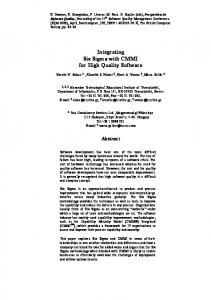
still measured as being caused by the CE implementation. Therefore, the user must be sufficiently familiar with the CE’s processing to determine the precise cause of the bottleneck. To generate a system-specific monitoring system, the user writes a description of the system that states the required combination of data on internal input links used to produce an output for a given output link. WOoDSTOCK uses this information to create an output equation for each CE output described in terms of link empty and full status signals. Table V shows the appropriate output equations for CE 1 in each of the systems in Figure 6. These equations generate counter specific enable signals that are combined with the running signal to enable all the appropriate counters during each sampling clock cycle. The frequency of WOoDSTOCK’s sampling clock can be set to any rate, depending on the desired profiling accuracy. If sampling is done using the fastest system clock, then the measured results are precise. However, a slower clock may be used to do the sampling and obtain a statistical measurement of system performance. This information can still help detect system bottlenecks, but the system may need to be profiled for longer run-times to observe the problem. C. Implementation and Design Decisions WOoDSTOCK generates the necessary system dependent VHDL files to implement the monitoring system, along with the files required by XPS to interface WOoDSTOCK into a MicroBlaze system as shown in Figure 7. The internal structure of WOoDSTOCK is subdivided into two components — the system monitors and the OPB interface. The former profiles the system links based on the user-provided system profile (recall Figure 5) while the latter provides off-chip access to their counter values. Similar to SnoopP, WOoDSTOCK is memory mapped to the OPB as a slave device and uses 46-bit counters. It also uses the MDM module as an off-chip interface to the xmd control window running on a host computer allowing users to remotely read and reset the counters. While WOoDSTOCK does not differentiate between monitoring hardware and software and CEs, the MDM module requires that there be at least one MicroBlaze processor in the 11

3 fsl_0 1

2 fsl_3

fsl_1

fsl_2 0

4

Fig. 8. An application architecture with branching using the SIMPPL model.

system. However, embedded systems are typically comprised of a combination of hardware and software, which means there should be at least one processor in the system to fulfill the MDM’s requirements. WOoDSTOCK also connects to the FIFO status signals that indicate when there is data in the FSL to read and when the FSL is full. For the purpose of this paper, these signals will be referred to as fsl empty and fsl full respectively. By monitoring their runtime values, WOoDSTOCK enables the appropriate counters based on the user-defined output equations. D. Case Study This section demonstrates how the information WOoDSTOCK provides can help to refine a design using a case study. It details the issues encountered while profiling a system and concludes with a discussion of the advantages of on-chip system profiling. 1) Methodology: The branching system architecture illustrated in Figure 8 is used as a case to demonstrate the functionality of WOoDSTOCK. We use the System Generator described in Section IV-C to generate benchmarks. The CEs in these benchmarks are implemented using the default version of the MicroBlaze soft processor. Each MicroBlaze has eight built-in FSL (FIFO) receive and transmit ports and the send and receive functions are generated based on macros provided by Xilinx to read and write from these ports. The time required for a CE to process input data to produce output data is modelled using the delay parameter in the main loop of the generated source code template. The source code for each MicroBlaze is then compiled and stored in its local onchip memories and accessed via Local Memory Buses. Each system configuration is profiled for varying lengths of time to determine the initial effects of system start up on the results. The main processing loop of the base processor uses a for loop to set the number of data packets it consumes. Therefore, we can vary the profiling period is by changing the upperbound of the for loop. The branching system architecture is used to highlight the increasing difficulties of analyzing systems that are less intuitive than pipelines. WOoDSTOCK uses the global system clock as its sampling clock and the different configurations of the system are created by varying the delays used to model CE processing times. These processing delays are used to create system imbalances that WOoDSTOCK should report as well as balanced systems to determine how this affects the results obtained by WOoDSTOCK. 2) Branching System Example: Figure 8(b)’s branching system requires 8 counters that are enabled based on the 12

functions described in column 2 of Table VI when the monitors are running. Counters 0 and 1 monitor fsl 1 and fsl 2 to determine if CE 0 is stalling the system. Similarly, counters 2 and 6 measure when CE 1 and CE 4, respectively, stall the system. Counters 3 and 4 count the number of clock cycles for which fsl 2 and fsl 3 are empty as does counter 5 for fsl 0. This information can help to determine if either CE 2 or CE 3 are producing output data too slowly, and thus starving their respective children CEs. The possible interpretations for the counter values are summarized in column 3. In this system, each data packet to and from each link is processed independently. For example, in CE 2 an output is generated for fsl 2 after a processing delay and an output is generated for fsl 3 after a separate processing delay. Therefore, for CE 2, the time between generating outputs for fsl 2 is the sum of these two delays. Similarly, in CE 0, data is read from fsl 1 followed by a processing delay before data is read from fsl 2 followed by an independent processing delay. In this case, for CE 0, the time between reading inputs from fsl 1 is the sum of these two delays. The first configuration of this system has all of the processing delays for each link set to the same value. This creates an imbalanced system as CE 0 and CE 2 have an effective per link processing delay that is twice that of the other CEs. Again, the base processor’s for loop is set to consume 20, 100, and 200 data packets, which is sufficient to demonstrate the system imbalances for the following configurations. Table VI summarizes the results for Configuration A in the subcolumns labelled Con A where all values are in terms of the percentage of the monitor’s run-time for which the counter was enabled. The total profiling period is reported to the nearest million clock cycles in Counter 7’s row. The importance of running the system for a significant period of time is highlighted by the results for counter 0, which vary from 21.4% to 91.8%. The larger value from the long runtime clearly indicates that CE 0 is stalling the system by not consuming data quickly enough. To try and remove this bottleneck, CE 0’s processing delays for input data read from fsl 1 and fsl 2 are reduced to 50% of the delays for the rest of the system. This means that the combined effective per link processing delays for fsl 1 and fsl 2 are now the same as the rest of the system, with the exception of CE 2’s processing delays, which are left unchanged. The results for this configuration are found in Table VI in the subcolumns labelled Con B. From these results, it appears that CE 0 is still stalling the system, however closer inspection disproves this theory. While fsl 1 is still becoming blocked as the run-time increases, the period for which fsl 2 is empty has increased dramatically (see Counter 3). This may indicate that CE 2 cannot keep up with its child nodes. If this is the case, CE 0 is now starved for data on fsl 2 and still not able to keep up with its parent node CE 1. This also is reflected in the overall run-time that remains basically unchanged between Configuration A and Configuration B as the profiling period increases. If CE 0 were the only bottleneck in the system, the system’s performance should have increased noticeably. Therefore, CE 2 must also be a system bottleneck, failing to provide data at the necessary production rate.

TABLE VI TABLE FOR BRANCHING SYSTEM COUNTER RESULTS DESCRIBING THE COUNTER ENABLES , WHAT THE COUNTERS REPRESENT, AND REPORTING THE MEASURED RESULTS AS PERCENTAGES OF THE TOTAL MONITOR RUN TIME GIVEN IN C OUNTER 7 TO THE NEAREST MILLION CLOCK CYCLES . Cntr

Enable Condition

Possible Meaning CE 0 slow CE 0 slow CE 1 slow

21.4 0 0

10.1 0 0

0 0 0

83.7 0 0.0

82.2 0 0.0

0 0 0

91.8 0 0.0

91.1 0 0.0

0 0 0

3 4 5 6

fsl 1 full fsl 2 full fsl 0 full and (not fsl 1 full) fsl 2 empty fsl 3 empty fsl 0 empty fsl 3 full

CE 2 slow? CE 2 slow? CE 3 slow? CE 4 slow

2.4 100.0 83.3 0

94.9 100.0 94.9 0

2.3 100.0 100.0 0

0.50 100.0 17.3 0

99.0 100.0 18.8 0

0.5 100.0 100.0 0

0.2 100.0 8.7 0

100.0 100.0 9.4 0

0.2 100.0 100.0 0

7

running

monitors on

672

632

352

3232

3192

1632

6432

6392

3232

0 1 2

System under Test (SUT) Source uproc

Fig. 9.

CE

CE . . .

Source & Sink uproc

20 Data Packets Con A Con B Con C

200 Data Packets Con A Con B Con C

tion protocols of a CE allow the designer to use a flexible testbed architecture as shown in Figure 9. CEs can be verified individually, as independent processing stages, or in combination with adjacent CEs. Furthermore, since the design is implemented on an FPGA, it is possible to run the testbed on-chip to verify the behaviour of CEs‘ with a large number of data packets to obtain quick and accurate results. Previous work demonstrated that debugging [34], [1] and profiling [4] designs using on-chip resources results in a significant reduction of the time required to obtain information for the designer. Since design verification commonly requires greater than 50% of the overall design time, sometimes as much as 70% [35], it may be possible to reduce the percentage of time spent verifying the design, and thus reduce the overall design time.

SUT CE

100 Data Packets Con A Con B Con C

Sink uproc

The on-chip testbed for debugging CEs.

By reducing CE 2’s processing delay for generating outputs for fsl 2 and fsl 3 to 50% of the original processing delay, the system should be balanced. This is designated as Configuration C and the results are found in the subcolumns labelled Con C in Table VI. In this case, none of the links become full so the system never stalls. This produces the expected increase in the overall system performance by decreasing the overall run-time by approximately 50% from the Configuration A. 3) Summary: WOoDSTOCK is able to detect bottlenecks in system performance and the removal of these bottlenecks dramatically improves the overall performance as demonstrated in the above examples. WOoDSTOCK required 928 LUTs and 478 flipflops to monitor the branching example. If these results are normalized in terms of the number of counters in each system, the branching example uses 116 LUTs and 59.8 flipflops per counter. These results highlight that the increased size of WOoDSTOCK is mainly due to the extra counters and that overhead logic needed to provide a user interface can be considered minimal. The system must be run for a significant period of time to obtain accurate results using WOoDSTOCK. This may be on the order of minutes to hours depending on system complexity, and is necessary to account for the initial effects of starting up the system. If these results are to be found via simulation, the required time could be excessive. Although WOoDSTOCK obtains only a macroscopic view of system performance, combined with an understanding of the individual CEs, it provides greater insight into system behaviour that can guide the redesign of a system. Finally, while a designer should be sure that there are no CEs stalling the system, interpreting the meaning of the measured results for more complex systems requires that the Counter values not be viewed in isolation as demonstrated by this example.

The testbed comprises the processors and the software required to generate (Source) and interpret (Sink) data packet streams for the CEs. The MPEG-1 video decoder is designed for a Xilinx Virtex2V2000, so the MicroBlaze T M soft processor is used in this testbed. High-level functions are built to generate each data packet from the instruction and data pointer specified by the user. The user can then quickly alter the number and types of data packets sent by the Source to the System Under Test (SUT) by changing the instructions in the source code and then compiling and downloading the processor executable to the Source Processor. Creating the data stream using software allows a significantly quicker turnaround time for testing the SUT with different data packet streams than is possible with the source data stream coded as a separate hardware module. The Sink Processor runs a program that detects and interprets packets received from the SUT and then allows the user to log them. The Sink processor program can also be combined with the Source processor program to allow designers to log the intermediate state of the design as shown in Figure 9. The on-chip testbed facilitated the detection of a significant PE error that required the redesign of the MPEG-1 video decoder pipeline. Using the MPEG-1 pipeline from the VLD/RLD CE to the MC/PR CE as the SUT, the design team found that a portion of the design specification for the MC/PR PE had not been implemented. The team created a new CE called the Missing Macroblock Replacer (MMR) CE and inserted it into the decoder pipeline just before the MC/PR CE

VII. O N -C HIP T ESTBED Our final contribution to an on-chip design infrastructure is an on-chip testbed for systems designed using the SIMPPL model. The standardized physical interface and communica13

to correct the error. The modularity and structure of SIMPPL made this change to the pipeline very easy. Although the on-chip testbed runs orders of magnitude faster than in simulation, it does not likely exhibit the exact runtime behaviour of the final system. A runtime data stream could be irregular with data words sometimes arriving every clock cycle and sometimes delayed for numerous clock cycles, thus the Source and Sink may process data slower or faster than the system at runtime. However, the Consumer and Producer controllers, which interface the CE with its preceding and subsequent CEs, are able to abstract runtime data behaviour from the PE as they separate the communication protocols from the actual data processing. Both are able to properly stall the PE if there is no source data in the Rx Communication Link or no space in the Tx Communication Link so that the PE exhibits correct runtime behaviour independent of the data rate. VIII. C ONCLUSIONS AND F UTURE W ORK In this paper, we have described a hardware/software codesign methodology tailored to FPGAs. Since the FPGA fabric is easily reprogrammed, it allows a design methodology that incorporates on-chip design tools. The benefits accrued from such an approach are similar to those experienced by software designers who typically design on a processor-based platform as opposed to a processor simulator. Designers can obtain accurate results quickly using tools that are tailored to their specific design. Moreover, running a design on an FPGA is orders of magnitude faster than simulating it, allowing a larger number of test vectors to be used to verify functionality. To support this design methodology, we have begun developing an on-chip design infrastructure. Thus far, we have created an on-chip testbed, two on-chip profiling tools, and a system-level specification tool to facilitate system-level integration. While the on-chip profiling tools are modular and scalable to system requirements, the on-chip testbed currently uses soft processors to provide the test vectors and store the resulting outputs. We have demonstrated that on-chip profiling tools quickly obtain accurate results that can be used by the designer to make better design decisions to reduce design time. The next phase of this work will be to automate this process by creating tools that incorporate the on-chip profiling results to generate a new partitioning, mapping, and scheduling for the application on a newly generated system architecture. R EFERENCES [1] K. S. Hemmert, J. L. Tripp, B. Hutchings, and P. A. Jackson. Source Level Debugger for the Sea Cucumber Synthesizing Compiler. In IEEE Symp. on FCCM, pages 228–237, April 2003. [2] R. Hough, P. Jones, S. Friedman, R. Chamberlain, J. Fritts, J. Lockwood, and R. Cytron. Cycle-Accurate Microarchitecture Performance Evaluation. In Proc. of W’shp on Introspective Arch., February 2006. [3] L. Shannon and P. Chow. Using Reconfigurability to Achieve RealTime Profiling for Hardware/Software Codesign. In ACM Int. Symp. on FPGAs, pages 190–199, February 2004. [4] L. Shannon and P. Chow. Maximizing System Performance: Using Reconfigurability to Monitor System Communications. In IEEE Int. Conf. on FPT, pages 231–238, December 2004. [5] L. Shannon, B. Fort, S. Parikh, A. Patel, M. Saldana, and P. Chow. A System Design Methodology for Reducing System Integration Time and Facilitating Modular Design Verification. In IEEE Int. Conf. on FPL, August 2006.

14

[6] S. Kimura, Y. Itou, and M. Hirao. A Hardware/Software Codesign Method for a General Purpose Reconfigurable Co-Processor. In 5th Int. W’shp on Hardware/Software Co-Design, March 1997. [7] J. Fleischmann, K. Buchenrieder, and R. Kress. Codesign of Embedded Systems Based on Java and Reconfigurable Hardware Components. In DATE, March 1999. [8] O. Hebert, I. C. K., and Y. Savaria. A Method to Derive ApplicationSpecific Embedded Processing Cores. In Proc. of the 8th Int. Symp. on Hardware/Software Codesign, May 2000. [9] Y. Li, T. Callahan, E. Darnell, R. Harr, U. Kurkure, and J. Stockwood. Hardware-Software Co-Design of Embedded Reconfigurable Architectures. In Proc. of the 37th DAC, June 2000. [10] M. Baleani, F. Gennari, Y. Jiang, Y. Patel, R. K. Brayton, and A. Sangiovanni-Vincentelli. HW/SW Partitioning and Code Generation of Embedded Control Applications on a Reconfigurable Architecture Platform. In Proc. of the 10th Int. Symp. on Hardware/Software Codesign, May 2002. [11] G. Stitt, R. Lysecky, and F. Vahid. Dynamic Hardware/Software Partitioning: A First Approach. In Proc. of the 40th DAC, pages 250– 255, June 2003. [12] D. N. Rakhmatov and S. B. K. Vrudhula. Hardware/Software Bipartitioning for Dynamically Reconfigurable Systems. In Proc. of the 10th Int. Symp. on Hardware/Software Codesign, May 2002. [13] J. Noguera and R. M. Badia. Dynamic Run-Time HW/SW Scheduling Techniques for Reconfigurable Architectures. In Proc. of the 10th Int. Symp. on Hardware/Software Codesign, May 2002. [14] F. Balarin, M. Chiodo, P. Giusto, H. Hsieh, A. Jurecska, L. Lavagno, C. Passerone, A. Sangiovanni-Vincentelli, E. Sentovich, K. Suzuki, and B. Tabbara. Hardware-Software Co-Design of Embedded Systems: The Polis Approach. Kluwer Academic Press, Dordrecht, NED, 1997. [15] R. Ernst, J. Henkel, and T. Benner. Hardware-Software Cosynthesis for Microcontrollers. IEEE Design and Test of Computers, 10(4):64–75, September 1993. [16] Mentor Graphic’s Seamless Co-verification Simulator. Online: http://www.mentor.com/seamless. [17] PAPI’s Home Page. Online: http://icl.cs.utk.edu/projects/papi/. [18] S. Browne, J.Dongarra, N. Garner, G. Ho, and P. Mucci. A Portable Programming Interface for Performance Evaluation on Modern Processors. Int. Jour. of High Performance Computing Applications, 14(3), 2000. [19] W. Korn, P.J. Teller, and G. Castillo. Just how accurate are performance counters? In 20th IEEE Int. Performance, Computing, and Communications Conference, April 2001. [20] B. Sprunt. Pentium 4 Performance-Monitoring Features. IEEE Micro, 22(4), 2002. [21] Altera’s SOPC Builder. Online: http://www.altera.com/ products/software/system/products/sopc/sop-index.html. [22] Altera’s Quartus II. Online: http://www.altera.com/products/software/pld/ products/q2/qts-index.html. [23] Model Technology Home Page. Online: http://www.model.com. [24] GNU’s Not Unix! The GNU Project and Free Software Foundation (FSF). Online: http://www.gnu.org. [25] First Silicon Solutions Home Page. Online: http://www.fs2.com. [26] Xilinx’s EDK Design Tools. Online: http://www.xilinx.com/ise/embedded design prod/ platform studio.htm. [27] GNU gprof Manual. Online: http://www.gnu.org/manual/gprof2.9.1/gprof.html. [28] M. Saldana, L. Shannon, and P. Chow. The Routability of Multiprocessor Network Topologies in FPGAs. In IEEE/ACM SLIP W’shp, March 2006. [29] G. Kahn. The Semantics of a Simple Language for Parallel Programming. In Proc. of the IPIF Congress 74, 1974. [30] E. Lee and T. Parks. Dataflow Process Networks. Proc. of the IEEE, 83(5):773–799, May 1995. [31] Philippe Magarshack and Pierre G. Paulin. System-on-chip Beyond the Nanometer Wall. In Proc. of the 40th DAC, pages 419–424, June 2003. [32] M. Finc and A. Zemva. Profiling soft-core processor applications for hardware/software partitioning. Journal of Systems Architecture, 51(5):315–329, May 2005. [33] R. P. Weicker. Dhrystone: A Synthetic Systems Programming Benchmark. Communications of the ACM, 27(10), 1984. [34] T. Rissa, W. Luk, and P. Cheung. Automated Combination of Simulation and Hardware Prototyping. In Int. Conf. on Engineering of Reconfigurable Systems and Algorithms, June 2004. [35] MEDEA+ EDA Roadmap 2003: Executive Summary Europe. Online: http://www.medea.org/webpublic/ publications/publ relation eda.htm.