Software Development Process Simulation: Multi Agent-Based Simulation versus System Dynamics Redha Cherif and Paul Davidsson School of Computing, Blekinge Institute of Technology, SE-372 25, Karlskrona, Sweden and School of Technology, Malmö University, SE-205 06, Malmö, Sweden
[email protected],
[email protected] Abstract. We present one of the first actual applications of Multi Agent-Based Simulation (MABS) to the field of software process simulation modelling (SPSM). Although there are some recent attempts to do this, we argue that these fail to take full advantage of the agency paradigm. Our model of the software development process integrates individual-level performance, cognition and artefact quality models in a common simulation framework. In addition, this framework allows the implementation of both MABS and System Dynamics (SD) simulators using the same basic models. As SD is the dominating approach within SPSM, we are able to make relevant and unique comparisons between it and MABS. This enabled us to uncover quite interesting properties of these approaches, e.g., that MABS reflects the problem domain more realistically than SD. Keywords: MABS application, Software Development Process, System Dynamics.
1 Introduction Software process simulation modelling (SPSM) is an approach to analysing, representing and monitoring a software development process phenomenon. It addresses a variety of such phenomena, from strategic software management to software project management training [13], including a number of different activities, e.g., requirements specification, programming, testing, and so on. Simulation is a means of experimentation, and so is SPSM. Such experimentation attempts to predict outcomes and improve our understanding of a given software development process. While controlled experiments are too costly and time consuming [15] SPSM carries the hope of providing researchers and software managers with “laboratory-like” conditions for experimenting with software processes. There are numerous techniques that can be used in SPSM. Kellner et al. [13] enumerate a number of these, such as: state-based process models, discrete event simulations and system dynamics (SD) [7]. The two former are discrete in nature while the latter is continuous. A number of SD models have been quite successful in matching real life quantitative data [4]. Most notable are those of Abdel-Hamid [1], [2], Abdel-Hamid and Madnick [3], Madachy [14], Glickman and Kopcho [8]. However, SD models represent a centralistic activity-based view that does not capture the interactions at the individual level [19]. When an activity-based view is applied to SPSM the various characteristics G. Di Tosto and H. Van Dyke Parunak (Eds.): MABS 2009, LNAI 5683, pp. 73–85, 2010. © Springer-Verlag Berlin Heidelberg 2010
74
R. Cherif and P. Davidsson
of the developers, that are individual in nature, are represented by group averages, such as average productivity, average assimilation delay and average transfer delay, as in [1]. Models based on these views are in effect assuming homogeneity among the developers [19], leading to difficulties [16], which may result in the model not being able to account for or explain certain facts observed in real-life. For example, Burke reported in his study [4] that one of the real-life developer teams observed, turned out to be far more efficient than anticipated by his activity based model. Since software development is a human-intensive activity, an interest for incorporating social considerations in to SPSM models has emerged [19]. Christie and Staley [6] were among the first to introduce social issues into such models. They attempted to study how the effectiveness of human interactions affected the quality and timeliness of a Joint Application Development requirement process. For this purpose, they used a discrete event-based approach to model the organisational process, while continuous simulation was used for their social model. Integrating the continuous and the discrete models proved challenging due to the inherent difference in paradigms [6]. Burke [4] followed up by integrating societal considerations in the modelling of a high-maturity software organisation at NASA. Here too, system dynamics was used. However, as it was noted above, equation based models such as system dynamics often embody assumptions of homogeneity yielding less accurate results than those excluding such assumptions. Parunak et al. [16] summarise this in a case study comparing agent-based modelling (ABM) to equation-based modelling (EBM). Their findings are that ABMs are “most appropriate” for modelling domains characterised by being highly distributed and dominated by discrete decisions, while EBMs are more appropriate for domains that can be modelled centrally “and in which the dynamics are dominated by physical laws rather than information processing”. Finally, Wickenberg and Davidsson [19], build the case for applying multi agent-based simulation (MABS) to software development process simulation. They base their arguments on a review of the field and enlist most of the shortcomings, described above: activity-based views, homogeneity assumptions and the human-intensive (thus individual) nature of software processing. Despite all these arguments in favour of MABS, consolidated by the information processing dynamics [16] of SPSM, hardly any research can be found on integrating the two. Of the few attempts, we can mention an article by Yilmaz and Phillips [21] who present an agent-based simulation model that they use to understand the effects of team behaviour on the effectiveness and efficiency of a software organisation pursuing an incremental software process, such as the Rational Unified Process (RUP). Their research relies on organisation theory to help construct the simulation framework. This framework is then used to compare and identify efficient team archetypes as well as examine the impact of turbulence, which they describe as requirement change and employee turnover, on the effectiveness of such archetypes. While the authors use agents to represent teams of developers, their focus is articulated at the team level, not the individual one as each team is represented by a single agent. Yet, although they view teams as autonomous entities, it is our opinion that they draw only limited advantage of the agency paradigm because they are forced to rely on group averages for representing e.g. developer performance, which as explained earlier introduces false assumptions of homogeneity. In another study Smith and Capilupp [18] apply agent-based simulation modelling to the evolution of open source software (OSS) in order to study the relation between size, complexity and effort. They present a model in which complexity is considered a
Software Development Process Simulation
75
hindering factor to productivity, fitness to requirement and developer motivation. To validate their model they compared its results to four large OSS projects. Their model, so far, could not account for the evolution of size in an OSS project. The model they present however is rather simplistic as both developers and requirements are modelled as agents, implemented as patches on a grid (NetLogo). This grid introduces a spatial metaphor that we find inappropriate. For example, the authors use the notion of physical vicinity to model the “chances” of a given requirement to attract a developer “passing through cyberspace”. Although they speak of cyberspace, vicinity actually implies physical space. One of the strengths of the agency paradigm is that it allows designing systems using metaphors close to the problem domain, especially in presence of distributed and autonomous individuals or systems. Therefore, using physical vicinity of a requirement or a task to a bypassing individual as a measure of the probability of the individual taking interest in that task is a metaphor that in our opinion does not map well to reality suggesting an inappropriate use of agents. 1.1 Aims and Objectives The aim of this research is to establish the appropriateness of MABS to the field of SPSM by, among other means, comparing it to SD – a well-established SPSM methodology. To reach our goal, the following objectives need to be achieved: 1. Derivation of an SDP model that takes an individual-based view of the process, 2. Implementation of this SDP model as a common simulator framework providing a fair comparison ground for both MABS and SD simulators, 3. Quantitatively and qualitatively compare MABS to SD highlighting the advantages and weaknesses of each approach. There appears to be ground for claiming that MABS is an appropriate alternative for SPSM, probably more appropriate than SD in simulating the software process from an individual-based view. However, we are not aware of any evidence of this, as there seems not to exist any serious attempts to apply MABS to SPSM, and even less so to compare it to SD (in an SPSM context). In order to derive an individual-based view, we need to address these questions: How do we model the individual characteristics of a software developer? How do we model a software artefact (specification, doc., code, etc.)? How is the interaction between developers and artefacts modelled? When comparing MABS and SD we focus on: Do MABS and SD actually present any significant differences in projections? What are the advantages and disadvantages of MABS with regards to SD? What aspects of the software development process is MABS or SD more appropriate for? 1.2 Approach Our research led us to investigate a number of questions related to modelling. Our answers to these are mainly based on our analysis of the literature. As described in the next section, this provided us with a performance and cognitive model, which we adapted and completed with an artefact quality model. In section 3 the integration of these models into a simulation framework is described as well as its verification and validation using a number of methods presented in [20]. Section 4 then presents how we studied the differences between MABS and SD using this platform. For this an
76
R. Cherif and P. Davidsson
extensive experiment was set-up with large series of simulations. The projections were then collected and statistical characteristics of the samples were derived establishing the significance of the findings. We conclude the paper with a discussion of the results and experiences achieved, together with some pointers to future work.
2 Modelling the Individual-Based View of the Software Process In order to derive an individual-based view of the software development process we need to identify which individual characteristics of a developer are relevant. The ones we found most relevant were performance and knowledge. 2.1 The Effort Performance Model (EPM) Rasch and Tosi [17] presented a quite convincing model of individual performance, that we term the Effort Performance Model (EPM). Despite it dating back to the early 90s, the scope of their study (230 useable answers) and the statistical rigour used for its validation lead us to consider it for our individual-based view. Their work is based on a conceptual framework that integrates expectancy theory and goal setting theory with research on individual characteristics. Figure 1 illustrates their model. Self esteem
Goal difficulty
0.1 5
-0.11
Goal clarity
0.19
9 0.3
Effort
0.21
Performance
0.18
1 0.1
Achievement need
0.5 4
0.1 9
Locus of control
Ability
Fig. 1. The parameters affecting effort and performance as determined by Rasch and Tosi [17]
Yet EPM does not account for the experience cumulated by a developer during the execution of a task. Such gains are evident in projects that last sufficiently long and comprise a variety of challenges providing therefore opportunities to learn and improve. 2.2 The Knowledge Model (HKM) Hanakwa et al. [9] initially presented a learning curve simulation model that relates fluctuation of a developer’s knowledge of a task with the time spent working on it.
Software Development Process Simulation
77
After that, a description of how to apply the model within an industrial setting was published [10], followed by an updated model [11], which considers the impact of prerequisite knowledge on knowledge gain. They quantify knowledge of a given task as the score an individual would achieve on a test evaluating her knowledge of that task. Their model consisted of three sub-models, of which only the knowledge model, which we term HKM, was relevant to our research. According to HKM there is no knowledge gained for a developer in performing a task of which she has more knowledge than required. On the other hand, if the task requires somewhat more knowledge than available, then significant gains can be achieved but barely any if the task is too difficult i.e. current knowledge level is well below what is required. Equation (1) captures these facts (taken from [11]).
⎧⎪Kij e− Eij(θ − bij) Lij(θ) = Wj ⎨ bij ≤ θ;0 ⎪⎩ bij > θ;
(1)
Where: Lij(θ): Knowledge gained by developer i executing activity j requiring a level of knowledge θ. Kij: Maximum knowledge gain to developer i when executing task j bij: Developer i’s knowledge about activity j Eij: Developer i’s downward rate of knowledge gain when executing activity j Required level of knowledge to execute activity j θ Wj
Total size of activity j
At each time step t, the original knowledge level bijt, is increased by Lij(θ)t: bijt + 1 = bijt + Lij(θ)t
(2)
2.3 Artefact Quality Model (AQM) Quality, as its name suggests, is hard to quantify. In our attempt, we first define a causal relation between knowledge, experience and quality of an artefact. Knowledge provides a developer with the abstract and theoretical foundations for accomplishing a given task. Experience enhances these foundations with a practical perspective allowing one to gain awareness of the limits of certain theories or practices and the crucial importance of others. An artefact as such is the synthesis of several sub-activities carried out by probably more than one person. The size of an artefact is simply the sum of all contributions. We denote cij the individual contribution of developer i on sub-activity j, such that: cij = performanceij durationij
(3)
78
R. Cherif and P. Davidsson
The total size of the artefact is therefore: n
d
∑ ∑ cij
s=
(4)
j = 1i = 1
As noted earlier, we relate quality to ability. An artefact being a synthesis of maybe several activities, we can present an average quality qj measure of an activity j based on the ability of its contributors in the following terms where sj is the size of sub-activity j: qj =
d
∑
i=1
abilityij cij/sj
(5)
Quality being a subjective matter, it is very probable that the quality of given aspects, herein modelled as activities, are more important than others depending on who’s perspective is being considered. We therefore introduce a weighted sum measure of artefact quality q.
⎛
n
⎞
n
q = ⎜ ∑ wj qj⎟/ ∑ wj
⎝j = 1
⎠ j=1
(6)
Where wj is a weight factor that attributes to activity j, of the artefact, the relative importance of its quality to the user (of the simulation). 2.4 Integrating the Models Let us now explain how the EPM, HKM and AQM models are integrated. In the EPM model, ability is defined as a measure of native intellectual capacity and the quality of ones formal studies. Similarly HKM considers knowledge level bij to represent a measure of the knowledge of developer i for a given task j allowing us to assert: Abilityij = bij
(7)
The difficulty of a knowledge task represents its “intellectual challenge”. In a sense difficulty is the difference between level of knowledge bij and the required level of knowledge θ j for a given task j.
⎧⎪θj − bij Difficultyij = ⎨ bij < θj;0 ⎩⎪ otherwise
(8)
A developer performs the activities of the current phase on artefacts produced in prior ones. The quality of the input artefact determines therefore the clarity of the task j at hand. In other words a task is only as clear as the quality of the specification/artefact defining it. Clarityj = quality(input artefactj)
(9)
Software Development Process Simulation
79
Having defined in (7) how ability and knowledge level of a given task are related we can rewrite our AQM equation for quality qj of a sub activity j as: qj =
d
∑ i=1
bij cij/sj
(10)
2.5 Developer/Artefact Interaction Model The simulation framework allows the definition of each phase of a software development process in terms of its activities and the competence required for performing these. At runtime, the Manager agent orchestrates the allocation of these activities and the relevant component of the input artefact to each developer agent based on its competence or role such as architect, software engineer, tester etc. For a detailed description of the developer/artefact interaction model, please refer to [5].
3 Simulation Framework For the purpose of comparing MABS to SD on equal grounds, we designed and implemented a common SPSM simulation framework that integrates and abstracts the above-described models (EPM, HKM and AQM). This framework allows flexible definition of the software development process (its phases, their activities and termination criterion), project participants (their role/s, individual and knowledge characteristics) and the input requirement specification (knowledge type, required knowledge level, scope estimate, and even an estimate of the quality of the scope estimation). The output of the simulator is a set of progress, knowledge gain and performance curves presented on a graphical interface. Below we briefly describe the MABS and SD simulators. For a detailed description please refer to [5]. 3.1 The Multi Agent-Based Simulator The Multi Agent-Based Simulator comprises the following agents: Developer Agents: Each developer is modelled as a simple reactive agent employing situation action rules as its decision-making mechanism. Each agent embodies individual and knowledge characteristics (for every type of knowledge task defined in the system). The Manager Agent: A project manager agent is used to prepare the work breakdown structure (WBS) of the requirement specification, in the initial phase. Thereafter, it converts the output artefact of a preceding phase into a set of activities to carry on in the current one. The manager is also in charge of allocating the correct type of activity to the right competence. 3.2 The System Dynamics Simulator Similarly to the MABS simulator, the SD one runs atop the common simulator framework. The main difference resides in that individual characteristics of the developers are averaged out before being input as initial SD-level values to the SD model. Since developer characteristics are inherently individual we would like to model these as a property of each developer. Although it is possible to model as many participants
80
R. Cherif and P. Davidsson
as wanted, in SD, it is not possible to “instantiate” these as models, which means that the participants are “hard coded” into the main SD model and therefore neither their number nor their characteristics may change from one simulation to another without changing the SD model itself. Not to confuse this with an SD variable (level or auxiliary) that holds the number of participants, which may change dynamically. On this particular point, comparing SD to MABS resembles comparing a procedural programming language to an object-oriented one. Although it is in principle possible to “coerce” the former into the later, its underlying ideas belong to another paradigm. 3.3 Validation Establishing the validity of a model is probably the most difficult aspect of simulation modelling, and in all likelihood full validity cannot be established. The validation methods available can only help improve confidence in a model –not guarantee it. In our attempt, and after a number of adjustments suggested by our face validity tests [20] (for details see Appendix A of [5]) we became satisfied with the simulator’s projections. Since our agents “sleep” and “wakeup” in a “soft” real-time fashion we needed to perform internal validity tests to ensure that the ensuing stochastic behaviour did not introduce significant variations into the projections. We run, therefore, a multitude of times the same simulation making adjustments until observed variances became insignificant. Given the fact that Hanakawa et al. [10] documented the outcome of three test cases (1-1, 1-2 and 1-3) and the fact that our simulator could project both duration and knowledge gains, we proceeded with so-called Model-to-Model validation [20] by comparing the outcomes of our simulator to the documented outcomes in Hanakawa et al [10]. Of the three cases, our simulator obtained very close results to two of them, cases 1-1 and 1-3. However, in case 1-2 a very large difference was observed. We analysed a number of related documents by Hanakawa et al. ([11], [9]) and our model to understand the reason of the discrepancy. Through this analysis we found a few shortcomings in these publications that are documented in [5]. Therefore no changes were made to accommodate case 1-2. Finally, we performed some basic predictive validation, i.e. testing the simulator’s ability to correctly predict outcomes known to us [20]. We know, for example, that MABS and SD should not present any significant difference when simulating a single developer, as average and individual values should become equal. We therefore run 200 simulations in the range 10-60 hours and obtained no significance in difference not even at 5%. For more details please refer to [5]. Given the verification and validation steps we documented above, and the corrections and adjustments they inspired we are satisfied with the overall validity of the model so far. However, this is no guarantee that the model does not have any flaws, it only says that to the best of our efforts, it seems as if the model behaves in accordance with our understanding of the real-world problem.
4 Comparing MABS to SD 4.1 Experimental Comparison First we wanted to investigate if any statistically significant difference in projections existed between MABS and SD. We performed a large experiment for
Software Development Process Simulation
81
multi-developer single-manager software projects. To ensure its statistical reliability we decided to run 1000 pairs of simulations. Each pair consisted of one SD run and one MABS run. For each simulation run, projections were systematically collected for the following variables: duration, performance, cost and quality. The project scope, i.e. the predicted effort described in the requirement specification, is the only input variable that changed for each simulation pair, in the range 100 to 1000 hours. Five developers, described in Table 1, were engaged in each of the simulations. Table 1. Individual and knowledge characteristics of the five participants Developer Individual characteristics Achievement Self-esteem needs (%) (%) 1 70 60 2 65 50 3 70 60 4 50 50 5 65 60
Locus of Control (%) 50 55 50 50 55
Knowledge characteristics bij(%) Kij Eij(%) 35 60 60 30 60
1 4 5 1 5
60 44.8 45 60 45
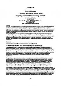
Fig. 2. The progress as a function of time passed for 1000 different MABS (in red) and SD (in blue) simulation runs. See [5] for original coloured document.
Figure 2 illustrates the output of the simulators for 1000 pairs of MABS and SD runs. The vertical axis represents the effort completed or size of artefact (in hours), while the horizontal axis represents the time spent (in hours). Red curves represent MABS simulations, while the blue ones represent SD simulations. It is worth mentioning that for each run, the SD simulation is executed first followed by MABS. Therefore, when a MABS point is plotted on an already existing SD point, that point will turn red, which explains the predominance of red. One can observe that blue
82
R. Cherif and P. Davidsson
Table 2. Result of the statistical analysis of 1000 simulation pairs of MABS and SD runs with varying project scopes drawn at random in the range 100 to 1000 hours Output variable
Duration (Hours) Performance (Effort/Hour,%) Cost (kSEK) Quality (%)
MABS M s 772.24 343.41 72.98 8.66 519.20 240.99 59.82 5.35
SD Analysis M s z value p