Abstract -Software development effort estimation is one of the most major activities in software ... Sudha K.R, Dept of EE,Andhra University,Vizag,AP,INDIA.
87
JOURNAL OF COMPUTING, VOLUME 2, ISSUE 5, MAY 2010, ISSN 2151-9617 HTTPS://SITES.GOOGLE.COM/SITE/JOURNALOFCOMPUTING/ WWW.JOURNALOFCOMPUTING.ORG
Software Effort Estimation using Radial Basis and Generalized Regression Neural Networks Prasad Reddy P.V.G.D, Sudha K.R, Rama Sree P and Ramesh S.N.S.V.S.C Abstract -Software development effort estimation is one of the most major activities in software project management. A number of models have been proposed to construct a relationship between software size and effort; however we still have problems for effort estimation. This is because project data, available in the initial stages of project is often incomplete, inconsistent, uncertain and unclear. The need for accurate effort estimation in software industry is still a challenge. Artificial Neural Network models are more suitable in such situations. The present paper is concerned with developing software effort estimation models based on artificial neural networks. The models are designed to improve the performance of the network that suits to the COCOMO Model. Artificial Neural Network models are created using Radial Basis and Generalized Regression. A case study based on the COCOMO81 database compares the proposed neural network models with the Intermediate COCOMO. The results were analyzed using five different criterions MMRE, MARE, VARE, Mean BRE and Prediction. It is observed that the Radial Basis Neural Network provided better results. Index Terms— Cognitive Simulation, Cost Estimation, Knowledge Acquisition, Neural Nets
—————————— ——————————
1 INTRODUCTION
2. Semi-detached mode – projects that engage teams with a mixture of experience. It is in between organic and embedded modes. 3. Embedded mode – complex projects that are developed under tight constraints with changing requirements. The accuracy of Basic COCOMO is limited because it does not consider the factors like hardware, personnel, use of modern tools and other attributes that affect the project cost. Further, Boehm proposed the Intermediate COCOMO[3,4] that adds accuracy to the Basic COCOMO by multiplying ‘Cost Drivers’ into the equation with a new variable: EAF (Effort 1.1 Intermediate COCOMO The Basic COCOMO model [3] is based on the Adjustment Factor) shown in Table 1. relationship: Development Effort, DE = a*(SIZE)b TABLE 1 where, SIZE is measured in thousand delivered source DE FOR THE INTERMEDIATE COCOMO instructions. The constants a, b are dependent upon Development Intermediate Effort the ‘mode’ of development of projects. DE is measured in man-months. Boehm proposed 3 modes Mode Equation of projects [3]: Organic DE = EAF * 3.2 * (SIZE)1:05 1. Organic mode – simple projects that engage small teams working in known and stable environments. Semi-detached DE = EAF * 3.0 * (SIZE)1.12
I
N algorithmic cost estimation [1], costs and efforts are predicted using mathematical formulae. The formulae are derived based on some historical data [2]. The best known algorithmic cost model called COCOMO (COnstructive COst MOdel) was published by Barry Boehm in 1981[3]. It was developed from the analysis of sixty three (63) software projects. Boehm proposed three levels of the model called Basic COCOMO, Intermediate COCOMO and Detailed COCOMO [3,5]. In the present paper we mainly focus on the Intermediate COCOMO.
Prasad Reddy P.V.G.D,Dept of CSSE,AndhraUniversity,Vizag,AP Sudha K.R, Dept of EE,Andhra University,Vizag,AP,INDIA Rama Sree P,Dept of CSE,Aditya Engg. College,JNTUK,AP,INDIA Ramesh S.N.S.V.S.C,Dept of CSE,SSAIST,JNTUK,AP,INDIA
Embedded
DE = EAF * 2.8 * (SIZE)1.2
88
JOURNAL OF COMPUTING, VOLUME 2, ISSUE 5, MAY 2010, ISSN 2151-9617 HTTPS://SITES.GOOGLE.COM/SITE/JOURNALOFCOMPUTING/ WWW.JOURNALOFCOMPUTING.ORG
The EAF term is the product of 15 Cost Drivers [5] that are listed in Table 2 .The multipliers of the cost drivers are Very Low, Low, Nominal, High, Very High and Extra High. For example, for a project, if RELY is Low, DATA is High , CPLX is extra high, TIME is Very High, STOR is High and rest parameters are Nominal then EAF = 0.75 * 1.08 *1.65*1.30*1.06 *1.0. If the category values of all the 15 cost drivers are “Nominal”, then EAF is equal to 1. TABLE 2 INTERMEDIATE COCOMO COST DRIVERS WITH MULTIPLIERS
S. No
Cost Driver Symbol
1
RELY
0.75
0.88
1.00
1.15
1.40
—
2
DATA
—
0.94
1.00
1.08
1.16
—
3
CPLX
0.70
0.85
1.00
1.15
1.30
1.65
4
TIME
—
—
1.00
1.11
1.30
1.66
5
STOR
—
—
1.00
1.06
1.21
1.56
6
VIRT
—
0.87
1.00
1.15
1.30
—
7
TURN
—
0.87
1.00
1.07
1.15
—
8
ACAP
—
0.87
1.00
1.07
1.15
—
9
AEXP
1.29
1.13
1.00
0.91
0.82
—
10
PCAP
1.42
1.17
1.00
0.86
0.70
—
11
VEXP
1.21
1.10
1.00
0.90
—
—
12
LEXP
1.14
1.07
1.00
0.95
—
—
13
MODP
1.24
1.10
1.00
0.91
0.82
—
14
TOOL
1.24
1.10
1.00
0.91
0.83
—
15
SCED
1.23
1.08
1.00
1.04
1.10
—
Very Very Low Nominal High low high
Extra high
2 PROPOSED NEURAL NETWORK MODELS A neural network [14] is a massive parallel distributed processor made up of simple processing units, which has a natural propensity for storing experimental knowledge and making it available for use. It resembles the brain in two respects [4, 7, 11]: 1) Knowledge is acquired by the network from its environment through a learning process[15] 2)Interneuron connection strengths, known as synaptic weights, are used to store the acquired knowledge. In this section we are going to present the two network models [12] used for the case study i.e. Radial Basis Neural Network(RBNN) and Generalized Regression Neural Network (GRNN).
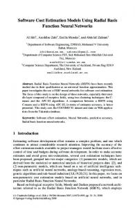
2.1 Radial Basis Neural Network Radial Basis Neural Network (RBNN) consists of two layers: a hidden radial basis layer of S1 neurons, and an output linear layer of S2 neurons [12]. A Radial Basis neuron model with R inputs is shown in Fig. 1. Radial Basis Neuron uses the radbas transfer function. The net input to the radbas transfer function is the vector distance between its weight vector w and the input vector p, multiplied by the bias b. (The || dist || box in this figure accepts the input vector p and the single row input weight matrix, and produces the dot product of the two.)The transfer function for a radial basis neuron is given in (1).
radbas
(n) e n
2
(1)
The 15 cost drivers are broadly classified into 4 categories [3,5]. 1. Product: RELY - Required software reliability DATA - Data base size CPLX - Product complexity 2. Platform: TIME - Execution time STOR—main storage constraint VIRT—virtual machine volatility Fig. 1. Radial Basis neuron model TURN—computer turnaround time A plot of the radbas transfer function is shown in Fig.2. 3. Personnel: ACAP—analyst capability AEXP—applications experience PCAP—programmer capability VEXP—virtual machine experience LEXP—language experience 4. Project: MODP—modern programming TOOL—use of software tools SCED—required development schedule Depending on the projects, multipliers of the cost Fig. 2. radbas transfer function drivers will vary and thereby the EAF may be greater than or less than 1, thus affecting the Effort [5].
89
JOURNAL OF COMPUTING, VOLUME 2, ISSUE 5, MAY 2010, ISSN 2151-9617 HTTPS://SITES.GOOGLE.COM/SITE/JOURNALOFCOMPUTING/ WWW.JOURNALOFCOMPUTING.ORG
The radial basis function has a maximum of 1 when different second layer. its input is 0. As the distance between w and p Fig. 4. Generalized Regression Neural Network Architecture decreases, the output increases. Thus, a radial basis neuron acts as a detector that produces 1 whenever the input p is identical to its weight vector w.The bias b allows the sensitivity of the radbas neuron to be adjusted. RBNN architecture is shown in Fig. 3.
The first layer is just like that for Radial Basis networks. The second layer also has as many neurons as input/target vectors, but here LW{2,1} is set to T. Here the nprod box shown above produces S2 Fig. 3. Radial Basis Neural Network Architecture elements in vector n2. Each element is the dot product of a row of LW2,1 and the input vector a1. The user The output of the first layer of this network net can chooses SPREAD, the distance an input vector must be obtained using (2). be from a neuron's weight. a{1} = radbas(netprod(dist(net.IW{1,1},p),net.b{1})) (2) If you present an input vector to this network, each neuron in the radial basis layer will output a value 2.3 Advantages of Radial Basis Networks according to how close the input vector is to each 1) Radial basis networks can be designed in a fraction of the time that it takes to train standard feed neuron's weight vector. If a neuron has an output of 1, forward networks. They work best when many its output weights in the second layer pass their training vectors are available. values to the linear neurons in the second layer. The second-layer weights LW 2,1 (or in code, LW{2,1}) and 2) Radial Basis Networks are created with zero error on training vectors. biases b2 (or in code, b{2}) are found by simulating the first-layer outputs a1 (A{1}), and then solving the linear expression (3). 3 VARIOUS CRITERIONS FOR ASSESSMENT OF [W{2,1} b{2}] * [A{1}; ones] = T (3) ESTIMATION MODELS We know the inputs to the second layer (A{1}) and the target (T), and the layer is linear. We can use (4) to 1. Mean Absolute Relative Error (MARE) calculate the weights and biases of the second layer to f (RE ) minimize the sum-squared error. (5) MARE (%) 100 Wb = T/[P; ones(1,Q)] (4) f Here Wb contains both weights and biases, with the biases in the last column.There is another factor 2. Variance Absolute Relative Error (VARE) called SPREAD used in the network. The user chooses f ( R E meanR E ) (6) VARE (%) 100 SPREAD, that is the distance an input vector must be f from a neuron's weight. A larger SPREAD leads to a large area around the input vector where layer 1 3. Prediction (n) Prediction at level n is defined as the % of projects neurons will respond with significant outputs. Therefore if SPREAD is small, the radial basis function that have absolute relative error less than n. is very steep, so that the neuron with the weight 4. Balance Relative Error (BRE) vector closest to the input will have a much larger E Eˆ output than other neurons. The network tends to (7) BRE respond with the target vector associated with the min( E , Eˆ ) nearest design input vector. 5. Mean Magnitude of Relative Error (MMRE)
2.2 Generalized Regression Neural Networks A generalized regression neural network (GRNN) is often used for function approximation [8,9]. It has a radial basis layer and a special linear layer.The architecture for the GRNN is shown in Figure 4. It is similar to the radial basis network, but has a slightly
MMRE (%)
1 N MREi 100 N i 1
(8)
90
JOURNAL OF COMPUTING, VOLUME 2, ISSUE 5, MAY 2010, ISSN 2151-9617 HTTPS://SITES.GOOGLE.COM/SITE/JOURNALOFCOMPUTING/ WWW.JOURNALOFCOMPUTING.ORG
ˆ Where MRE E E , N = No. of Projects Eˆ E = estimated effort
Ê = actual effort
Absolute Relative Error (RE) = Eˆ E Eˆ
A model which gives lower MARE (5) is better than that which gives higher MARE. A model which gives lower VARE is better than that which gives higher VARE [6]. A model which gives lower BRE (7) is better than that which gives higher BRE. A model which gives higher Pred (n) is better than that which gives lower Pred (n). A model which gives lower MMRE (8) is better than that which gives higher MMRE. Fig. 5. Actual Effort versus RBNN Effort
4 EXPERIMENTAL STUDY The COCOMO81 database [5] consists of 63 projects data [3], out of which 28 are Embedded Mode Projects, 12 are Semi-Detached Mode Projects, and 23 are Organic Mode Projects. In carrying out our experiments, we have chosen the COCOMO81 dataset[13]. Out of 63 projects, randomly selected 53 projects are used as training data. A Radial Basis Network and Generalized Regression Network are created .The two networks are tested using the 63 dataset. For creating radial basis network, newrbe( ) is used and for creating generalized regression network, newgrnn( ) is used. We have used a SPREAD value of 0.94. The estimated efforts using Intermediate COCOMO, RBNN and GRNN are shown for some sample projects in Table 3. The Effort is calculated in man-months. Table 4 and Fig.5., Fig.6., Fig.7., Fig.8., Fig.9., Fig.10. & Fig. 11. shows the comparisons of various models [10] basing on different criterions.
Fig. 6. Estimated Effort of various models versus Actual Effort
TABLE 4
TABLE 3 ESTIMATED EFFORT IN MAN MONTHS OF VARIOUS MODELS Estimated EFFORT using
Project ID
ACTUAL EFFORT
COCOMO
RBNN
GRNN
1 5 9 29 34 42 47 50 51 52 55 56 58 61
2040 33 423 7.3 230 45 36 176 122 41 18 958 130 50
2218 39 397 7 201 46 33 193 114 55 7.5 537 145 47
2040 33 423 5.6 230 45 62 176 122 41 18 958 130 57
2040 30 345 6.8 188 45 187 151 115 43 16 954 124 88
COMPARISON OF VARIOUS MODELS Model
Intermediate COCOMO
MARE VARE Mean MMRE Pred(40) (%) (%) BRE (%) (%)
19.45
4.97
0.22
18.60
87.3
RBNN
7.13
3.27
0.17
17.29
90.48
GRNN
14.19
4.44
0.35
34.61
84.13
91
JOURNAL OF COMPUTING, VOLUME 2, ISSUE 5, MAY 2010, ISSN 2151-9617 HTTPS://SITES.GOOGLE.COM/SITE/JOURNALOFCOMPUTING/ WWW.JOURNALOFCOMPUTING.ORG
Fig. 10. Comparison of MMRE against various models
Fig. 7. Comparison of MARE against various models
Fig. 11. Comparison of Pred(40) against various models
Fig. 8. Comparison of VARE against various models
5 CONCLUSION Referring to Table 4, we see that Radial Basis Neural Networks yields better results for maximum criterions when compared with the other models. Thus, basing on MARE, VARE, Mean BRE, MMRE & Pred(40) we come to a conclusion that RBNN is better than GRNN or Intermediate COCOMO. Therefore we proved that it’s better to create a Radial Basis Neural Network for software effort prediction using some training data and use it for effort estimation for all the other projects.
REFERENCES [1] [2] Fig. 9. Comparison of Mean BRE against various models [3] [4]
Ramil, J.F, Algorithmic cost estimation for software evolution, Software Engg. (2000) 701-703. Angelis L, Stamelos I, Morisio M, Building a software cost estimation model based on categorical data, Software Metrics Symposium, 2001- Seventh International Volume (2001) 4-15. B.W. Boehm, Software Engineering Economics, Prentice-Hall, Englewood Cli4s, NJ, 1981 Dawson, C.W., “A neural network approach to software projects
JOURNAL OF COMPUTING, VOLUME 2, ISSUE 5, MAY 2010, ISSN 2151-9617 HTTPS://SITES.GOOGLE.COM/SITE/JOURNALOFCOMPUTING/ WWW.JOURNALOFCOMPUTING.ORG
[5]
[6]
[7]
[8]
[9]
effort estimation,” Transaction: Information and Communication Technologies, Volume 16, pages 9,1996. Zhiwei Xu, Taghi M. Khoshgoftaar, Identification of fuzzy models of software cost estimation, Fuzzy Sets and Systems 145 (2004) 141–163 Harish Mittal, Harish Mittal, Optimization Criteria for Effort Estimation using Fuzzy Technique, CLEI Electronic Journal, Vol 10, No 1, Paper 2, 2007 Idri, A. Khoshgoftaar, T.M. Abran, A., “Can neural networks be easily interpreted in software cost estimation?,” Proceedings of the IEEE International Conference on Fuzzy Systems, FUZZ-IEEE’02, Vol.: 2, 1162-1167, 2002 Generalized Regression Neural Nets in Estimating the High-Tech Equipment Project Cost, 2010 Second International Conference on Computer Engineering and Applications, Bali Island, Indonesia March 19-March 21,ISBN: 978-0-7695-3982-9 Mehmet Ali Yurdusev ; Mahmut Firat;Mustafa Erkan Turan “Generalized regression neural networks for municipal water consumption prediction” Published in: Journal of Statistical
[10]
[11]
[12]
[13]
[14] [15]
92
Computation and Simulation , Volume 80, Issue 4 April 2010 , pages 477 - 478 Heiat, A., “Comparison of artificial neural network and regression models for estimating software development effort”, Information and Software Technology 44 (15), 911–922, 2002. Dawson, C.W., “A neural network approach to software projects effort estimation,” Transaction: Information and Communication Technologies, Volume 16, pages 9, 1996 Validating and Understanding Software Cost Estimation Models based on Neural Networks, Ali Idri, Alain Abran, Samir Mbarki 07803-8482-2/04,2004 IEEE Donald J. Reifer, Barry W. Boehm, Sunita Chulani, “The Rosetta Stone: Making COCOMO 81 Files Work With COCOMO II”, CROSSTALK, The Journal of Defense Software Engineering, Feb 1999 Karunanithi, N., et al. “Using neural networks in reliability prediction”, IEEE Software, pp. 53-59, 1992 LiMin Fu, “Neural Networks in Computer Intelligence,” Tata McGraw-Hill Edition 2003, pp.94-97.