Abstract - Underwater Video Spot Detector (UVSD) is a software package designed to analyze underwater video for continuous spatial measurements (path ...
UVSD: Software for Detection of Color Underwater Features Y. Rzhanov, A. Mamaenko Center for Coastal and Ocean Mapping, Univ of New Hampshire, NH M. Yoklavich NOAA NMFS SWFSC, Santa Cruz Laboratory, CA
planar surface perpendicular to the beams is equal to a distance between the lasers. These projections appear in an image taken by a camera as bright distinct spots (which will be called laser dots in this paper). When the imaged surface (seafloor, in our case) is at an infinite distance from the camera, laser dots converge to a single point (vanishing point). The position of this point within an image frame depends on mutual orientation of the camera and lasers. Distance between the camera and seafloor is uniquely identified by a distance between a laser dot and a vanishing point (or equivalently, a distance between laser dots). Recent advances in using this technology are described in [1-4].
Abstract - Underwater Video Spot Detector (UVSD) is a software package designed to analyze underwater video for continuous spatial measurements (path traveled, distance to the bottom, roughness of the surface etc.) Laser beams of known geometry are often used in underwater imagery to estimate the distance to the bottom. This estimation is based on the manual detection of laser spots which is labor intensive and time consuming so usually only a few frames can be processed this way. This allows for spatial measurements on single frames (distance to the bottom, size of objects on the sea-bottom), but not for the whole video transect.
Detection of laser dots in underwater images, however, is not a simple task. Watching footage with laser dots in a view, human rarely has problems with their detection. Even if an eye loses such a feature, it is easily picked up again after few frames. Given any single frame without an advantage of knowing the approximate position of laser dots makes the detection task significantly more difficult.
We propose algorithms and a software package implementing them for the semi-automatic detection of laser spots throughout a video which can significantly increase the effectiveness of spatial measurements. The algorithm for spot detection is based on the Support Vector Machines approach to Artificial Intelligence. The user is only required to specify on certain frames the points he or she thinks are laser dots (to train an SVM model), and then this model is used by the program to detect the laser dots on the rest of the video.
We have developed an approach where predictive power of human brain compliments robustness and repeatability of a computer. The human operator is training an artificial intelligence scheme on few chosen frames, and this scheme is then used to process the rest of the video footage.
As a result the precise (precision is only limited by quality of the video) spatial scale is set up for every frame. This can be used to improve video mosaics of the sea-bottom. The temporal correlation between spot movements changes and their shape provides the information about sediment roughness. Simultaneous spot movements indicate changing distance to the bottom; while uncorrelated changes indicate small local bumps.
II. PREPROCESSING: LENS CORRECTION Prior to processing all the footage undergoes lens correction procedure. This correction is not essential for the subject of this paper, but is usually important for accuracy of measurements, which are the final goal for the whole project. The correction is based on a set of camera-specific parameters determined in a calibration procedure, described in [5].
UVSD can be applied to quickly identify and quantify seafloor habitat patches, help visualize habitats and benthic organisms within large-scale landscapes, and estimate transect length and area surveyed along video transects.
I. INTRODUCTION
III. CLASSIFICATION
Determination of scales, sizes and distances of various objects from underwater imagery is an important issue in underwater habitat biology, geology, archaeology, cable laying industry, etc., where contact measurements cannot be done straightforwardly. To aid with this task, lasers are often used.
A. Support Vector Machines Automation of laser spots detection is done using an artificial intelligence learning system known as Support Vector Machine (SVM) [6, 7]. Recently SVM classifiers have attracted much attention due to relative simplicity in application and good results achieved in a variety of problems. SVMs are designed to solve two-class problems (as is the one discussed in this paper).
A simple setup includes two or more lasers with parallel beams, approximately parallel to a camera optical axis. In this setup, distance between projections of laser beams on a
1
SVM is an apparatus to classify the input data according to a decision model developed during a user-supervised training. Data points, crucial for classification, that are selected by SVM, form a basis of support vectors, which determine a decision surface – hyper-plane in the feature space separating data points with different class membership. The training process allows for choosing interactively data points leading to an optimal separation between two different classes.
IV. DETECTION A. Pixel Processing During the classification stage, each pixel is classified by SVM in one of two categories: as either a part of a laser dot or not. Obviously there is no need to classify each and every pixel in acquired images - laser dots may appear in a video frame only along straight lines that are projections of laser beams onto retinal plane of the image (beam lines). Taking these simple geometrical constraints into consideration not only saves the processing time, but also allows to avoid a multitude of false positives often appearing in a near field, where intense illumination causes colors to saturate (Fig.1).
The user chooses few frames from video footage and within each frame selects a rectangular area (or areas) with laser dots. Pixels in these areas (active zones) are manually classified into one of two classes: as part of a laser dot, or as part of a background. All pixels within active zones constitute data for the training process, each pixel being a vector in a 3-dimensional color space: RGB, HSL, or other. The size of training set is a tradeoff between model accuracy and its generality. We have found that the best results are achieved when the dimension of an active zone is approximately three or four times larger than the laser dot diameter.
In principle, precise knowledge of camera and laser setup allows for calculation of beam lines, but a small error in an angle measurement may lead to a much larger error in their predicted parameters, so in practice it is simpler to determine these parameters directly from the footage by means of image processing. All the acquired frames, corrected for the lens distortion (even weak distortion may preclude beam lines from being straight), are stacked (Fig. 2.), and tiny reflections of laser light from particles suspended in water column form bright belts showing where the beam lines are. This approach works reliably even in a very clear water for a sufficiently long frame sequence.
Fig. 1. Results of the classification of an entire frame (notice that the digits at the top of the frame were classified as laser dots too).
The SVM-based approach allows for using in classification not only brightness of pixels, as has been done in earlier work, but also their color, which increases robustness of detection.
Fig. 2. An example of stacking video frames in a movie.
The developed application allows for automatic detection of beam lines from the stacked image (based on assumptions that number of beams is known, and the vanishing point is near the middle of a frame), but it is often simpler for the user just to point-and-click on ends of beam lines, and these parameters are then used in the processing. The user also can specify the width (in pixels) of the belts around beam lines where the laser dots will be searched for. The example of detection with these constraints taken into account is presented in Fig. 3.
B. Iterative Approach to Training Appearance of laser dots change from frame to frame due to changing conditions: seafloor sediment, water clarity, distance from lasers to seafloor, etc. This requires an iterative approach – initially trained SVM model is used for processing of video footage, then the user decides which frames were processed poorly, and uses these frames for model refinement. Occasionally, when visual conditions change dramatically within a single footage, multiple refinements may lead to model over-fitting – the only solution for this seems to be the use of different SVM models for different parts of the footage.
There is also an important application when the above mentioned constraints are not essential. When video frames have to undergo registration process (for example, for construction of video mosaic), bright laser dots act as strong
2
clarity. The most popular video compression algorithms such as MPEG, DV, etc., reduce the size of video by discarding information not important for casual human perception. However the important color information is being lost at the process. Clarity of water is responsible for scattering. The more turbid is the water, the more false blobs appear due to scattering. One of the possible ways to improve results is to use green laser, as its light scatters less in water. The example of detection is presented in Fig. 5.
features that seriously hinder the registration process. To remove these features, pixels that form laser dots are detected in the same way as described above and then simply replaced by pixels colored with background colors. There is no need to detect blobs (as is done below); pixels in the area around laser dots are classified using SVM, and all the pixels that are classified positively are replaced by other pixels randomly drawn from the negatively classified pool.
Fig. 3. An example of pixel classification with geometrical constraints applied (greenish pixels were classified as parts of laser dots)
B. Pixel Processing Once individual pixels are classified, they could be joined in clusters representing potential locations of laser dots. Often these clusters are dense and straightforward calculation of their centroid provides a reasonable estimate for laser dot location (Fig. 4, a-b). With a poor SVM model (due to changing visual conditions) clusters have holes and/or complex shapes (Fig. 4, c-d). The application of morphological operations (closing) helps to improve the cluster shape.
Fig. 4. Examples of pixels classified as laser dots. a), b) show good detection, c), d) inadequate detection. An example of pixel classification with geometrical constraints applied (pixels that had been classified as parts of laser dots were colored bright green).
VI. UNDERWATER VIDEO SPOT DETECTOR GUI Once the laser dots are detected in separate frames, their locations can be considered as a function of time. It is reasonable to assume that the distance from the camera to the seafloor is changing slowly. Hence location of a laser dot in an image frame must be changing slowly as well, so large jump indicates either that the dot location was detected incorrectly, or that the laser beam was intercepted by some object far away from the seafloor (for example, blade of grass). In both cases this data point is considered to be an outlier and is rejected.
Laser light propagating in water is affected by two major phenomena: absorption and scattering. With the distance traveled, the former decreases brightness of laser beam and the latter increases its diameter. Scattering on particles suspended in water column results in appearance of several bright spots along the beam (which in fact allows for detection of beam lines, described above). These processes are discussed in details in, for example, [4, 8]. Typically it is desirable to detect an intersection of laser beam with an object that does not allow the light to propagate any further. Hence in the case of several detected blobs along the same beam line, the algorithm chooses the blob closest to the vanishing point.
Robust outlier detection is implemented using RANSAC algorithm [9]. Sequence of laser dot locations is chosen to represent 3 seconds (i.e. with 3 frames per second is 9 frames long). At every step two data points are chosen randomly, a linear model is built, and other points are checked against the model. Number of tries is chosen sufficiently high, to guarantee that at least one of linear models has been built from uncontaminated data. The estimate of this number is calculated using the formula from [10]. The solution with the lowest standard deviation of inlying residuals is chosen, and
V. EXPERIMENTAL RESULTS In our experiments we have trained the model and performed detection in RGB color space. Experiments have shown that in this case the robustness of laser dots detection is mostly affected by video data compression and water
3
Acknowledgments
the data points lying further than 5 pixels from the line representing the best solution are considered to be outliers.
Y. R. and A. M. would like to thank Dr Lloyd Huff for many invaluable discussions. This work was supported by NOAA grant NA97OG0241. References [1] M. Caccia, “Optical Triangulation-Correlation Sensor For Underwater Vehicles’ Motion Estimation”. Proceedings of the 10th Mediterranean Conference on Control and Automation - MED2002 Lisbon, Portugal, July 9-12, 2002. [2] D. M. Kocak, T. H. Jagielo, F. Wallace, J. Kloske, “Remote Sensing using Laser Projection Photogrammetry for Underwater Surveys”, IGARSS’04 Proceedings, September 2004. [3] D. M. Kocak, F. M. Caimi, T. H. Jagielo, J Kloske, “Laser Projection Photogrammetry and Video System for Quantification and Mensuration”, Oceans’2002 Proceedings, pp.1579-1574. [4] J. S. Jaffe, “Sensing Plankton: Acoustics and Optical Imaging”, (book chapter), European Workshop on Harmful Algal Blooms, (to appear) 2005. [5] J.-Y. Bouguet, Camera Calibration Toolbox for MATLAB, http://www.vision.caltech.edu/bouguetj/calib_doc [6] V. N. Vapnik, "Statistical learning theory." 1998, John Wiley & Sons. [7] N. Cristianini, J. Shawe-Taylor, "An introduction to Support Vector Machines and other kernel-based learning methods." Cambridge University Press, 2000. [8] E. P. Zege, A. P. Ivanov and I. L. Katsev, “Image Transfer Through a Scattering Medium”, Springer Verlag, New York, 1991. [9] M. A. Fischler, R. C. Bolles, “Random sample consensus: A paradigm for model fitting with applications to image analysis and automated cartography”. CACM, 24 (6): 381-395, 1981. [10] P J Rousseeuw, “Robust regression and outlier detection”, Wiley, New York, 1987.
a)
350
300
Distance, (pixels)
250
200
150
100
50
0 200
400
600
800
1000 Frame Number
1200
1400
1600
1800
b) Fig. 5. An example of a low quality video a) and results of its processing b). Both water quality and compression problems (near field saturation) present challenges to the algorithm.
The gaps in the data due to undetected laser dots or rejected outliers are filled in using quadratic interpolation (higher degrees may lead to over-fitting). One of the applications that stimulated the development of this software was the need to estimate distance traveled by a submersible from video footage taken from the vehicle. Detailed description of the technique will be published elsewhere; here we will just outline it. Sequential frames from video footage (possibly sub-sampled) are co-registered using simple translational model. This provides an estimate of traveled distance (in a period of time between these two frames) in pixel space. This space, however, can be related to a real space using the information obtained from laser dots processing. Estimates of traveled distance (around 10 minutes at 2 knots speed) obtained with this technique were compared with three other independent estimates, and were found to be always within the range between the lowest and highest bounds.
4