Software Reliability Modeling With Different Type of Faults Incorporating Both Imperfect Debugging and Change Point Subhashis Chatterjee, Ankur Shukla Department of Applied Mathematics, Indian School of Mines, Dhanbad, India 1
[email protected] 2
[email protected]
Abstract— In past four decades, many nonhomogeneous Poisson process (NHPP) based software reliability growth models (SRGMs) have been proposed to measure and assess the reliability growth of software. During the testing process, the faults which causes failure are detected and removed. One common assumption of many traditional SRGMs is that the fault removal rate is constant. In practical, the fault removal rate increases with time as learning and maturity of software engineer increases. Hence, time variant fault removal rate has been considered in this study. A complex software system may contain different category of faults. Some of faults can be easily detected and removed and some of faults required more effort to be detected and removed. Therefore, in this article, a NHPP based SRGM has been proposed which incorporates mainly two type of faults, major and minor. The concepts of imperfect debugging and change point have also been incorporated in the proposed SRGM. The parameters of the proposed SRGM is estimated using Statistical Package for Social Sciences (SPSS) software and validation of the proposed SRGM has been done using real life data set. Keywords— Non-homogeneous Poisson process; Software reliability; Software reliability growth model; Imperfect debugging; Change point
I. INTRODUCTION In this fast changing world, with the rapid growth of technology a remarkable change has been taken place in the area of computer science. This development in the area of computer science has made the modern society more computer dependent. Software plays a major role in functioning of a computer. Therefore, in this automated world, the demand of quality software is increasing for safe performance of any automated system. Accordingly, it becomes the great concern to control and maintain the reliability of the software for the software industries. According to Musa [1], `Software reliability is defined as the failure-free operation of a software under specified environment and specified time'. The reliability of software can be measured by SRGMs. SRGMs are developed based on failure data obtained during software testing phase. In past four decades, many SRGMs considering different assumptions and concepts, have been developed to estimate the reliability growth of the software products during the development
978-1-4673-7231-2/15/$31.00 ©2015 IEEE
process [2-12]. One such assumptions is, fault removal rate is, constant during the testing process [3, 4, 5, 8, 13-14]. In reality, it is observed that fault removal rate can't be constant, it changes due to change in testing strategy, testing skill, testing effort, complexity and size, defect density, etc. [8]. Actually, fault removal rate increases with time as learning and maturity of software engineers increases, and become constant at the end of the testing process [5, 8, 15]. On the other hand, different types of faults may be possible in a complex software system. It is very important to measure the characteristics and severity of the faults to improve the fault removal process. Therefore, this issue should be taken into consideration to study the behaviour and severity of faults. The faults present in a software can be classified as major and minor faults. Minor faults are those faults which can be easily detected and removed, and major faults are those faults which are difficult to detect and remove. Hence, it is obvious that major faults require more effort to be detected and removed compare to the minor faults. Initially, fault removal rate of major faults are less in compare to the minor faults, which may become similar to the minor faults at the end of testing [5, 8]. Due to effect of different factors like testing environment, testing strategy, testing team constitution and efficiency, test case effectiveness, resources, etc., fault removal rate and fault introduction rate get affected and they changes when above factors are changed. These points at which changes are possible is known as ‘change point’. Various SRGMs on the concept of change point have been proposed by many researchers in past few years [8, 16-19]. Previously, Many SRGMs has been proposed considering that the debugging process is perfect, i.e., no fault will be spawned. But in reality, it is observed that faults may be introduced when detected faults are removed during the debugging process. This process is known as imperfect debugging. Considering this phenomenon many SRGMs has been developed [4, 5, 8, 17, 20]. The concept of imperfect debugging has also been incorporated in the proposed SRGM. In this paper, a NHPP based SRGM has been developed considering two types of faults based on severity. In addition, imperfect debugging phenomenon has been considered with fault introduction and time dependent fault removal rate.
Different fault removal and introduction rate has been considered for different types of faults to analyse the realistic behaviour of the faults. Furthermore, to study the effect of different factors such that: testing strategy, testing environment, testing effort, resource allocation, the concept of change point has been considered for different parameters. Rest of the article is organised as follows: The assumption and formulation of the proposed SRGM in section 2. Parameter estimation of proposed SRGM and different comparison criteria are presented in section 3. Numerical analysis and model validation has been done in section 4. Finally, section 5 concludes the work.
⎧⎪bi1 (1 − qi1t − ri1 ), 0 ≤ t ≤ τ bij (t ) = ⎨ −r ⎪⎩bi 2 (1 − qi 2 t i 2 ), t > τ
where bij , qij , rij are constant and defined for i t h type 5.
[m(t )]n exp(−m(t )), n = 0,1, 2 … n! dm(t ) λ (t ) = = b(a − m(t )) dt
P[N(t)=n] =
⎧ βi1 , 0 ≤ t ≤ τ ⎩ βi 2 , t > τ
t
0
(5)
where βij is constant and defined for i t h type of faults in j t h interval and τ is the change point. From the above assumptions the mean value function for i t h type of faults mi (t ) can be obtained solving the following differential equations:
dmi (t ) = bij (t ){ai (t ) − mi (t )} (6) dt dai (t ) dm (t ) = β ij (t ) i (7) dt dt (1) where ai (t ) is the number of i t h type of faults to be (2) eventually detected. The above equations satisfy the initial conditions ai (0) = api and mi (0) = 0, pi is the proportion of
where a denotes the total number of faults present in software before testing and b denotes the proportionality constant which is defined as fault removal rate. Mean value function, m(t ) , can be defined as: m(t ) = ∫ λ (t )dt
of faults in j t h interval and τ is the change point. Due to imperfect debugging new faults are introduced with fault introduction rate βij (t ), which is different for different type of faults, defined as:
βij (t ) = ⎨
II. MODEL DEVELOPMENT This section gives a brief idea about NHPP based SRGMs and proposed SRGM. A. NHPP Based SRGMs Let N(t) be a counting process representing the cumulative number of faults at time t with the mean value function, m(t ) , which represent the s-expected number of faults by time t. Goel-Okumoto [13] proposed a SRGM by assuming that N(t) follows NHPP and the failure intensity λ (t ) is proportional to the number of remaining faults, i.e.,
(4)
(3)
Many SRGMs are proposed with the assumptions of GoelOkumoto SRGM [3-5, 8]. The proposed SRGMs has been also integrated the above assumptions. B. Proposed SRGM The proposed SRGM has been developed considering the following assumptions: 1. Software failure follows NHPP. 2. The Software system is subjected to failure caused by remaining faults in the system. 3. Debugging process is imperfect, i.e., it is possible to introduce new faults when detected faults are removed. 4. Fault removal rate increases with time as learning process, testing effort, etc., increases. It is different for different type of faults and it will change due to change in environmental factor, resource allocation, etc. Hence, the fault removal rate bij (t ) will be as follows:
i t h type of faults. Since, fault removal rate can't be negative, hence r (8) 1 − qij t ij > 0
i.e.
1/ rij
t > (qij )
Hence, this condition must be considered in parameter estimation also. C. Solution of the Proposed SRGM Solving the Eqn. (6) and (7) simultaneous with initial conditions ai (0) = api and mi (0) = 0 , we can find the mean value function of the different fault given as follows: 1.
2.
Minor Faults (for i = 1 ) Case I. For 0 ≤ t ≤ τ mean value function has been shown in eqn. (9) Case II. For t > τ mean value function has been shown in eqn. (10) Major Faults (for i = 2 ) Case I. For 0 ≤ t ≤ τ mean value function has been shown in eqn. (11) Case II. For t > τ mean value function has been shown in eqn. (12)
m1 (t ) =
⎛ ap1 q11 1− r11 ⎞ ⎪⎫⎤ ⎡⎣1 − exp {− (1 − β11 ) b11 ⎜ t − t ⎟ ⎬⎥ (1 − β11 ) ⎝ (1 − r11 ) ⎠ ⎭⎪⎦⎥
m1 (t ) =
⎡ ⎛ ⎞ ⎛ q ⎞ ⎪⎫⎤ ap1 q ⎪⎧ 1 ⎢1 − exp ⎨b11 (1 − β11 ) ⎜τ − 11 τ 1− r11 ⎟ + b12 (1 − β12 ) ⎜ 12 t1− r12 − τ 1− r12 − (t − τ ) ⎟ ⎬⎥ (1 − β12 ) ⎢⎣ ⎝ 1 − r11 ⎠ ⎝ 1 − r12 ⎠ ⎭⎪⎥⎦ ⎩⎪
(
+ m(τ )
)
( β11 − β12 )
⎧⎪ ⎛ ap2 ⎡ q21 1− r21 ⎞ ⎫⎪⎤ t ⎢1 − exp ⎨ − (1 − β 21 ) b21 ⎜ t − ⎟ ⎬⎥ (1 − β 21 ) ⎢⎣ ⎝ (1 − r21 ) ⎠ ⎭⎪⎦⎥ ⎩⎪
m2 (t ) =
⎛ ⎛ q ⎞ ⎪⎫ ⎤ ap2 ⎡ q ⎪⎧ 1− r ⎞ 1− r 1− r ⎢1 − exp ⎨−b21 (1 − β 21 ) ⎜τ − 21 τ 21 ⎟ + b22 (1 − β 22 ) ⎜ 22 t 22 − τ 22 − (t − τ ) ⎟ ⎬ ⎥ (1 − β 22 ) ⎣⎢ ⎪⎩ ⎝ 1 − r21 ⎠ ⎝ 1 − r22 ⎠ ⎪⎭ ⎦⎥
)
( β 21 − β 22 )
(12)
(1 − p2 β 22 )
m(t ) = ∑ mi (t ) i
III. PARAMETER ESTIMATION AND COMPARISON CRITERIA A. Parameter Estimation Least Square method is used to estimate the parameters. The estimated values has been obtained using SPSS. The position of change point is found using `changepoint' package in `R' software [21]. B. Comparison Criteria Following comparison criteria has been performance analysis of the proposed SRGM.
used
for
1 n ∑ (yi − yˆi )2 n i =1
where yi and yˆ i are the observed and predicted faults respectively, n is the total number of observations. 2. Bias It is defined as the sum of the deviation of the estimated curve from the actual data, defined as [22, 23]: 1 ∑ (m(tk ) − mk ) n k =1
smaller value of bias is better goodness of fit. 3. Variance It is defined as follows [22, 23]: 1 n ∑ (mk − m(tk ) − Bias)2 n − 1 i =1 smaller value of variance is better goodness of fit. Variance =
4. Root Mean Square Prediction Error It measure the closeness with which a model predicts the observation, as shown [22, 23]:
RMSPE = Variance2 + Bias 2
1. Mean Square Error (MSE) It is defined as [4, 5]:
n
(11)
(
D. Mean Value Function of the Proposed SRGM The mean value function of the proposed SRGM is defined as follow:
MSE=
(10)
(1 − β12 )
m2 (t ) =
+ m(τ )
Bias =
(9)
lower value of RMSPE is better goodness of fit. 5. The 100p% Upper and Lower Limit for m(t) It is defined as follows [24]:
mˆ (t ) + η p mˆ (t ) and mˆ (t ) − η p mˆ (t ) The bounds of m(t ) approximately as follows:
mˆ (t ) + η p mˆ (t ) = m(t ) = mˆ (t ) − η p mˆ (t ) where mˆ (t ) is the estimate of m(t ) and η p is the percent point of the standard.
(1 + p ) × 100 2
IV. NUMERICAL ANALYSIS AND MODEL VALIDATION The data set used here for validation of the proposed SRGM has been taken from the article published by Ohba [25]. This data set consists of 328 software faults during 19 weeks. The change point for this data set is found at the position 8th , 10th and 13th week. Let p1 = p, since
p1 + p2 = 1 ⇒ p2 = 1 − p, considering this the estimated values of the parameters of the proposed SRGM and other SRGM has been shown in Table 1.
As shown in Table I, it is clear that fault removal rate for minor faults is greater than the major faults and it increases after change point and fault introduction rate for both type of fault is decreases after change point. This establishes the fact that more testing effort is required to remove the major faults than the minor faults from the system. The estimated total number of faults by proposed SRGM is 328.03 which is very close to the actual number of faults i.e. 328. Hence, from the above results it clear that the assumptions of the proposed SRGM is realistic.
TABLE 1. Estimated parameters of Some Existing SRGMs.
400 Estimated faults Actual faults 95% confidence upper bound 95% confidence lower bound
350
Estimated Parameters of Different Models
300
a
p
b11
b12
b21
b22
328.04
0.655
0.309
1.160
0.078
0.185
β11
β12
β21
β22
r11
r12
0.354
0.269
0.256
0.007
2.615
0.969
r21
r22
q11
q12
q21
q22
0.401
1.007
0.052
7.164
0.020
0.798
Kapur et al. model
a
p1
p2
b1
b2
b3
329.03
0.604
0.268
0.089
0.061
0.002
Cumulative faults
Proposed Model
250 200 150 100 50 0
0
2
β1
β2
α1
α2
333.32
0.0002
0.0005
0.2119
0.0094
0.091
0.002
Shyur Model
a
b1
b2
β1
β2
330.00
0.092
0.114
0.267
0.604
10 time
12
14
16
18
20
Proposed Model Kapur et al. Model Chatterjee et al. Model Shyur et al. Model Actual Faults
250 Cumulative Faults
b2
8
350
300
b1
6
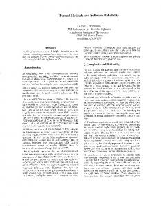
Fig. 1. Estimated cumulative faults using proposed model and the 95% confidence bounds versus time.
Chatterjee et al. Model
a
4
200
150
100
50
TABLE 2. Comparison of the Proposed Model with different existing SRGMs
0
2
4
6
8
10 Time (t)
12
14
16
18
20
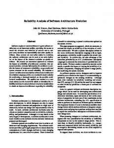
Fig 2. Graphical comparison of the proposed SRGM with other existing SRGM
Comparison Criteria Models
0
MSE
Bias
Variance
RMSPE
Proposed Model
36.993
0.0758
6.081
6.082
Kapur Model
133.35
-0.7439
11.839
11.863
Chatterjee Model
106.56
0.4504
10.595
10.605
Shyur Model
122.94
0.3483
11.386
11.392
From the Table II, it is clear that the MSE, Bias, Variance, RMSPE of the proposed SRGM is lower in comparison to the other SRGMs [17, 15, 19], which shows that the performance of the proposed SRGM is better in compare to the other SRGMs [17, 15, 19]. Graphical representation of the cumulative number of faults estimated by the proposed SRGM has been shown in Fig. 1 and from
this figure it is clear that the pattern of the estimated faults are very close to the actual faults present in the software. It means no faults are present in the software at end of the testing. Hence, proposed SRGM is better fit for given data set. Fig. 2 represents the graphical comparison of the proposed SRGM with the other existing SRGMs. V. CONCLUSION In this paper, a SRGM has been proposed with new time dependent fault removal rate incorporating both the concept of change point and imperfect debugging. Effect of different types of faults on fault removal rate and fault introduction rate has been shown. The proposed model is more realistic and flexible. Real data has been used to validate the proposed model. Experimental results established the fact that, the proposed model has better and accurate prediction capability. Hence, the proposed models can be very helpful for industry and software professionals to improve the quality of software.
[14] [15]
[16] [17] [18] [19]
[20] [21] [22] [23]
ACKNOWLEDGMENT Authors acknowledge Indian School of Mines, Dhanbad, India, for providing necessary facilities for this work.
[24]
[25]
REFERENCES [1] [2] [3] [4] [5] [6] [7] [8] [9] [10] [11]
[12]
[13]
J. D. Musa, A. Iannino and K. Okumoto, Software Reliability, Measurement, Prediction and Application, McGraw-Hill, New York, 1987. J. D. Musa, A Theory of Software Reliability and Its Application, IEEE Transactions on Software Engineering, SE-1(3), 1975, 312-327. M. Xie, Software Reliability Modeling, World Scientific, Singapore, 1991. M. R. Lyu, Handbook of Software Reliability Engineering, McGrawHill, New York, 1996. H. Pham, Software Reliability, Springer-Verlag, 2000. X Zhang, M.Y. Shin and H. Pham, Exploratory analysis of environmental factors for enhancing the software reliability assessment, J Syst Softw, 2001, 57, 73-78. Y. K. Malaiya, M.N. Li, J.M. Bieman, R. Karcich, Software reliability growth with test coverage. IEEE Trans Reliab, 2002, 51(4), 420-426. P. K. Kapur, H. Pham, A. Gupta and P.C.Jha., Software Reliability Assessment with OR application, Springer, 2011. S. Chatterjee, S. Nigam, J.B. Singh and L.N. Upadhyaya, Transfer Function Modeling in Software Reliability, Computing, 2011, 92(1), 33-48. S. Chatterjee, S. Nigam, J.B. Singh and L.N. Upadhyaya, Software Faults Predication Using NARX Network, Applied Intelligence, 2012, 37(1), 121-129. S. Chatterjee, S. Nigam, J.B. Singh and L.N. Upadhyaya, An Improved Additive Model for Reliability Analysis of Software with Modular Structure, Journal of Applied Mathematics and Informatics, The Korean Society for Computational and Applied Mathematics, 2012, 30(3), 489 - 498. S. Chatterjee and J.B. Singh, A NHPP based software reliability model and optimal release policy with Logistic-Exponential test coverage under imperfect debugging, International Journal of Systems Assurance Engineering and Management, 2014, 5(3), 399-406. A. L. Goel, K. Okumoto, A time dependent error detection rate model for software reliability and other performance measures, IEEE Trans. Reliab, 1979, 28, 206-211.
S. Yamada, M. Ohba and S. Osaki, S-shaped reliability growth modeling for software error detection. IEEE Trans. Reliab, 1983, 12, 475-484. P. K. Kapur, Archana Kumar, Kalpana Yadav, S.K. Khatri, Software reliability growth modelling for errors of different severity using change point, International Journal of Reliability, Quality and Safelty Engineering, 2007, 14(4), 311-326. M. Zhao, Change-point problems in software and hardware reliability. Commun. Stat.-Theor. Method, 1993, 22(3), 757-768. H.J. Shyur, A stochastic software reliability model with imperfect debugging and change-point, J. Syst. Softw, 2003, 66(2), 135-141. F. Z. Zou, A change-point perspective on the software failure process. Software testing Verif. Reliab, 2003, 13(2), 85-93. S. Chatterjee, S. Nigam, J.B. Singh and L.N. Upadhyaya, Effect of change point and imperfect debugging in software reliability and its optimal release policy, Mathematical and Computer Modelling of Dynamical Systems, 2012, 1-13. H. Pham, Software reliability assessment: Imperfect debugging and multiple failure types in software development, EG&GRAMM- 10737, Idaho National Engineering Laboratory, 1993. R. Killick and I. Eckley, changepoint: An R package for Change point Analysis, Journal of Statistical Software, 2014, 58(3), 1-19. K. Pillai and V.S.S. Nair, A model for software development effort and cost estimation. IEEE Trans. Softw. Eng., 1997, 23(8), 485-497. C. Y. Huang and S.Y. Kuo, Analysis of incorporating logistic testing effort function into software reliability modeling, IEEE Trans. Reliab, 2002, 51(3), 261-270. L. Yin and K.S. Trivedi, Confidence interval estimation of NHPPbased software reliability models In: Proceedings of the 10th International Symposium on Software Reliability Engineering, 1999, pp. 6-11. M. Ohba, Software reliability analysis models, IBM Journal of Research and Development, 1984, 28 (4), 428-443.