Software Reliability Nonlinear Modeling and Its Fuzzy ... - CiteSeerX

4th WSEAS Int. Conf. on NON-LINEAR ANALYSIS, NON-LINEAR SYSTEMS and CHAOS, Sofia, Bulgaria, October 27-29, 2005 (pp49-54)

Software Reliability Nonlinear Modeling and Its Fuzzy Evaluation GUO JUNHONG1,2, YANG XIAOZONG1, LIU HONGWEI1 School of Computer Science and Engineering 1 Harbin Institute of Technology Harbin, Xidazhi street No.92 150001 School of Computer Science and Technology 2 Heilongjiang University Harbin, Xuefu road No.74 150080 CHINA

Abstract: - Based on the research of the present developing situation in software reliability models, this paper found that it was difficult to satisfy the hypothesis condition of models in actual projects, and these hypothesis restrict the universality of those models. However, the testing data satisfies the properties of time series. This paper presents a nonlinear model of software reliability based on time series and gives corresponding algorithms. The simulation experiments show the accuracy and efficiency of this new model. The newly proposed model suits the requirement of software engineering better and its parameters can reflect the changing of software reliability. The new model can have more accurate analysis and forecast to software reliability issue without any strict assumption. Furthermore, the fuzzy theory is introduced to evaluate software reliability. Using the fuzzy theory that integrated the fuzziness and randomness, the software reliability evaluation method is more approaching to the real system and the accuracy of software reliability evaluation is promoted greatly. Keywords: - Software reliability nonlinear model; Time series analysis; Software reliability growth model; Software reliability evaluation obtain accurate software reliability estimation, it requires a large number of failure data which are not usually available until the system has been tested for a long relative period. Many software reliability engineers are more interested in estimating the software reliability as early as possible [3]. This paper proposes a method for early and more accurate software reliability prediction by time series analysis. Its calculation methods are simple and without any strict assumption. This paper is organized as follows. Section 2 presents the state of software reliability modeling. Section 3 shows the feasibility of software reliability nonlinear modeling based on time series. The implemented algorithm is given in section 4. Section 5 provides the simulation analysis of testing data. In section 6, fuzzy theory are used to evaluate software reliability. Finally, a brief conclusion is presented.

1 Introduction Due to the complexity of computer software systems and the increasing of development cost, it is of utmost importance to develop high quality software systems. The quality of the software system is described by many metrics such as: complexity, maintainability, availability, reliability, etc. As tragedies of unreliable software often take place, people recognize the importance of developing reliable software. Now, the reliability problem in software systems is a well-known research field.Therefore, designing reliable software and evaluation software reliability accurately are the most important issues [1]. The standard definition of reliability for software (Musa, Iannino, and Okomoto, 1987) is the probability of execution without failure for some specified interval of natural units or time [2]. Software failures are the manifestation of software errors which are introduced into the software by software engineers during the phases of software development cycle. In the literatures, researchers establish software reliability growth model (SRGM) to measure software reliability. To apply these models, it is necessary to know how well the models suit an actual observation failure data set. In order to

2 The State of Software Reliability Modeling SRGM is defined as the mathematical relationship between the number of software errors removed and testing time. Classical SRGMs have great influence 1


on software reliability modeling research. In spite of the fact that many software reliability growth models have been proposed in the software reliability literature since the first one appeared in 1972 [4], no one of them can deal properly with all possible situations. According to the software error removal process, Jelinski and Moranda proposed the first model. The model has a simple structure and assumptions. Then Musa proposed the Basic Execution Time Model which has similar assumptions to those of Jelinski and Moranda(J-M) model [5]. J-M model made a major contribution to the understanding the relation of error removal and software execution time. Goel-Okumoto model is the first nonhomogeneous Poisson process(NHPP) SRGM. Goel-Okumoto model assumed that the error removal process follows NHPP. The assumption of this model is similar to the Basic Execution Time model of Musa [6]. Those models are mainly based on some assumption conditions and believe that SRGM has been established according to a certain probability process. The assumptions are the key factors of establishing SRGM. There is a relation between assumptions chosen and modeling success. But in practical application, quite a few assumptions are unfit to software developing process, which can not be accepted by most people, thus limiting the application of the models. Using this kind of model can even get the unimaginable parameter under some conditions. Furthermore, a software failure data set being evaluated can get different results by using different models. So it has reached a common viewpoint in software reliability evaluation field, in that there isn’t a “good model” that can fit all failures data very well [7]. J-M model assumes that all errors that have been checked in the test can be eliminated and removes one error each time. Removing one error does not affect the remaining errors. But in fact, software development and error removal are all human behaviors, which are unpredictable, so it can not avoid of introducing new errors during the process of error removal. Goel-Okumoto model suppose that each error is independent, each error has the same probability of leading system failure and each failure interval time is independent. Sometimes, modules in software program have some relations, so it is impossible to have complete independence, and the probability of each failure that causes system failure is not the same [8,9]. In these three models, the cumulative numbers of errors removal grow exponentially with the testing time. The exponential growth curve is due to the

assumption that the error removal intensity is linearly related to the remaining number of software errors [10]. In many software development projects it was observed that the relation between the cumulative numbers of errors removed and the testing time is not linear. So we should establish nonlinear model to evaluate the software reliability.

3 The Feasibility of Software Reliability Nonlinear Modeling Based on Time Series Time series analysis theory is a method of describing statistics character of dynamic data, which can set up time series model from limited sample data, its advantage is convenience and practicality. There are many literatures on the development of estimation and prediction in autoregression time series models. Time series analysis method is well studied in some statistical literatures. However, its use in software reliability engineering is rather limited [11]. Time series prediction can be stated as follows: given a finite sequence X 1 , X 2 , X 3 ,..., X t , predicting the continued sequence X t + 1 , X t + 2 ,... . For example,

{X t }can be viewed as the stochastic failure intervals

or the number of failures per time interval [12]. Based on software reliability analysis, input data are cumulative number of software failures or failure intervals mainly. That is to say, software reliability failure data are discrete data sequence, whether it is steady or not, we can use the data to modeling and evaluate software reliability by applying proper time series method [13]. During the process of software reliability evaluation, it can be seen that the nonlinear phenomena exist very commonly and we can not deal these data with linear model. The relevant software reliability time series nonlinear model are deduced in the following section. This modeling method proves that software reliability evaluation also can be presented in the way of time series nonlinear model.

4 The Implemented Algorithms The cumulative number of failures M(k) is increasing and trend to a fixed value which is defined as the desired cumulative number of failures. Assume cumulative failures of software are stochastic variable. We can find that all total failures in one time interval are exponential decreasing according to experience. Then we have software reliability nonlinear model 2


Mˆ ( N + p | N ) = (qˆ( N + p | N ) + 1) Mˆ ( N + p - 1 | N )

M (k ) = b k M (k - 1)＋M (k - 1) (1) k Let q (k ) = b , then the software reliability nonlinear model can be transformed to time series model as follow: (2) M ( k ) = (q ( k ) + 1)) M ( k - 1) + e ( k ) where e (k ) is zero-average white noise. Obviously, we can get q ( k ) = bq ( k - 1) (3) that’s to say, parameter q (k ) can be described by the following AR time series model q (k ) = bq (k - 1) + x (k ) (4) where x (k ) is zero-average white noise. As testing time is based on the unit of day, the cumulative numbers of software failures fluctuate greatly. Considering the series {q (k )} got from observed testing data exist much disturbance noise, we apply a smoothing filter to testing data as following steps: first, we get series {h (k )} simply as following equation (5) h ( k ) = M (k ) / M ( k - 1) - 1, k = 2,...N , and let h (1) = h (2) ; then we can get time series

where qˆ ( N | N ) = qˆ( N ) , Mˆ ( N | N ) = M ( N ) .

5 Simulations and Analysis Software failure data in Table 1 comes from Data8 in chapter 17 of Handbook of Software Reliability Engineering [15], where Day is the test time and CF is cumulative number of software failures. To view the veracity and accuracy of prediction, N is assumed as 98 and p is 10 in the simulation. Table 1 A set of software failure data Day 0 3 6 9 13 22 29 31 32 36 37 40 41 44 46 48 49 50 51

{q (k )}

from {h (k )} by applying smoothing filter: q (k ) = lq (k - 1) + (1 - l )h (k ) , (6) where the initial is q (1) = h (1) and l = 0.7 in the simulation. Now we can use exponential weighted Least Squares method [14] to estimate the parameter b from equation (4). Formulas can be shown as the following equations:

bˆ( k + 1) = bˆ( k ) + k ( k + 1) [q ( k + 1) - bˆ( k )q ( k )]

K (k + 1) =

P(k )q (k ) w + q 2 (k ) P(k )

(7) (8)

1 (9) [1 - K ( k + 1)q ( k )] P ( k ) w where w is forgetting factor, 0 < w < 1 , commonly is about 0.9~0.99. The initial values are given by:

Day 5 15 25 35 45 55 65 75 85 95

bˆ(0) = 1 , P(0) = 10 4 . Then we can calculate the estimation as follows: (10)

(11) Based on these results, we can get the prediction from the following function:

qˆ ( N + p | N ) = bˆ( N )q ( N + p - 1 | N ) p = 1, 2,...

CF 5 10 15 20 26 43 36 43 47 49 80 84 108 157 171 183 191 200 204

Day 52 54 55 56 57 58 59 60 61 62 63 64 65 66 67 68 69 70 71

CF 211 217 230 234 236 240 243 252 254 259 263 264 268 271 277 290 309 324 331

Day 72 73 74 75 76 77 78 79 80 81 82 83 84 85 86 88 89 90 91

CF 346 367 375 381 401 411 414 417 425 430 431 433 435 437 444 446 448 451 453

Day 92 93 94 95 96 97 98 99 100 101 102 103 104 105 106 107 108

CF 460 463 464 465 466 467 468 469 470 472 473 475 476 477 478 479 480

Table 2 Comparison of observed data and estimated data of nonlinear model

P ( k + 1) =

qˆ(k ) = bˆ(k - 1)q (k - 1) Mˆ ( k | k - 1) = (qˆ( k ) + 1) M ( k - 1)

(13)

Observed Data 10 26 34 47 157 230 268 381 437 465

Estimated Data 11.6828 27.2344 34.1372 47.0364 157.0992 217.0308 264.0089 375.0463 435.0170 464.0065

Relative estimated error =

(12) 3

Estimated Error 1.6828 1.2344 0.1372 0.0364 0.0992 -12.9692 -3.9911 -5.9537 -1.9830 -0.9935

Mˆ (k ) - M ( k ) M (k )

Relative Error 0.1683 0.0475 0.0040 0.0008 0.0006 -0.0564 -0.0149 -0.0156 -0.0045 -0.0021


Table 3 Comparison of observed data and predicted data of nonlinear model Day 99 100 101 102 103 104 105 106 107 108

Observed Data 467 468 469 470 472 473 475 476 477 478

Predicted Data 467.8342 469.4710 470.9310 472.2329 473.3934 474.4274 475.3486 476.1690 476.8995 477.5499

Relative predicted error =

Predicted Error 0.8342 1.4710 1.9310 2.2329 1.3934 1.4274 0.3486 0.1690 -0.1005 -0.4501

Relative Error 0.0018 0.0031 0.0041 0.0048 0.0030 0.0030 0.0007 0.0004 -0.0002 -0.0009

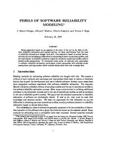
Fig.4 Parameter b

Mˆ ( N + p | N ) - M ( N + p ) M ( N + p)

Fig.5 Relative error Fig.1

h (k )

Table 1 and Table 2 show the estimation and prediction of cumulative number of software failures. We can find that the relative errors are very small. Fig.1 illustrates the effect of time series h (k ) . Fig.2 gives the curve of parameter q (k ) and its estimation and prediction, q (k ) denotes the changing of direction and speed. In this Figure, besides lacking testing data in the beginning of estimation, all estimations of q (k ) are less than 0.15. We can have the result that the trending of software reliability is increasing step by step. Fig.3 shows the observed, estimated and predicted result of time series nonlinear model M (k ) . In Fig.4, we get the curve of parameter b . In the processing of error removal, b is not a constant value and it changes continuously. We can see that this estimation accords with the characteristic of software testing error removal. Parameter b can show the speed and efficiency of error removal. In the beginning of test, the degressive speed of parameter b is very fast, it shows that the efficiency of error removal is very high and the software reliability increases rapidly. In the middle phase, b is stable relatively which indicates the efficiency of error removal is unchangeable. After

Fig.2 q (k ) , qˆ(k ) and qˆ( N + p | N )

Fig.3 M (k ) , Mˆ (k ) and Mˆ ( N + p | N )

4


stated periods, b increases and it shows that the efficiency of software error removal is lower and the growth of software reliability is slow down. In that new errors can be introduced into the software during the error removal process and the error numbers are more than that of removal, we must find out the reason and get a solution. At last, b stabilizes to 0.0014 and it shows that the efficiency of error removal has no change and software reliability is increasing steadily. Fig.5 illustrates the relative errors and shows good evaluation results of the new nonlinear model.

Fig.7

Software reliability index R

Table 4 Fuzzy evaluation of software reliability index

6 Software Reliability and Its Fuzzy Evaluation

R

( - ¥ ,1) [1,1.5) [1.5, 2) [2,2.5) [2.5,3) [3, + ¥ )

Software extremely Very lower higher low reliability low

From Fig.2, we can see that when q (k ) is closer to zero, the number of remaining errors is less and software reliability is higher. So the objective of software reliability can be designed

very extremely high high

Through Table 4, we can get more practical results than former evaluation. For example, one possible result of software reliability fuzzy evaluation is “software reliability is very high and can use soon” or “software reliability is general and the software should be tested further and improve reliability” and so on. In this example, R(108) = 2.8653 , the evaluation of software reliability is “very high” from Table 4.

R(k ) = -log(qˆ(k ))

(14) Simulation result is showed in Fig.6 and Fig.7. From the figures, we can see that software reliability rises on the whole trending. Strictly speaking, R (k ) is a fuzzy variable. So we can use fuzzy method to evaluate software reliability after analyzing and forecast reliability based on testing data. We compartmentalize some grades to R (k ) and use fuzzy variable to describe the software reliability. The results of fuzzy evaluation can be used to determine the covering range of the linguistic variables and confirm the fuzzy membership grade. Considering the fuzzy of variable R (k ) , we can establish relevant fuzzy linguistic variables and fuzzy rule to estimate software reliability as tabulated in Table 4.

7 Conclusion Although many SRGMs have been proposed since the first one appeared in 1972, no one model can suit all projects. While new projects arose, new SRGMs were created to suit them. It is difficult to propose a universal model to estimate and forecast software reliability. Through studying, we can find that testing data accord with the properties of time series. So we can apply proper time series model to evaluate software reliability. In the testing and modeling, we can find that nonlinear phenomenon exist in many situations and we can not neglect and deal with as linear model. This paper proposes a new method to establish software reliability. The new nonlinear forecasting model of software reliability has been proposed. The new model consider the disturb noise of observed data and have no need for strict hypothesis condition and the parameters are changing with time. All these accord with the characteristic of real projects. This method has demonstrated good results in terms of accumulative failures. The nonlinear modeling

Fig.6 Evaluation function

5


Reliability, R-28(3), August, 1979, pp. 206-211. [7] PK Kapur, S. Younes, Modelling an imperfect debugging pheonmenon in software reliability, Microelectronics and Reliability, 1996, vol.36, pp. 645-650. [8] Z. Jelinski and PB Moranda, Software Reliability Research, Statistical Computer Performance Evaluation, Academic, New York, 1972, pp. 465-485. [9] Amerit L Goel., Software reliability models: Assumptions,limitations and applicability, IEEE transaction on software engineering, 1985, SE11 (12), pp. 1411~1425. [10] Zhang, X.; Pham, H., An analysis of factors affecting software reliability, Journal of Systems and Software, 2000, pp. 43-56. [11] Wang ZL., Time series Analysis, Publishing House of Chinese Statistics, 2000. [12] Granger Clive WJ, Teräsvirta Timo, A simple nonlinear time series model with misleading linear properties, Economics Letters, 62 ,1999, pp. 161165. [13] Stephen HKan, Metrics and Models in Software Quality Engineering Second Edition, Publishing House of Electronics Industry, 2004. [14] Dengzili, Theory and Application of Optimal Filtering: Modern Time Series Analysis Method, Publishing House of Harbin Institute of Technology, 2000. [15] M. R. Lyu, Ed., Handbook of Software Reliability Engineering, McGraw Hill, 1996.

technique can be used for nonlinear and nonstationary processes of the data. Finally, we introduce fuzzy theory and unify the fuzziness and randomness to evaluate software reliability. The results of simulation example show that the new method presented in this paper is very useful to evaluate software reliability. References: [1] FL. Popentiu, D.N. Boros, Software Reliability Growth Supermodels, Microelectronics and Reliability, 1996, Vol 36, No. 4, pp. 485-491. [2] Takamasa Nara, Masahiro Nakata, Akihiro Ooishi, Software Reliability Growth AnalysisApplication of NHPP Models and Its Evaluation, IEEE Transactions on Reliability, HASE 1996, pp. 222-227. [3] Huang Xizi, Software Reliability、Security and Quality Assurance, Publishing House of Electronics Industry, 2002. [4] J.Musa, A.Jannino, and K.Okumoto, Software Reliability- Measurement, Prediction, Application, McGraw Hill, New York,1987. [5] J.D. Musa, A theory of software reliability and its application, IEEE Transactions on Software Engineering, SE-1(3), September, 1975, pp. 312327. [6] AL Goel, K. Okumoto, Time-dependent error detection rate model for software reliability and other performance measures, IEEE Transactions on

6