Architecture-Based Software Reliability Modeling - ftp.cs.toronto.edu

Architecture-Based Software Reliability Modeling Wen-Li Wang Dai Pan Mei-Hwa Chen Computer Science Department SUNY Albany (wlwang, dpan, mhc)@cs.albany.edu Abstract In this paper, we present an architecture-based approach for modeling software reliability. Our approach aims at modeling reliability on various software infrastructures and in any stage of software life cycles. To this end, we utilize characteristics of architectural styles to capture nonuniform behaviors of software embodying heterogeneous architecture. Furthermore, a state model that synthesizes all different architectural styles embedded in the system is developed, allowing the Markov-based reliability model to be employed. Our model can be applied to software with heterogeneous architecture, can facilitate the making of architecture design decision, and is suitable for use in the testing and maintenance phases during which software changes take place. To validate the model, we applied it to an industrial real-time component-based financial system and obtained significant promising results. It is expected that our model have great potential for use to improve software quality effectively. Keywords: Software Architecture, Architectural Style, Markov Model, and Reliability Estimation 1. INTRODUCTION Software systems have significant impact on the world. A failure operation of software can lead to economic loss and may even cause loss of human lives, thus proving its importance in our daily life. Therefore, unreliable software is not acceptable and should be identified in the early stage of software development. Software reliability is one of the key metrics for determining the quality of software. It is often defined as the probability of a failure-free operation of a computer program within a specified exposure time interval [33]. Over the past two decades, a number of studies have been conducted

1

for measuring reliability of given software. As a result, a number of analytical models [14, 33] have been introduced. Most of these analytical models focus on observing the behaviors of software, based on an operational profile. Measurements are made using the data collected over the observation period, regardless of the structure of the software. They are mainly applied during the late phase of the software development in order to determine if the software meets its reliability requirements. These models, which use statistical means, are difficult to apply if no sufficient test data is available or when changes are made to the software. Other approaches utilize Markov property and make use of the structure of software, which is typically applied to software with simple homogeneous architecture. However, modern software often embodies complex heterogeneous architecture to achieve multiple quality requirements, such as the use of a parallel architecture to increase performance and/or introduce a back-up component to provide fault tolerance. Moreover, vast growing component-based software that assembled using certain third party components requires adapting frequent component upgrade. Those with these infrastructures cannot be applied directly using the existing white-box Markov-based model. The aim of our model is to take heterogeneity of software architecture into account and allow it to be applied to various types of software infrastructures at an early stage of software development. Software architecture, which describes the structure of software at an abstract level [17, 34], consists of a set of components, connectors and configurations. Furthermore, a pattern that characterizes the configurations of components and connectors of software architectures is considered an architectural style [13, 15]. Many architectural styles have been identified [17, 36, 40] with new styles continuously emerging [32]. Thus, a practitioner can be faced with the challenge of selecting suitable styles and/or modeling configurations of selected styles for designing the architecture of a given software specification. In such a situation, a method or model to predict or evaluate the reliability of a heterogeneous software system can certainly provide a means through which designers can configure the architecture that best fits their quality

2

demands. Our previous studies [8, 41] suggest that it is possible to select an architectural style that can provide better performance and/or availability at the architecture design stage. In our approach, we utilize existing architectural styles that have well-defined characteristics to analyze architecture of the software system that has non-uniform behaviors in different portions of the system. We first identify the architectural styles in the system and develop a state machine for each style based on the behavior encapsulated. Next, the state machine that unifies the renderings of individual architectural styles in the system is formulated. With this unified state machine, we can further apply the Markov model to obtain reliability of the software using traditional approaches [11, 33]. Four architectural styles are used to demonstrate the development of the state machine. These styles include batch-sequential, parallel/pipe-filter, fault tolerance, and call-and-return architectural styles. We also describe how a variation of these styles can be incorporated using certain transformations. To validate our model, we conducted an experiment on an industrial realtime component-based financial system; the reliability measure obtained from the model was close to the observed value. Therefore, we believe that our model has great potential for use in heterogeneous software systems with the ability of being applied early in the design stage for aiding decision-making and late in the testing and maintenance phases for fast adjustment of reliability on software that has been changed. The scope of this paper is organized as follows: In Section 2 we give a brief overview of the Markov-based model and the foundations of our architecture-based software reliability model. The details of our style-based and then architecture-based models are described in Section 3 and 4, respectively. Section 5 presents a case study conducted on an industrial system to validate the model. Section 6 gives a brief overview of the related-work on software reliability measurements. Conclusions and future work are given in Section 7.

3

2. MODEL FOUNDATIONS Our architecture-based software reliability model utilizes discrete-time Markov chains to compute system reliability. In this section, we present the properties of discrete-time Markov model that serves as the foundations of our model. A discrete-time Markov chain consists of 1) A finite set of states S = {s1, ……., sn}, 2) A n × n stochastic matrix T = (Pij), where Pij is the transition probability that the system will move to state sj, given only that the system is in state si, and 3) A vector π 0 = (π 10 ,..., π n0 ) where π 0 denotes the probability that the system is initially in state si, i = 1,…,n. n

, where Pij ≥ 0, 1 ≤ i, j ≤ n, and ∑ Pij = 1, 1 ≤ i ≤ n j =1

In addition, a stochastic matrix is associated with the following two important properties that are crucial to our model [7]. 1) If T is a non-negative n × n stochastic matrix in the standard form as shown below, then ρ(M ) < 1 .  D1  0 T = M  0 B  1

L

0

D2 L

0

0 M

O

M

0

L Dr

B2

L Br

0  0 M  LLLL a standard form,  0 M 

where Di is an ni × ni irreducible state transition matrix associated with its ergodic equivalence class and M is a k × k square matrix and all the states corresponding to M are transient. Here, ρ(M ) is an eigenvalue of matrix M.

2) Let I be a k × k identity matrix. If M is a k × k matrix with ρ(M ) < 1 , then (I −M)−1 is nonsingular and (I − M ) = lim −1

k →∞

∞

k

∑M = ∑M . i

i =0

i

i =0

4

In [11], Cheung derived a reliability model following discrete-time Markov chains to model homogeneous software, in which common system structures such as branching and module-tomodule transitions were modeled. A system with k components will have k mapping states, where state si has component ci activated, 1≤i≤k. For generality, a system is considered only a single entry state s1 and a single exit state sk with π 1 0 = 1. With its simplicity of homogeneity, the entries of a k × k transition matrix M can be calculated as follows. Here, M(i,j) is the entry of ith row and jth column.  M (i , j ) = R i Pij , state s i reaches state s j and i ≠ k , for 1 ≤ i, j ≤ k …………………...…….. (1)   M (i, j ) = 0, otherwise

The system reliability is computed as R = (− 1)

k +1

Rk

E I −M

. Here, Ri is the reliability of

component ci. I is an k × k identity matrix and |I - M| is the determinant of matrix (I - M). |E| is the determinant of the remaining matrix excluding the last row and the first column of the matrix (I M). Although the homogeneity of Cheung’s model can be utilized to model component transitions and branching, it is insufficient to model some other structures and heterogeneous architectures. For example, a parallel architecture has multiple components running concurrently, a fault tolerant system has backup components compensating the failure of the others, or a calling component calls other components many times but executes only one time itself. Such structures can have multiple activities taking place simultaneously or require some specific actions based on the running situations. The combination of the different structures, becoming heterogeneous architectures, makes the use of this model even more challenging. To model such software, there is a need to construct a state model capable of addressing the heterogeneity. From [2], a state can be a set of circumstances or attributes characterizing a system at a given condition or activity. In our architecture-based reliability model, given that a condition is an

5

instance of a set of components from receiving the control to the release of control and a circumstance is an event that activates one of the components retaining the control. We define our state model as follows: -

A state is a set of circumstances characterizing a system at a given condition.

-

A transition is a passage from one state to another, whose transition probability is the probability of undergoing this transition.

Here, we also consider only a single entry state s1 and a single exit state sk with π 1 0 = 1. Note that multiple inputs and outputs can be modeled by introducing a super-initial state connecting to all the input states and a super-final state connecting from all the output states with individual transition probabilities. We want to construct a non-negative n × n stochastic matrix T as (2) without violating those two aforementioned properties.

S T=

S F s1 Lsk

F

1 0 0 1   B1 B2

k   1 M (1, j)  −  s1 Lsk 0 j =1   M 0 ,   ……………………………………...(2) M  , B = B = 1  0 2  k 0  1 − M (k −1, j)  + M   j =1  Rk  +   1 R − k  

∑

∑

Since matrix T is a stochastic matrix, each row sum of T is equal to 1. Two states S and F are the absorbing states, representing the successful output state and failure state, respectively. The transitions from S to S and F to F are equal to 1 because of absorbing states. M is a k × k matrix with only transient states, in which each row sum is less or equal to 1. The last row sum of M is equal to 0 because the exit state sk can only reach either the successful output state S, or the failure state F. B1 and B2 are k × 1 matrices. Since only the exit state sk can reach the successful output state S, all the entries of B1 are 0 except the final entry B1(k,0) equal to Rk+ , which is the

probability of the component(s) running reliably in state sk.. With the last row sum of M equal to 0, B2(k,0) is thus equal to 1-B1(k,0) and the other entries of B2 are equal to 1 minus the row sum of M in the same row. D1 = [1] and D2 = [1] are irreducible state transition matrices. So

6

T

is

in

standard

form

with ρ(M ) < 1 .

Therefore,

(I − M )−1

is

nonsingular,

and

∞

(I − M )−1 = ∑ M i . i =0

We can now adapt Cheung’s formula for computing system reliability as R = (− 1)

k +1

Rk+

E I −M

.

If only one component is activated in the exit state sk, then Rk+ = Rk ; otherwise, the computation of Rk+ relies on the system structures. We utilize architectural styles to realize the system structures and transform the architecture into a state model to derive the matrix M. Thus, the system reliability R can be calculated accordingly. The details are described in the next two sections. 3. STYLE-BASED RELIABILITY MODELING

Software architectural styles can be used to characterize software systems that share certain common properties, such as structure of organizations, constraints, and high-level semantics [15]. A number of architectural styles have been identified and used to facilitate the communications among developers and to better the understanding of software systems [17, 40]. The theme of our study is to evaluate the reliability of software based on its architecture. Software architectural styles allow us to comprehend complex system structures, especially, for those with heterogeneous architectures. Three attributes are required in our software reliability modeling. One is the system architecture, another is the set of component reliabilities, and the other is the set of transition probabilities for every two connecting components. The system architecture is classified into architectural styles to realize different interactions and intercommunications. The reliability of a component can be measured by traditional approaches [26, 30, 33] or the inter-component dependency approach proposed by Hamlet et al [22]. The transition probabilities are observed from the operational profile and are independent of component reliabilities. If component ci connects to n subsequent

7

components { c ki | 1 ≤ k ≤ n }, the transition probability Pij between components ci and c ij is equal n

to t (i, j )

∑ t (i, k ) . Here, t(i,j) is the total number of invocations or control transfers from k =1

component ci to c ij . In this section, we describe reliability modeling of software with single architectural style. For simplicity, the connector reliabilities will not be considered until the modeling of heterogeneous architecture in the next section. Four architectural styles are used to demonstrate how to model reliability of software with single architectural style. These styles include batch-sequential, parallel/pipe-filter, call-and-return, and fault tolerance styles. Other styles can be applied with some modifications. Throughout this paper, the following notations are used to describe our model. Ri represents the reliability of component ci, and Pij represents the probability of invocation or control transfer from component ci to one of its successor components cj. 3.1 Batch-sequential style

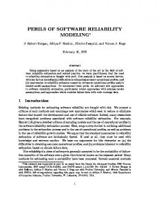
In the batch-sequential style, components are executed in a sequential order. In other words, only a single component is executed in any instance of time. Upon the completion of the execution, the control transfers from the executed component to one (and only one) of its successors. The selection of the succeeding component can be probabilistic (if more than one successors) or deterministic (if only one successor). This style can be modeled as shown in Figure 2(a), where c1, c2, … , ck are software components and a component, such as c2, can only transfer control to one of its branching subsequent components. Since only one component is executed at a time, the execution must be fully completed before the next component can proceed. Therefore, the state machine of a batchsequential style software can be modeled as follows: A state represents an execution of a component. A transition from one state to another takes place when the execution is completed,

8

and the control of the system transfers to the next component. The transformation from the architecture to a state model can be viewed as a mapping of a component to a state, shown in Figure 2(b), where s1, s2, …. , sk are the mapping states to components c1, c2, … , ck. (b) State Model

( a) Architecture

R1

c1

P12

R2

Rk

c2

ck

s1

R1 P12

s2

sk

Fig. 2: Batch-sequential style

The above architecture is composed of k components, so there will be k states. A k× k matrix M can be obtained the same as (1). 3.2 Parallel/Pipe-filter style

In a concurrent execution environment, components are commonly running simultaneously to improve performance. The parallel or pipe-filter styles are frequently used to model this type of systems. In these styles, components can be modeled to work simultaneously to fulfill a task. Each component works on a small partition or a subtask. The main difference between these two styles is that parallel computation is generally in multi-processors environment, whereas pipefilter style occurs commonly in a single processor, multi-processes environment. The state machine of a paralle/pipe-filter style software can be modeled as follows: If only one single component running, a state represents an execution of a component. Otherwise, we model the scenario of concurrent components by a state spanning the time from the beginning to the completion of the executions of these concurrent components. A transition from one state to another takes place when the execution is synchronized and completed, and the control of the system transfers to the next component. The transformation from the architecture to a state model can be viewed as a mapping of a single component to a state or multiple concurrent components to a state. In the dotted area of Figure 3(a), components c2 to ck-1 are running concurrently. They work on a portion of the output coming from component c2 and release the control to their common

9

subsequent component ck. Figure 3(b) is the state diagram of this architecture instance of the parallel/pipe-filter architectural style. The execution of component c1 is one single component running so is component ck. They are mapped to their individual states s1 and s3. The executions of components c2 to ck-1 are congregated into a state s2 representing multiple components running concurrently. ( a) Architecture

R1

P12

c1

c2

c3

(b) State Model

R2 P2 k

Rk

s1

ck

s2

R1 P12

s3

k −1

∏R P

l lk

l =2

c k −1

Fig. 3: Parallel or pipe-filter style

In Figure 3(a), there are k components in which k - 2 components are running concurrently into the same state; therefore, the total number of states is equal to 3. Because of the characteristics of parallel style, the transition probabilities from component c1 to components c2, c3, …., and ck-1, are all equal to P12. Therefore, the entry M(1,2), the transformed transition probability from state s1 to s2, is equal to R1P12. Entry M(2,3) means that all the components from c2 to ck-1 in state s2

perform successfully and finally reach state s3. Because component reliabilities and transition k −1

probabilities are independent of each other, therefore the value of M(2,3) is equal to

∏RP l

lk

,

l =2

which is the product of all the component reliabilities in this state and the transition probabilities from components c2, c3, …, and ck-1 to component ck, respectively. For the above architecture, a 3 × 3 matrix M is obtained as:  M (1, 2) = R1 P12 , s1 reaches s 2 k −1  Rl Pl 3 , c 2 to c k −1 running parallel in s 2 , for 1 ≤ i, j ≤ 3 ……………………….(3)  M ( 2,3) = l =2   M (i, j ) = 0, otherwise

∏

3.3 Fault Tolerance

The fault-tolerant architectural style consists of a set of components compensating for the failure of the primary component. When the primary component fails, the first backup component will

10

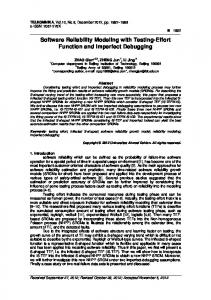
take over the responsibility and become the new primary component. If the new one fails as well, another backup component will take over. The implementation of these fault-tolerant components may involve using different algorithms and data structures to improve the system reliability. Therefore, the reliability of components in the same fault-tolerant set can be different from each other. In this style, components that compensate for the failure of each other are mapped into a state and the software will fail only when all the fault tolerant components fail. The state machine of a fault tolerant style software can be modeled as follows: If only one single component running, a state represents an execution of a component. Otherwise, we model the scenario of fault tolerant components by a state spanning the time from the beginning of the primary component to the completion of all the activated fault tolerant components. A transition from one state to another takes place when the execution is completed and the control of the system transfers to the next component. The transformation from the architecture to a state model can be viewed as a mapping of a single component to a state or multiple fault tolerant components to a state. Given the architecture displayed in Figure 4(a), those dotted components from c3 to ck-3 are modeled as backup components to the primary component c2. Inside the dotted rectangle shown in Figure 4(b), these components are congregated into the state s2 to represent multiple components running as fault tolerance. ( a) Architecture

P12

c1 R1

(b) State Model

c2

c3

P2( k − 2) P2( k −1)

s3

ck

c k −1 c k −3

s2

ck −2 s1

Rk

s5

R1 P12

s4

Rk −1

Fig. 4: Fault tolerance style

From Figure 4(a), assume that there are k components in which k - 4 components are running as fault tolerance; therefore, the total number of states is equal to 5. The concurrent characteristics of

11

fault tolerance style is similar to parallel style, where the transition probabilities from component c1 to components c2, c3, …., and ck-3, are all equal to P12. Thus, M(1,2) is equal to R1P12, the transformed transition probability between states s1 and s2. In general, all the backup components have the same transition probability as the primary component to its subsequent components. However, component c3 improves the reliability only when component c2 fails. Similarly, component c4 enhances the reliability only when both components c2 and c3 fail. So when we eliminate all possible unreliable conditions of the

  k −3  components, the left 1 −  (1 − Rl )  is the actual reliability. Therefore, the values of M(2,3)      l =2

∏

  k −3   k −3   and M(2,4) are equal to 1 −  (1 − Rl )  P23 and 1 −  (1 − Rl )  P24 , respectively.         l =2   l =2

∏

∏

For the fault tolerance architecture in Figure 4(a), a 5 × 5 matrix M can be constructed as follows: M (i, j ) = Ri Pij , s i is not fault tolerance and reaches s j  k −3   M (2, j ) = 1 −  1 − Rl )  Pij (     , for 1 ≤ i, j ≤ 5 ………….(4)     l =2  , c 2 to c k −3 are fault tolerant components in s 2 that reaches s j  M (i, j ) = 0, otherwise

∏

3.4 Call-and-return

In a call-and-return style, a calling component may request services provided by the called components. Before the services are fulfilled by the called components, the control remains on the calling component. After that, the calling component resumes the execution from where it left. Eventually, the component transfers its complete control authority to the next subsequent component. Therefore, the called components may be executed multiple times with only one time execution of the calling component. The state machine of a call-and-return style software can be modeled as follows: A state represents an execution of a component. A transition from one state to another takes place when the execution is completed and the control of the system transfers to the next

12

component, or the execution encounters a context switch and the control temporarily transfers to the called component. The transformation from the architecture to a state model can be viewed as a mapping of a component to a state. As shown in Figure 5(b), the state model is modeled by oneto-one mapping to the architecture of Figure 5(a), where state s1 is the calling state while s2 is the called state that provides services. During the execution, state s2 can be visited multiple times before state s1 gives control over to the final state s3. P12

(b) State Model

( a) Architecture

c1 R1 P13

c3

P12

c2

P21

R2

s1 R1 P12

s2 s3

R 2 P21

R3

Fig. 5: Call-and-return style

The entry M(1,3) is equal to R1P13, which is the reliability of client c1 multiplied by the transition probability from c1 to c3. Likewise, the entry M(2,1) can be computed as the reliability of server c2 multiplied by the transition probability from c2 to c1. The most important entry is M(1,2) which only considers the transition between s1 and s2 without considering the reliability of the client. This is because state s1 will be visited only once before entering state s3 regardless of how many times state s2 is visited. Therefore, the reliability of client c1 only needs to be considered when state s1 transits to state s3. For the architecture in Figure 5(a), the total number of states is therefore equal to 3. The 3 × 3 matrix M can be constructed as follows:  M (i, j ) = Ri Pij , s i reaches s j , where s j is not a called state  , for 1 ≤ i, j ≤ 3 …..………..….(5)  M (i, j ) = Pij , s i reaches s j , where s j is a called state  M (i, j ) = 0, otherwise 

Deterministic and Infinite Flow Problem:

In some cases the call-and-return style can be more complicated than the one described above, such as nested or transitive call where a caller is called by other component at the same time. In

13

this situation the control transfers among components can become infinite, as shown in Figure 6, and may face with the state explosion problem which differ from the case where cyclic loop is introduced in batch-sequential style, in which no state expansion is necessary. Furthermore, deterministic instead of probabilistic behaviors commonly exist in a system. For example, component A calls component B, when returns, A then calls component C. In this case, we cannot assign transition probabilities from A to B and A to C, which becomes probabilistic not deterministic. We brief our solution for this problem in this paper and refer the details of the algorithm to [41]. A

B

C

B

C

B

C

or D

E

or

D

or

E

D

E

F

Fig. 6: Infinite Control Transfers

To overcome the deterministic transition problem, the deterministic running sequence has been proven to have the same reliability measures as the batch-sequential style. Therefore, we can transform the architecture into batch-sequential style and utilize the method for batch-sequential style described in Section 3.1 to model the reliability. For the infinite control flow problem, the state model can suffer from infinite state expansion, which limits the utilization of Markov models. We introduce a transformation scheme to reduce infinite states into finite states. The key idea of this transformation scheme is to ensure that the state model covers all the control flow paths and the total number of executions of each component remains the same after the transformation. The transformation scheme requires the modifications on the component execution order. Based on the commutative law, ab is equal to ba if a and b are numbers. Because the entries of the transition matrix are numbers, as long as all

14

the control flow paths are covered and the total number of executions of each component has not been changed, the alter on the execution order will obtain the same reliability result. 4. ARCHITECTURE-BASED RELIABILITY MODELING

We have shown how to compute the reliability of a system based on a single architectural style in the previous section. For software architecture composed of heterogeneous styles, the reliability of a system can be modeled in four steps as follows. Assuming that the reliabilities of components and an operational profile are obtained and the transition probabilities have been computed. Step 1: Identify the architectural styles in a system, based on the design specification of a system. Step 2: Transform individual architectures of the identified architectural styles into state models. Step 3: Integrate these state models into a global state model of the system, based on the overall

architecture of a complete system.

Assuming that total x components are in software system G . After the architecture to state model transformations, we obtain a state set δ which consists of n states. Thus, we have G = { c τ | component c τ ∈ B U P U F U S U C , 1 ≤ τ ≤ x }

B : set of components in batch sequential style. P : set of components embedded in parallel style. F : set of components embedded in fault-tolerant style. S : set of called components in call-and-return style. C : set of calling components in call-and-return style.

where δ B : states mapped to the components in batch sequential style, δ B ={ s cτ | cτ ∈ B } δ P : states of u sets of parallel styles, where each state s p j consists of a set p j of parallel

components working together concurrently, δ P ={ s p j | cτ ∈ p j and p j ⊂ P , 0 ≤ j ≤ u }

15

δ F : states of v sets of fault-tolerant styles, where each state s f k consists of a set f k of

fault-tolerant components compensating for the failure of each other, δ F ={ s fk | cτ ∈ f k and f k ⊂ F , 0 ≤ k ≤ v } δ C : states of calling components in call-and-return style, δ C ={ s cτ | cτ ∈ C } δ S : states of called components in call-and-return style, δ S ={ s cτ | cτ ∈ S }

After the union of the different state sets δ = δ B U δ P U δ F U δC U δ S , we get δ = n . We then enumerate the index of each state Si from these n collected states, 1 ≤ i ≤ n . Step 4: Construct the transition Matrix M based on the global state model of the system and

compute the reliability of the system. We can consolidate formulas 2 to 5 to construct the k × k matrix M with total k states of a heterogeneous software architecture. In addition, the connector reliability Lij between components ci and cj can be taken into account and modeled into matrix M as shown below:      M (i , j ) =      

0 R i L ij Pij τ +q    R l L lj  P(τ +1) j   l =τ +1    a+r  1 −    P( a +1 ) j − 1 R L l lj    l a 1 = +    L ij Pij

∏

∏(

)

if s i can not reach s j , or i = k if s i ∉ δ P U δ F and s j ∉ δ S if s i ∈ δ P and c τ +1 to c τ + q are in s i if s i ∈ δ B and c a +1 to c a + r are in s i if s i calls s j , s j ∈ δ S

, where 1 ≤ i, j ≤ k . 5. A CASE STUDY

We conducted a case study to investigate the feasibility and limitations of the architecture-based reliability model on real systems. The empirical study was conducted on an industrial real time component-based system, which has been used by more than 100 companies and 4000 individual users over the past two years. This system provides a set of statistical models to help traders and fund managers analyze the stock market’s historical data and catch the future movement.

16

The system is composed of several sub-units including data unit, business rule unit, utility unit, and presentation unit. These units serve as the mathematical libraries and were implemented using C and C++. In this study, we focused on the data unit, which contains 54 classes, 13,846 lines of code, and 921 functions. It has a total of 15 components embedded with three architectural styles, batch-sequential, parallel, and client-server. The database components run concurrently with the evaluation components so that modeling and data retrieval can operate simultaneously. Two components, Calculator and Matrix, serve as server components to provide complex mathematics calculations for the client components. The other components are running in sequential manner with looping and branching conditions. To measure the system reliability, we use the test pool of the system provided by Quality Assurance team and run 13,596 test inputs. Among these, we observe 121 failures and obtained system reliability 0.9911. To apply our model, the transition probabilities between components were collected from those 13,596 test inputs. For the transition probability between two components ci and cj, the value is calculated as the number of transitions from ci to cj over the total number of transitions from ci to all its succeeding components. To measure the component reliability, for each component we use data recorded by QA team during unit testing and compute the number of successful execution without crash over the total number of executions. The number of testing inputs for each component can be different depending on the component complexity. We constructed the state machine of the system using the methodologies described in Section 3 and 4 and then utilized Markov model to compute the system reliability using formula (3). The system reliability computed from the model is 0.994001. We notice approximately 0.003 difference between the reliability observed and the reliability computed from the model. The difference is caused by the probabilistic characteristics of Markov model without taking into account the deterministic behaviors such as component ci always first calls or transits to cj and

17

then calls or transits to ck.. To tackle this situation, more efforts are required to refine the state model, which is beyond the scope of this paper. 6. RELATED WORK

Software Reliability Growth Models (SRGMs) employ test history to predict Mean Time To Failure of the software [14, 33]. Using a black box approach, these models require re-testing the whole software if a change or an update occurs to the structure. Today, software components can easily plug-and-play and upgrade, which ease the software development but hinder the use of SRGMs due to repeated testing efforts. A number of studies adopt Markov models to measure the reliability of modular software. Cheung [11] proposed a user-oriented reliability model to measure the reliability of service that a system provides to a user community. A discrete Markov model was formulated based on the knowledge of individual module reliability and inter-module transition probabilities. In Littlewood’s reliability model [29], a modular program is treated as transfers of control between modules following a semi-Markov process. Each module is failure-prone, and the different failure processes are assumed to be Poisson. Laprie et. al [27] evaluate the reliability of multi-component systems by introducing a knowledge-action transformation (KAT) model, which accounts for reliability growth phenomena, and enables estimation and prediction of the reliability of multicomponent systems. These models are limited to model sophisticated structures and heterogeneous architectures, but can handle homogeneous software with common sequential and branching transitions. In addition to analytic models, experiments and simulations were also developed to predict and measure software reliability. Krishnamurthy and Mathur [24] conducted an experiment to evaluate a method, Component Based Reliability Estimation (CBRE), to estimate software reliability using software components. CBRE involves computing path reliability estimates based on the sequence of components executed for each test input and the system reliability is the average over all test runs. Gokhale et al [19] proposed a discrete-event simulation to capture a

18

detailed system structure and to study the influence of separate factors in a combined fashion on dependability measures. Li et al [28] presented a methodology and accompanying toolset, W2S, for generating a simulator from a semi-formal architecture description, which allows an analysis of the system's reliability based on it’s simulated behavior and performance. Gokhale et al [21] predicted architecture-based software reliability using a testing-based approach, which parameterized the analytic model of the software using measurements obtained from the regression test suite, and coverage measurements. The above approaches are able to model certain system structures, but are usually expensive and time-consuming especially when applying to structure changes, and the application domains can be limited.

7. CONCLUSIONS

We present an architecture-based approach for modeling software reliability, which can be used to measure reliability on various software infrastructures in early phase of software development. By means of architectural styles, software with heterogeneous architectures that behaves nonuniformly across different portions of the system can be analyzed and modeled using a state machine. The high-level architecture-based software reliability modeling facilitates quality assessment at an early stage of the software life cycle, thus benefiting decision-making on software architecture design. The architecture-based reliability modeling is a top-down approach, in which software is first examined based on the design requirements and classified into different architectural styles. With the study of the reliability modeling of each individual architectural style, the style-based reliability models can be used as the building blocks of an architecture-based reliability model for measuring overall system reliability. This approach takes software structures into account and does not rely on test data; therefore, it can be applied to the architecture design phase to guide the decisions of the selections of architectural styles, components, and configurations. Moreover, during the testing and maintenance phases, when a component is modified or a new component is

19

added to the system, the model can re-compute the reliability of the modified system without a complete re-testing. Our empirical study on the real system suggests its great potential for use in modern software infrastructures. REFERENCES

1. Abowd G., Bass L., Clements P., Kazman R., Northrop L., and Zaremski A., 1997. Recommended Best Industrial Practice for Software Architecture Evaluation, Technical Report CMU/SEI96TR 025 and ESCTR96025, January. 2. Agnes M., 2000. Webster’s New World Colledge Dictionary 4th Edition, Macmillan, USA, pp1399. 3. Allen R. and Garlan D., 1994. Formal Connectors, Technical Report CMUCS94115, Carnegie Mellon University. 4. Allen R. and Garlan D., 1994. Formalizing Architectural Connection, In Proceedings of the Sixteenth International Conference on Software Engineering, Sorrento, Italy, May. 5. Allen R. and Garlen D., 1992. Towards Formalized Software Architectures, CMU-CS-92163, July. 6. Bass L., Clements P., and Kazman R., 1998. Software Architecture in Practice, Addison Wesley Longman, Inc. 7. Berman A. and Plemmons R. J., 1979. Nonnegative Matrices in the Mathematical Sciences, Academic Press Inc., New York. 8. Chen M. H., Tang M. H., and Wang W. L., 1998. Effect of Software Architecture Configuration on the Reliability and Performance Estimation, In Proceedings of the 1998 IEEE Workshop on Application Specific Software Engineering and Technology, March. 9. Chen M. H., Lyu M. R., Rego V. J., Mathur A. P. and Wong E. W., 2001. Effect of Code Coverage on Software Reliability Measurement, In IEEE Transactions on Reliability 10. Chen M. H., Garg P., Mathur A. P. and Rego V. J., 1995. Investigating Coverage-Reliability Relationship and Sensitivity of Reliability Estimates to Errors in the Operational Profile, In

20

Computer Science and Informatics Journal - Special Issue on Software Engineering, 25(3):4, pp165-170, September. 11. Cheung R. C., 1980. A User-Oriented Software Reliability Model, IEEE Transactions On Software Engineering, 6(2):118, pp118-125, March. 12. Clements P. C., 1996. Coming Attractions in Software Architecture, Technical Report CMU/SEI96 TR008 and ESCTR96008, Carnegie Mellon University, Software Engineering Institute, January. 13. Dutton G. and Sims D., 1994. Patterns in OO Design And Code Could Improve Reuse, IEEE Software, 11(3):101, May. 14. Farr W., 1996. Software Reliability Modeling Survey, In M. R. Lyu editor, Handbook of Software Reliability Engineering, McGraw-Hill Publishing Company and IEEE Computer Society Press, New York, pp71-117. 15. Garlan D., 1995. What Is Style?, In Proceedings of Dagshtul Workshop on Software Architecture, February. 16. Garlan D., Allen R., and Ockerbloom J., 1994. Exploiting Style in Architectural Design Environments, In Proceedings of SIGSOFT'94: Foundations of Software Engineering. ACM Press, December. 17. Garlan D. and Shaw M., 1993. An Introduction to Software Architecture, In V. Ambriola and G. Tortora, editors, Advances in Software Engineering and Knowledge Engineering, volume 1. World Scientific Publishing Company. 18. Goel A. L. and Okumoto K., 1979. A Markovian Model for Reliability and Other Performance Measures of Software Systems, National Computer Conference. 19. Gokhale S. S., Lyu M. R., and Trivedi K. S., 1998. Reliability Simulation of ComponentBased Software Systems, In Proceedings of International Symposium on Software Reliability Engineering, pp192-201. 20. Gokhale S. S., Lyu M. R., and Trivedi K. S., 1998. Software Reliability Analysis

21

Incorporating Fault Detection and Debugging Activities, In Proceedings of International Symposium on Software Reliability Engineering, pp202-211. 21. Gokhale S. S., Wong W. E., Trivedi K. S., and Horgan J. R., 1998. An Analytical Approach to Architecturebased Software Reliability Prediction, In Proceedings of IEEE International Computer Performance and Dependability Symposium (IPDS), September. 22. Hamlet D., Mason D., and Woit D., 2001. Theory of Software Reliability Based on Components, 23rd International Conference on Software Engineering, May. 23. Kazman R., Abowd G., L. Bass and Clements P., 1996. Scenario-Based Analysis of Software Architecture, IEEE Software, November. 24. Krishnamurthy S. and Mathur A. P., 1997. On the Estimation of Reliability of a Software System Using Reliabilities of its Components, In Proceedings of Eighth International Symposium on Software Reliability Engineering, pp 146-155. 25. Lapri J-C., 1995. Dependability of Computer Systems: Concepts, Limits, Improvements, International Symposium on Software Reliability Engineering. 26. Laprie J-C. and Kanoun K., 1996. Software reliability and system reliability, Handbook of Software Reliability Engineering, pp 27-70, McGraw-Hill, New York. 27. Laprie J-C. and Kanoun K., et al., 1991. The KAT Approach to the Modeling and Evaluation of Reliability and Availability Growth, IEEE Transactions on Software Engineering, SE17(4):370-382. 28. Li J. J., Micallef J., and Horgan J. R., 1997. Automatic Simulation to Predict Software Architecture Reliability, In Proceedings of Eighth International Symposium on Software Reliability Engineering, pages 168-179. 29. Littlewood B., 1975. A Reliability Model for Systems with Markov Structure, Applied Statistics, 24(2):172. 30. Littlewood B., 1979. Software Reliability Model for Modular Program Structure, IEEE Transactions on Reliability, Vol. R-28, No. 3, August.

22

31. Lopez-Benitez N., 1994. Dependability Modeling and Analysis of Distributed Programs, IEEE Transactions on Software Engineering, Vol. 28, No. 5, May. 32. Medvidovic N., Oreizy P., and Taylor R. N., 1997. Reuse of Offtheshelf Components in C2 style Archtiectures, In Proceedings of 19th International Conference on Software Engineering, May. 33. Musa J., Iannino A., and Okumoto K., 1987. Software Reliability: Measurement, Prediction, Application, McGraw-Hill, New York. 34. Perry D. E. and Wolf A. L., 1992. Foundations for the Study of Software Architecture, ACM SIGSOFT Software Eng. Notes, 17(4):40-52, October. 35. Shaw M., et al., 1995. Abstractions for Software Architecture and Tools to Support Them. IEEE Transactions on software Engineering, April. 36. Shaw M., 1991. Heterogeneous Design Idioms for Software Architecture. In Proceedings of Sixth International Workshop on Software Specification and Design, IEEE, pp.158-165, October. 37. Shaw M. and Garlan D., 1994. Characteristics of Higher-level Languages for Software Architecture, Technical Report CMUCS94210, Carnegie Mellon University, December. 38. Shaw M. and Garlan D., 1996. Software Architecture: Perspectives on an Emerging Discipline, Prentice Hall. 39. Taylor R. Medvidovic N., N., Anderson K. M., Whitehead Jr. E. J., Robbins J. E., Nies K. A.,

Oreizy P., and Dubrow D. L., 1996. A Component and Message-based Architectural Style for GUI Software, IEEE Transactions on Software Engineering, June. 40. Tracz W., 1995. DSSA frequently asked questions (FAQ), ACM Software Engineering Notes, 19(2):52--56, June. 41. Wang W. L., and Chen M. H., 2001. Deterministic Software and Infinite Control Flow Modeling, SUNYA Technical Report TR11152001, November. 42. Wang W. L., Tang M. H., and Chen M. H., 1999. Software Architecture Analysis – A Case

23

Study, 23rd IEEE International Computer Software & Applications Conference. 43. Wang W. L., Wu Y. and Chen M. H., 1999. An Architecture-Based Software Reliability Model, In Proceedings of Pacific Rim International Symposium on Dependable Computing.

24