software testing and results comparison - ISPRS Archives

The International Archives of the Photogrammetry, Remote Sensing and Spatial Information Sciences, Volume XLII-2, 2018 ISPRS TC II Mid-term Symposium “Towards Photogrammetry 2020”, 4–7 June 2018, Riva del Garda, Italy

4D-SFM PHOTOGRAMMETRY FOR MONITORING SEDIMENT DYNAMICS IN A DEBRIS-FLOW CATCHMENT: SOFTWARE TESTING AND RESULTS COMPARISON S. Cucchiaroa,b , E. Masetc,∗, A. Fusielloc and F. Cazorzia a

b

DI4A – University of Udine, Via delle Scienze, 206 – Udine, Italy (sara.cucchiaro, federico.cazorzi)@uniud.it Department of Life Sciences – University of Trieste, Via E. Weiss, 2 – Trieste, Italy c DPIA – University of Udine, Via delle Scienze, 206 – Udine, Italy [email protected], [email protected] Commission II, WG II/10

KEY WORDS: 4D-SfM Photogrammetry, Sediment dynamics monitoring, Software comparison, Debris flow hazard

ABSTRACT: In recent years, the combination of Structure-from-Motion (SfM) algorithms and UAV-based aerial images has revolutionised 3D topographic surveys for natural environment monitoring, offering low-cost, fast and high quality data acquisition and processing. A continuous monitoring of the morphological changes through multi-temporal (4D) SfM surveys allows, e.g., to analyse the torrent dynamic also in complex topography environment like debris-flow catchments, provided that appropriate tools and procedures are employed in the data processing steps. In this work we test two different software packages (3DF Zephyr Aerial and Agisoft Photoscan) on a dataset composed of both UAV and terrestrial images acquired on a debris-flow reach (Moscardo torrent - North-eastern Italian Alps). Unlike other papers in the literature, we evaluate the results not only on the raw point clouds generated by the Structure-fromMotion and Multi-View Stereo algorithms, but also on the Digital Terrain Models (DTMs) created after post-processing. Outcomes show differences between the DTMs that can be considered irrelevant for the geomorphological phenomena under analysis. This study confirms that SfM photogrammetry can be a valuable tool for monitoring sediment dynamics, but accurate point cloud post-processing is required to reliably localize geomorphological changes.

1. INTRODUCTION Geomorphic processes such as debris flows are one of the main sources of risk for human lives and infrastructures in mountain catchments. Several countermeasures can be taken to mitigate their effects and, among all hydraulic engineering structures, check dams are the most common technique to manage debris flow hazard (Hübl et al., 2005, Piton et al., 2017). These control works significantly affect sediment dynamics and a continuous monitoring of the morphological evolution is therefore required to improve management strategies and torrent control planning (Victoriano et al., 2018). The acquisition of repeated topographic surveys lets not only to characterize debris flows in terms of their geomorphic activity, but also to infer the sediment dynamics at multiple temporal and spatial scales (4D) and their link to torrent control works. Being low-cost, automatic and easy to use, Structure-from-Motion (SfM) photogrammetry represents a powerful alternative to laser scanning technique for acquiring high-resolution topography in a variety of environments (Westoby et al., 2012, James and Robson, 2012, Smith and Vericat, 2015, Carrivick et al., 2016), allowing also to increase the frequency of the surveys. Moreover, the possibility of integrating images acquired from the ground and by an Unmanned Aerial Vehicle (UAV), makes SfM and Multi-View Stereo (MVS) methodologies ideal tools to obtain a complete reconstruction of the topographic surface, even in the presence of steep slopes and areas characterized by limited accessibility as in debris flow catchments (Bemis et al., 2014). ∗ Corresponding

author

In the last years, many software packages have been developed to combine computer vision algorithms and photogrammetry principles in order to obtain accurate 3D reconstructions in an automatic way, without user interaction (Carrivick et al., 2016). Since this technique requires relatively little training and has a high level of automation, the majority of end-users consider the software as a black-box and they are often unaware of the accuracy and reliability of the obtained 3D model (Micheletti et al., 2015b, Smith et al., 2016). Many papers that provide an evaluation of the most popular commercial software solutions can be found in the literature (Nikolov and Madsen, 2016, Remondino et al., 2017) but they usually assess the accuracy on the point cloud generated by the SfM-MVS process (Aicardi et al., 2016). Instead, when monitoring geomorphological processes such as sediment dynamics, the point cloud represents only the initial step of the workflow that leads to create the Digital Terrain Model (DTM), a fundamental tool to study topography evolution. Indeed, DTMs derived from different surveys can be subsequently compared, i.e., the old DTM is subtracted to the new one (DTM of Difference, DoD) to identify morphological changes over time (Wheaton et al., 2010, Cavalli et al., 2017, Vericat et al., 2017). For these reasons, in this work we test two different software tools (3DF Zephyr Aerial v. 3.503 and Agisoft Photoscan v. 1.2.0) and evaluate the results not only on the raw point cloud, but also on the DTM obtained after post-processing. The paper is organized as follows. Section 2 describes in detail the image processing steps and the subsequent post-processing of the point clouds, which leads to the creation of the DTMs. In Sec. 3 the comparison between the results obtained by the two software packages is reported, focusing on the derived DoDs. Fi-

This contribution has been peer-reviewed. https://doi.org/10.5194/isprs-archives-XLII-2-281-2018 | © Authors 2018. CC BY 4.0 License.

281


nally, Sec. 4 draws the conclusions. 222 images Terrestrial + UAV Sony Alpha 5000 20 Mpx, f: 16mm

2. TESTS AND ANALYSES

222 images Terrestrial + UAV Sony Alpha 5000 20 Mpx, f: 16mm

I. Data acquisition

PS

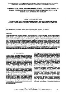
The following paragraphs describe in detail the image processing procedure and the dense point cloud post-processing steps carried out to compare 3DF Zephyr and Photoscan products. Figure 1 shows the complete workflow applied in this study (an exhaustive description of the post-processing phases can be found in (Cucchiaro et al., 2018b)). 2.1

Agisoft Lens

3DF Lapyx

III. Sparse point cloud

# oriented images: 222 computing time: 3h 45’ # 3D pts 241,917

RMSE CP (cm) X= 2.4 Y= 2.9 Z= 4.7

IV. Alignment error analysis

RMSE CP (cm) X= 2.0 Y= 1.9 Z= 5.9

pts/m2: 14219 computing time: 4h

V. Dense point cloud

This study was carried out in the Moscardo Torrent, a debrisflow creek in the Eastern Italian Alps (Fig. 2a) whose catchment drains an area of 4.1 km2 . This catchment is characterized by steep slopes prone to rockfalls and shallow landslides, which supply large amounts of debris to the channels (Marchi et al., 2002, Blasone et al., 2014). In order to mitigate the natural hazard related to debris flows, two new concrete check dams were recently built in the upper part of the basin, with the aim of retaining sediment transported by debris flows and stabilizing the banks side of the reach (more details regarding the effects of torrent control works in the Moscardo catchment can be found in (Cucchiaro et al., 2018a)).

Filtering: 13743 pts/m2 Decimation: 395 pts/m2

The effects of check dams on sediment dynamic have been investigated by means of multi-temporal SfM (4D-SfM) surveys after debris flow events in an area of approximately 3700 m2 . In particular, the performance evaluation of the two commercial packages previously mentioned was carried out on a dataset of 222 images acquired on May, 2017.

For the aerial survey of the area, the camera was mounted on a professional octorotor UAV (Neutech Airvision NT-4C, Fig. 3) and the flight was performed at an altitude of 20 m, resulting in a mean Ground Sample Distance (GSD) of 6 mm. For the groundbased survey, the photographs were taken maintaining an average depth distance from the object and a mean baseline between adjacent camera positions of around 3 m. Moreover, a total of 27 markers were located on stable areas (Fig. 2b). As suggested in (Piermattei et al., 2015), they were uniformly distributed, not aligned or clustered, in order to improve the quality of the final model and to mitigate systematic errors (James and Robson, 2012). The markers coordinates were measured by means of a Leica 1200 L1+L2 GPS system in Relative Stop&Go mode to increase accuracy using RINEX data of the nearby permanent station (Zouf Plan, 4 km away). The post-processing step allowed to reach a planimetric positional accuracy ranging from 0.01 m to 0.02 m and vertical uncertainties between 0.02 and 0.04 m.

II. Camera calibration

# oriented images: 222 computing time: 3h 48’ # 3D pts: 1,581,701

Data acquisition

For this study, an integrated approach combining terrestrial and aerial images (both collected with a Sony Alpha 5000 compact digital camera - 20 Mpixels APS-C CMOS sensor, focal length 16 mm) has been designed to overcome individual limitations of the two platforms. Aerial images, in fact, allow to cover large areas in short time but a nadiral image acquisition causes poor representation of steep terrain and vertical surfaces (Loye et al., 2016). Terrestrial images, instead, can provide a more accurate representation of complex surfaces but cover small areas and can be unreliable on relatively flat terrain (Piermattei et al., 2016).

3DFZ

VI. Post processing

pts/m2: 12634 computing time: 1h 52’

Filtering: 12192 pts/m2 Decimation: 395 pts/m2

Resolution: 0.2 m

VII. DTM realization

Resolution: 0.2 m

SD M3C2 distance to reference cloud in stable areas: 0.03 m

VIII. Uncertainty analysis

SD M3C2 distance to reference cloud in stable areas: 0.03 m

IX. DoD generation

Figure 1. Workflow applied for image processing and point cloud post-processing, together with a comparison of the results obtained through 3DF Zephyr (3DFZ) and Photoscan (PS). 2.2

Image processing

In order to equally compare the computing time of 3DF Zephyr (3DFZ) and Agisoft Photoscan (PS), the image dataset was processed with the same computer (Intel Core i7-6950x CPU @ 3.00Ghz and 128GB RAM, 3xNVIDIA GeForce GTX 970). Among the 27 markers, a subset of 14 points were used as GCPs during the Bundle Block Adjustment phase, whereas 13 points were employed as Check Points (CPs) for the accuracy evaluation (Fig. 2b). The image coordinates of the points were measured just once in PS and then imported and used in 3DFZ. A preliminary calibration of the camera (Fig. 1, blocks II) was carried out using the calibration modules of the two software (3DFZ Lapyx for 3DF Zephyr and Agisoft Lens for Photoscan). Furthermore, for the SfM and MVS phases the most similar settings were selected, adopting the same image resolution in the tie point extraction and dense image matching phases for both software packages. A comparison of the results of the SfM step is reported in Figure 1, blocks III and IV. Please note that both 3DFZ and PS oriented all the images and no problems were found in the simultaneous alignment of terrestrial and aerial photos. Studies in the literature that apply SfM for geomorphological change detection, instead, process separately aerial and terrestrial images (Eltner et al., 2016), fusing in a subsequent step the obtained point


282


Figure 2. (a) The Moscardo catchment and the study area location. (b) GCPs and CPs distribution in the study area.

Figure 3. The octorotor UAV used for the surveys. clouds (Stöcker et al., 2015). However, data fusion in the SfM process avoids further errors and misalignments that can arise when merging different point clouds. In order to determine the alignment accuracy, the RMSE (Root Mean Square Error) on n = 13 CPs was computed along the x direction as: v u n u1 X RMSEx =t · (XSfMi − XGPSi )2 (1) n i=1 where XSfM indicates the coordinate estimated from the SfM process, whereas XGPS refers to the CP coordinate measured with GPS technique (Remondino et al., 2017). Analogously, the RMSE was calculated on the y and z directions, and the 3D RMSE was estimated as: q RMSE3D = RMSE2x + RMSE2y + RMSE2z (2)

Figure 4. Detail of boulders reconstructed in the dense point clouds by 3DFZ (a) and PS (b). tool computes the local distance between two point clouds along the normal surface direction which tracks 3D variations in surface orientation. The results will be discussed in detail in Sec. 3. 2.3

Very similar accuracy in object space was achieved: the 3D RMSE on the CPs is 6.5 cm for 3DFZ and 6.0 cm for PS. The MVS algorithm (Fig. 1, block V) of both software packages generated high-density point clouds (47,544,425 points for 3DFZ and 53,506,387 points for PS) that perfectly reconstruct even small features of the scene. An example of the obtained high level of detail is illustrated in Fig. 4, where it is possible to notice that even small boulders are accurately reconstructed. The M3C2 (Multiscale Model to Model Cloud Comparison) tool (Lague et al., 2013) of CloudCompare software (Omnia Version: 2.9.1) was used to quantitatively evaluate the differences between the created dense point clouds (Cook, 2017). Specifically, the M3C2

Dense cloud post-processing

The cloud-to-cloud quantitative assessment is not sufficient to determine how the differences found between the point clouds, created by 3DF Zephyr and Photoscan, can affect subsequent analyses, e.g., the amount of debris mobilized and the estimate of erosional and depositional processes in time. Therefore, further evaluations were carried out on the DTMs generated from the dense point clouds through post-processing (Fig. 1 block VI). The point-cloud post-processing was performed by means of the CloudCompare software to reduce noise and erroneous points. A manual filtering was initially performed, followed by the the SOR filter (Statistical Outlier Removal filter) tool, which removes the outlier points by first computing the average distance of each


283


point to its neighbors and then rejecting the points that are farther than the average distance plus a number of times the standard deviation. Since the goal of this study is also to compare the 3DFZ and PS products with respect to a subsequent survey performed in July 2017 in order to asses geomorphological changes, the registration of the 3DFZ and PS point clouds to the July 2017 one was carried out. This step is needed when working with multitemporal data (Eltner et al., 2016, Williams et al., 2018): error on the GPS measures (the GCPs used for the georeferencing process are re-surveyed every time since they could have moved) and on the manual identification of markers on the images could produce inaccurate georeferencing and could lead to unreal shift or rotation between multi-temporal 3D models (Micheletti et al., 2015a, Carrivick et al., 2016).Therefore, the Iterative Closest Point (ICP) algorithm (Zhang, 1994) of CloudCompare was used to automatically co-register point clouds of May 2017, adopting as reference one the 3D model of July 2017. In particular, the ICP algorithm was performed on a subset of the point clouds, corresponding to stable areas (e.g. the check dams structures), and then the obtained rigid transformation was applied to the whole original point clouds. Furthermore, since a direct interpolation of extremely dense point cloud (> 104 points/m2 ) into a coarser resolution terrain model can be an unfeasible computational task, the raw point clouds were decimated through the geostatistical Topography Point Cloud Analysis Toolkit (ToPCAT), implemented in the Geomorphic Change Detection software for Esri ArcGIS, (Wheaton et al., 2010). ToPCAT is an efficient decimation procedure that decompose the point cloud into a set of non-overlapping grid-cells and calculate statistics for the observations in each grid (Vericat et al., 2014). The minimum elevation within each grid-cell is considered the ground elevation (Brasington et al., 2012) and is used to create a TIN (Triangular Irregular Network), a surface representation that is computationally efficient in complex fluvial geomorphology (Brasington et al., 2000, Heritage et al., 2009). The Esri ArcGis Natural Neighbors interpolator was then used to obtain two DTMs with a resolution of 0.2 m (Fig. 1 block VII). 2.4

DTM of Difference (DoD) generation

Finally, both DTMs derived from 3DFZ and PS point clouds were compared with the one realized from the survey of July 2017, creating in this way two DoDs (Fig. 1 block IX) in order to determine the spatial patterns and associated volumes of morphological change (Cavalli et al., 2017). In DoDs generation a fundamental aspect to consider is the uncertainty estimation of the used DTM (Fig. 1 block VIII) (Lane and Chandler, 2003, Wheaton et al., 2010, Vericat et al., 2017). Several factors can indeed introduce errors in DTM, including survey point quality, sampling technique, surface characteristics (e.g., wet surfaces produce high errors in MVS reconstruction due to the water high reflection), topography complexity and interpolation methods (Milan et al., 2011, Passalacqua et al., 2015). The most commonly adopted procedure for managing DTM uncertainties involves specifying a minimum level of detection threshold (minLoD) to distinguish real surface changes from the inherent noise (Brasington et al., 2003, Wheaton et al., 2010, Marteau et al., 2017). This threshold is chosen according to the error estimate of each DTM and the Confidence Interval (CI) considered. In this study, the uncertainty level of each model was assessed through the M3C2 tool of CloudCompare, calculating the cloud-

to-cloud distance between each May 2017 post-processed cloud (generated by Photoscan and 3DF Zephyr) and the July 2017 one. The computation was carried out in wide stable surfaces (e.g., the structure of check dams or stone and concrete banks), where no topographic changes over time were expected (Fig. 1 block VIII). More specifically, the standard deviation of this distance was used as an indicator of the uncertainty related to the pair of point clouds under analysis and consequently it was assumed as the uncertainty (εDTM ) affecting the corresponding DTMs. Therefore, the minimum Level of Detection (minLoD) was calculated as in (Brasington et al., 2003): q minLoD = t · (εDTM1 )2 + (εDTM2 )2 (3) where εDTM1 and εDTM2 are the errors estimated for the most recent and the oldest DTM, respectively, and t is the t-score (for a conservative approach a value of t = 1.96 was used, corresponding to a confidential interval of 0.95). In this case, εDTM = 3 cm was assumed as the uncertainty value for all the DTMs. When analysing the DoDs, discrepancies above minLoD were regarded as real changes, while the differences below this threshold were considered uncertain and not used in the final volume computation. The last analysis concerns the estimation of erosion and deposition volumes, that can be easily performed thanks to the change in elevation provided by the DoDs for each grid cell and knowing the cell size.

3. RESULTS AND DISCUSSION The employed image processing procedure shows that similar dense point clouds in terms of density are generated from both 3DFZ and PS software (12,634 points/m2 for 3DFZ and 14,219 points/m2 for PS). The high density derives also from the integrated approach of ground-based images and aerial acquisition, that allows to obtain SfM-MVS models without missing data and fewer deformation errors. Moreover, the M3C2 distance analysis, as shown in Fig. 5, reveals that the absolute difference between the two point clouds is on average 4.2 cm, with a standard deviation of 3.4 cm. These discrepancies are minimal, with the exception of some regions on the border of the study area and the red zone in Fig. 5 (in the middle of the study area, upstream the check dams). The images acquired in these areas suffer from poor overlap, caused also by the fact that the UAV took off and landed in this specific zone between two consecutive phases of the flight. This could have influenced the reliability of the solution computed by the two software for these specific images. Please note also that the flight was carried out in manual fly mode, due to difficult environmental conditions (including wind, low GPS signal, high vegetation and complex topography), resulting in a non optimal camera network geometry (Fig. 6). The difference between PS and 3DFZ dense clouds becomes insignificant after the post-processing that leads to DTMs and DoDs generation. Indeed, the resulting thresholded DoDs (with a minLoD around 8 cm, Figures 7 and 8) highlight that the post processing of the raw point clouds smoothed the small discrepancies between the output of the two software packages and the final products are almost identical. Further evidence of the equivalence between the two DTMs obtained from 3DFZ and PS is given by the deposition, erosion and net change volumes calculated from the DoDs, shown in Table 1. Note that the volume uncertainties


284


Figure 5. Distance map between 3DFZ and PS dense point clouds of May 2017 survey (best viewed in color).

Figure 6. Camera network geometry determined by 3DFZ. The blue pyramids represent the camera viewpoints, whereas the red circles are the GCPs employed in the Bundle Adjustment phase.

DoD

Erosion [m3 ]

Deposition [m3 ]

Net volume difference [m3 ]

July 2017- May 2017 (3DFZ)

55 ± 13

776 ± 99

720 ± 100

July 2017- May 2017 (PS)

54 ± 13

768 ± 98

713 ± 99

May 2017 (3DFZ) - May 2017 (3DFZ)

0.50 ± 0

0.73 ± 0.02

0.23 ± 0.02

Table 1. Total volume of erosion and deposition and net volume change for the computed DoDs.


285


Figure 7. DoD July 2017-May 2017 (dataset processed by 3DF Zephyr).

Figure 8. DoD July 2017-May 2017 (dataset processed by Photoscan).


286


(±) are estimated on the basis of the minLoD. The volume differences between the DoDs of 3DFZ (Fig. 7) and PS (Fig. 8) are very low (around 1 m3 for erosion process, 8 m3 for deposition volumes and 7 m3 in terms of net changes). This minimal dissimilarity is also confirmed by the thresholded DoD between 3DFZ and PS DTMs, where the volume difference is below 1 m3 in terms of erosion, deposition and net volume. The higher difference in the deposition volume estimate with respect to the erosion one is due to the fact that the deposition process is mainly located in the area with higher discrepancies between PS and 3DFZ clouds (red zone of the Figure 5, in the middle of the study area, upstream the check dams). However, these differences can be considered irrelevant in the analysis of debris-flow events, where the morphological changes are in the order of hundreds of m3 . Focusing on the debris-flow dynamic emerging from the analysis of the obtained DoDs, it is possible to note an evident pattern of deposition (represented by values from 0 to > 2 in Figures 7 and 8) upstream the check dams, suggesting that the new check dams effectively stored sediment transported by the debris-flow events. However, there is also an erosion process (represented by values from 0 to < −2 in Figures 7 and 8) due to the debris-flow transit in the right part of the channel. 4. CONCLUSION The aim of this work was to evaluate two SfM-MVS software packages (3DF Zephyr and Photoscan) for monitoring sediment dynamics in a debris-flow catchment. Even if there are centimetric differences between the generated dense point clouds, they proved to be irrelevant for the subsequent geomorphological analysis. An accurate post-processing of the raw point cloud leads indeed to the creation of equivalent DTMs (and consequently equivalent DoDs), that constitute the basis to identify changing pattern of erosion and deposition over time. Further evaluations showed that erosion and deposition volumes estimated through the DoDs generated from 3DFZ and PS point clouds are very similar, with differences that are not significant in terms of morphological changes generated by debris flow events. This work represents therefore another proof that SfM photogrammetry is a robust and valuable tool for the evaluation of geomorphological changes especially in rugged environments, with results that may be independent from the software adopted. Nevertheless, these tools must be used with awareness and it is important to pay attention to the post-processing of the software output, that must follow a standard and consolidated workflow. REFERENCES

Brasington, J., Langham, J. and Barbara, R., 2003. Methodological sensitivity of morphometric estimates of coarse fluvial sediment transport. Geomorphology 53(3-4), pp. 299–316. Brasington, J., Rumsby, B. T. and McVey, R., 2000. Monitoring and modelling morphological change in a braided gravel-bed river using high resolution gps-based survey. Earth Surface Processes and Landforms 25(9), pp. 973–990. Brasington, J., Vericat, D. and Rychkov, I., 2012. Modeling river bed morphology, roughness, and surface sedimentology using high resolution terrestrial laser scanning. Water Resources Research. Carrivick, J. L., Smith, M. W. and Quincey, D. J., 2016. Structure from Motion in the Geosciences. John Wiley & Sons. Cavalli, M., Goldin, B., Comiti, F., Brardinoni, F. and Marchi, L., 2017. Assessment of erosion and deposition in steep mountain basins by differencing sequential digital terrain models. Geomorphology 291, pp. 4–16. Cook, K. L., 2017. An evaluation of the effectiveness of low-cost uavs and structure from motion for geomorphic change detection. Geomorphology 278, pp. 195–208. Cucchiaro, S., Cavalli, M., Vericat, D., Crema, S., Llena, M., Beinat, A., Marchi, L. and Cazorzi, F., 2018a. Geomorphic effectiveness of check dams in a debris-flow catchment using 4dstructure-from-motion photogrammetry. CATENA, under review. Cucchiaro, S., Cavalli, M., Vericat, D., Crema, S., Llena, M., Beinat, A., Marchi, L. and Cazorzi, F., 2018b. Methodological workflow for topographic changes detection in mountain catchments through 4d-structure-from-motion photogrammetry: application to a debris-flow active channel. Environmental Earth Surface, under review. Eltner, A., Kaiser, A., Castillo, C., Rock, G., Neugirg, F. and Abellán, A., 2016. Image-based surface reconstruction in geomorphometry–merits, limits and developments. Earth Surface Dynamics 4(2), pp. 359–389. Heritage, G. L., Milan, D. J., Large, A. R. G. and Fuller, I. C., 2009. Influence of survey strategy and interpolation model on dem quality. Geomorphology 112(3-4), pp. 334–344. Hübl, J., Strauss, A., Holub, M. and Suda, J., 2005. Structural mitigation measures. In: Proc., Zum 3rd Probabilistic Workshop: Technical Systems + Natural Hazards.

Aicardi, I., Chiabrando, F., Grasso, N., Lingua, A. M., Noardo, F. and Spanò, A., 2016. Uav photogrammetry with oblique images: First analysis on data acquisition and processing. The International Archives of Photogrammetry, Remote Sensing and Spatial Information Sciences 41, pp. 835–842.

James, M. R. and Robson, S., 2012. Straightforward reconstruction of 3d surfaces and topography with a camera: Accuracy and geoscience application. Journal of Geophysical Research: Earth Surface.

Bemis, S. P., Micklethwaite, S., Turner, D., James, M. R., Akciz, S., Thiele, S. T. and Bangash, H. A., 2014. Ground-based and uav-based photogrammetry: A multi-scale, high-resolution mapping tool for structural geology and paleoseismology. Journal of Structural Geology 69, pp. 163–178.

Lague, D., Brodu, N. and Leroux, J., 2013. Accurate 3d comparison of complex topography with terrestrial laser scanner: Application to the rangitikei canyon (nz). ISPRS journal of photogrammetry and remote sensing 82, pp. 10–26.

Blasone, G., Cavalli, M., Marchi, L. and Cazorzi, F., 2014. Monitoring sediment source areas in a debris-flow catchment using terrestrial laser scanning. Catena 123, pp. 23–36.

Lane, S. N. and Chandler, J. H., 2003. The generation of high quality topographic data for hydrology and geomorphology: new data sources, new applications and new problems. Earth Surface Processes and Landforms 28(3), pp. 229–230.


287


Loye, A., Jaboyedoff, M., Theule, J. I. and Liébault, F., 2016. Headwater sediment dynamics in a debris flow catchment constrained by high-resolution topographic surveys. Earth Surface Dynamics. Marchi, L., Arattano, M. and Deganutti, A. M., 2002. Ten years of debris-flow monitoring in the moscardo torrent (italian alps). Geomorphology 46(1-2), pp. 1–17. Marteau, B., Vericat, D., Gibbins, C., Batalla, R. J. and Green, D. R., 2017. Application of structure-from-motion photogrammetry to river restoration. Earth Surface Processes and Landforms 42(3), pp. 503–515. Micheletti, N., Chandler, J. H. and Lane, S. N., 2015a. Investigating the geomorphological potential of freely available and accessible structure-from-motion photogrammetry using a smartphone. Earth Surface Processes and Landforms 40(4), pp. 473– 486. Micheletti, N., Chandler, J. H. and Lane, S. N., 2015b. Structure from motion (sfm) photogrammetry. In: Cook SJ, Clarke LE, Nield JM (eds.), Geomorphological Techniques, British Society for Geomorphology, pp. 1–12. Milan, D. J., Heritage, G. L., Large, A. R. G. and Fuller, I. C., 2011. Filtering spatial error from dems: Implications for morphological change estimation. Geomorphology 125(1), pp. 160– 171.

Smith, M. W., Carrivick, J. L. and Quincey, D. J., 2016. Structure from motion photogrammetry in physical geography. Progress in Physical Geography 40(2), pp. 247–275. Stöcker, C., Eltner, A. and Karrasch, P., 2015. Measuring gullies by synergetic application of uav and close range photogrammetry a case study from andalusia, spain. Catena 132, pp. 1–11. Vericat, D., Smith, M. W. and Brasington, J., 2014. Patterns of topographic change in sub-humid badlands determined by high resolution multi-temporal topographic surveys. Catena 120, pp. 164–176. Vericat, D., Wheaton, J. M. and Brasington, J., 2017. Revisiting the morphological approach: Opportunities and challenges with repeat high-resolution topography. Gravel-Bed Rivers: Process and Disasters pp. 121–158. Victoriano, A., Brasington, J., Guinau, M., Furdada, G., Cabré, M. and Moysset, M., 2018. Geomorphic impact and assessment of flexible barriers using multi-temporal lidar data: The portainé mountain catchment (pyrenees). Engineering Geology 237, pp. 168–180. Westoby, M. J., Brasington, J., Glasser, N. F., Hambrey, M. J. and Reynolds, J. M., 2012. Structure-from-motion photogrammetry: A low-cost, effective tool for geoscience applications. Geomorphology 179, pp. 300–314.

Nikolov, I. and Madsen, C., 2016. Benchmarking close-range structure from motion 3d reconstruction software under varying capturing conditions. In: Euro-Mediterranean Conference, Springer, pp. 15–26.

Wheaton, J. M., Brasington, J., Darby, S. E. and Sear, D. A., 2010. Accounting for uncertainty in dems from repeat topographic surveys: improved sediment budgets. Earth Surface Processes and Landforms 35(2), pp. 136–156.

Passalacqua, P., Belmont, P., Staley, D. M., Simley, J. D., Arrowsmith, J. R., Bode, C. A., Crosby, C., DeLong, S. B., Glenn, N. F., Kelly, S. A., Lague, D., Sangireddy, H., Schaffrath, K., Tarboton, D. G., Wasklewicz, T. and Wheaton, J. M., 2015. Analyzing high resolution topography for advancing the understanding of mass and energy transfer through landscapes: A review. Earth-Science Reviews 148, pp. 174–193.

Williams, J. G., Rosser, N. J., Hardy, R. J., Brain, M. J. and Afana, A. A., 2018. Optimising 4d approaches to surface change detection: improving understanding of rockfall magnitude-frequency. Earth surface dynamics. Zhang, Z., 1994. Iterative point matching for registration of freeform curves and surfaces. International journal of computer vision 13(2), pp. 119–152.

Piermattei, L., Carturan, L. and Guarnieri, A., 2015. Use of terrestrial photogrammetry based on structure-from-motion for mass balance estimation of a small glacier in the italian alps. Earth Surface Processes and Landforms 40(13), pp. 1791–1802. Piermattei, L., Karel, W., Vettore, A. and Pfeifer, N., 2016. Panorama image sets for terrestrial photogrammetric surveys. ISPRS Annals of the Photogrammetry, Remote Sensing and Spatial Information Sciences 3, pp. 159. Piton, G., Carladous, S., Recking, A., Tacnet, J. M., Liébault, F., Kuss, D., Quefféléan, Y. and Marco, O., 2017. Why do we build check dams in alpine streams? an historical perspective from the french experience. Earth Surface Processes and Landforms 42(1), pp. 91–108. Remondino, F., Nocerino, E., Toschi, I. and Menna, F., 2017. A critical review of automated photogrammetric processing of large datasets. International Archives of the Photogrammetry, Remote Sensing & Spatial Information Sciences 42, pp. 591–599. Smith, M. W. and Vericat, D., 2015. From experimental plots to experimental landscapes: topography, erosion and deposition in sub-humid badlands from structure-from-motion photogrammetry. Earth Surface Processes and Landforms 40(12), pp. 1656– 1671.


288

software testing and results comparison - ISPRS Archives

software testing and results comparison - ISPRS Archives

Suggest Documents

experimental comparison between mahoney and ... - ISPRS Archives

COMPARISON OF BIOCLIMATIC, NDVI AND ... - ISPRS Archives

comparison between spectral, spatial and ... - ISPRS Archives

ISPRS Paper - ISPRS Archives

ISPRS Paper - ISPRS Archives

ISPRS Paper - ISPRS Archives

ISPRS Paper - ISPRS Archives

evaluating dense 3d reconstruction software ... - ISPRS Archives

Learning Photogrammetry with Interactive Software ... - ISPRS Archives

Learning Photogrammetry with Interactive Software ... - ISPRS Archives

a comparison of neighbourhood selection ... - ISPRS Archives

ISPRS TCII Fullpaper - ISPRS Archives

direct photogrammetry using uav: tests and first results - ISPRS Archives

special software for planetary image processing and ... - ISPRS Archives

comparison between laser scanning and automated ... - ISPRS Archives

comparison of user performance with interactive and ... - ISPRS Archives

comparison of user performance with interactive and ... - ISPRS Archives

development and comparison of open source based ... - ISPRS Archives

a comparison of semiglobal and local dense ... - ISPRS Archives

a systematic comparison of direct and image-based ... - ISPRS Archives

a systematic comparison of direct and image-based ... - ISPRS Archives

comparison of 2d and 3d approaches for the ... - ISPRS Archives

quality assessment and comparison of smartphone ... - ISPRS Archives

a systematic comparison of direct and image-based ... - ISPRS Archives