Soil Mapping Using GIS, Expert Knowledge, and Fuzzy Logic A. X. Zhu*, B. Hudson, J. Burt, K. Lubich, and D. Simonson ABSTRACT
bility arises mainly from the limitations of the discrete data model and from the polygon-based mapping practice employed in conventional soil surveys. Zhu (1997a,b), Zhu and Band (1994), Zhu et al. (1996), and Zhu et al. (1997) have proposed a SoLIM to overcome the limitations in conventional soil surveys. This approach combines the knowledge of local soil scientists with GIS techniques under fuzzy logic to map soils. Although based on new technology, the model remains based on the soil factor equation of Dokuchaeiv (Glinka, 1927) and Hilgard (Jenny, 1961) and the soil– landscape model described by Hudson (1992). This soil– landscape concept contends that if one knows the relationships between each soil and its environment for an area, then one is able to infer what soil might be at each location on the landscape by assessing the environmental conditions at that point. The SoLIM employs GIS and remote sensing techniques to characterize the soil environmental conditions and uses a set of knowledge acquisition techniques to extract soil–environmental relationships from local soil experts or from field observations. A set of inference techniques constructed under fuzzy logic links the characterized environmental conditions with the extracted relationships to infer the spatial distribution of soils. This paper discusses how the SoLIM addresses the key challenges faced in conventional soil survey, and assesses the potential of the SoLIM to improve soil surveys. The limitations of conventional soil survey approach are first discussed to provide a context for the SoLIM, which is followed by an overview of the SoLIM. The assessment of the SoLIM for soil survey through two case studies is described in the third part of this paper.
A geographical information system (GIS) or expert knowledgebased fuzzy soil inference scheme (soil-land inference model, SoLIM) is described. The scheme consists of three major components: (i) a model employing a similarity representation of soils, (ii) a set of inference techniques for deriving the similarity representation, and (iii) use of the similarity representation. The similarity representation allows the soil landscape to be considered as a continuum, and thereby overcomes the generalization of soils in conventional soil mapping. The set of inference techniques is based on the soil factor equation and the soil–landscape model. The soil–landscape concept contends that if one knows the relationships between each soil and its environment for an area, then one is able to infer what soil might be at each location on the landscape by assessing the environmental conditions at that point. Under the SoLIM, soil environmental conditions over an area are characterized using GIS or remote sensing techniques. The relationships between soils and their formative environmental conditions are extracted from local soil experts or from field observations using a set of artificial intelligence techniques. The characterized environmental conditions are then combined with the extracted relationships to derive a similarity representation of soils over an area. It is demonstrated through two case studies that the SoLIM for soil survey has many advantages over the conventional soil survey approach. Soil information products derived through the SoLIM are of high quality in terms of both level of spatial detail and degree of attribute accuracy. In addition, the scheme shows promise for improving the efficiency of soil survey and subsequent updates through reducing time and costs of conducting a survey. However, the degree of success of the SoLIM highly depends on the availability and quality of environmental data, and the quality of knowledge on soil–environmental relationships over the study area.
D
etailed soil spatial and attribute information is required for many environmental modeling and land management applications (Beven and Kirkby, 1979; Burrough, 1996; Corwin et al., 1997; and Jury, 1985). Currently, conventional soil surveys are the major source of soil spatial information for these applications. However, standard soil surveys were not designed to provide the detailed (high-resolution) soil information required by some environmental modeling (Band and Moore, 1995; Zhu, 1999a) and crop management applications (Peterson, 1991). The format and detail of conventional soil maps are not compatible with other landscape data derived from detailed digital terrain analyses and remote sensing techniques (Band and Moore, 1995; Zhu, 1997a; Zhu, 1999a). This incompati-
Model and Process Limitations of Conventional Soil Surveys Conventional soil survey is also based on the soil– landscape equation or concept (Hudson, 1992). To map the soils over an area, field soil mappers will first establish the soil–landscape model over the area through field investigation. The soil–landscape model captures the relationships between the soils in the area and the different landscape units. The soil mappers then manually map the spatial extents of different soils or combinations of soils through photo interpretation (Fig. 1). The ability of soil scientists to conduct soil surveys accurately and efficiently is largely limited by two major factors, the polygon-based mapping practice and the manual map production process. The polygon-based mapping practice is based on the discrete conceptual model (Zhu, 1997a), which limits soil scientists’ ability to produce
A.X. Zhu and James Burt, Department of Geography, University of Wisconsin-Madison, 550 North Park Street, Madison, WI 53706; Berman Hudson, Soil Survey Interpretations, Natural Resources Conservation Service, 100 Centennial Mall North, Lincoln, NE 68508; Kenneth Lubich, NRCS–USDA, 6515 Watts Road, Suite 200, Madison, WI 53719; Duane Simonson, NRCS–USDA, 1850 Bohmann Drive, Suite C, Richland Center, WI 53581. Received 3 Jan. 2001. *Corresponding author (
[email protected]).
Abbreviations: ANN, artificial neural network; CBR, case-based reasoning; GIS, geographical information system; SoLIM, soil-land inference model.
Published in Soil Sci. Soc. Am. J. 65:1463–1472 (2001).
1463
1464
SOIL SCI. SOC. AM. J., VOL. 65, SEPTEMBER–OCTOBER 2001
Fig. 1. Conventional soil mapping and its limiting factors
accurate soil maps. Under this model, soils in the field are represented through the delineation of soil polygons with each polygon depicting the spatial extent of a particular soil class (single-component mapping unit) or a group of commonly found classes (multiple-component mapping unit). The first problem associated with this polygon-based mapping practice is that it limits the size of the soil body which can be delineated as a polygon on a paper map. Soil bodies smaller than this size are either ignored or merged into the larger enclosing soil bodies. This limitation forces soil scientists to create multiple-component mapping units to express the inclusion of different soils in the polygon. However, the spatial locations of these components cannot be shown in the map. The filtering of small soil bodies because of the limitation of the polygon-based mapping techniques is called generalization of soils in the spatial domain (Zhu, 1998, 2000). This spatial generalization can be very significant and the soil bodies that are filtered out can range from a few to hundreds of hectares or more depending on the scale of the map. The second limitation of the polygon-based mapping practice is that the polygons represent only the distribution of a set of prescribed soil classes (central concepts of soils). To map soils, field soil scientists have to assign individual soils in the field to one and only one of these classes (referred to as Boolean Classification). Once assigned to a class, the local soil is said to be typical of that class; thus, the particular conditions of that soil body are lost. Local soil scientists may know that the local soil differs from the central concepts of the assigned class, but this expert knowledge cannot be conveyed using polygon-based soil mapping. This approximation of local soil conditions by the central concept of a prescribed soil class is referred to as generalization of soils in the parameter domain (Zhu, 1998; Zhu, 2000). This generalization forces soil scientists to map soil spatial variation as a step function, which means that soil variation appears only at the boundaries of soil polygons. Field experience tells us that although abrupt changes of soils over space do exist, changes in soil properties often take a more gradual and continuous form than what the polygon-based mapping practice allows. The manual soil map production process limits soil scientists’ ability to update soil surveys rapidly and accurately. During the manual production process soil scientists first detect different soil formative environments through visual interpretation of geological maps, topographic maps and air photos. The spatial extents of these soil formative environments are then used to delineate
soil polygons based on soil scientists’ understanding of the relationships between these environmental conditions and the soil mapping units. The boundaries of soil polygons are often initially delineated on a set of air photos using a stereoscope, then field checked and compiled onto a base map. There are several major limitations associated with this process. First, subtle yet important changes in environmental conditions may not be easily observed due to the limitation of visual perception, especially when trying to process many variables simultaneously. This can result in small soil bodies not being mapped. Secondly, visual interpretation is both a time-consuming and an error-prone process. One is very likely to make mistakes after staring through a stereoscope for many hours. As a result, misinterpretations can often occur during the soil boundary delineation process. The process of transcribing soil polygon boundaries from a set of air photos to a base map is also time-consuming and error-prone, further degrading the quality of soil maps. This process also forces soil scientists to use most of their time performing cartographic work, preventing them from fully investigating soils and their environment in the field. Finally, this entire soil map production process must be repeated for each future soil survey update. This makes soil survey updates very inefficient. As a result of these limitations, the current way of conducting soil survey is very time-consuming. There are 苲0.9 billion ha in the USA. The current rate of soil survey updating is 苲4 million ha yr⫺1. At this rate of production, 220 yr will be needed to update all of the soil surveys in the USA. If the effort is doubled as more staff is shifted from initial soil surveys to updates, survey update will still be at a century cycle (at least three generations of soil scientists). A radical change is needed to move soil survey to a more acceptable update rate and to a product that can be continually updated efficiently and accurately.
The Soil-Land Inference Model Zhu (1997a, 1999b), Zhu and Band (1994), and Zhu et al. (1996, 1997) developed a SoLIM to overcome the aforementioned limitations in conventional soil surveys by combining the knowledge of local soil scientists with GIS techniques under fuzzy logic for soil mapping. This approach consists of three major components: (i) a similarity model for representing soils as a continuum, (ii) a set of automated inference techniques for mapping soils using the similarity model, and (iii) a set of procedures for deriving soil information products from the similarity model. This section briefly describes each of these three components since detailed discussion on each of the components can be found in respective references cited below. Representing Soil as Continuum: The Similarity Model Zhu (1997a) developed a soil similarity model to overcome the two generalizations in representing soils. The similarity model has two parts: (i) the raster representa-
ZHU ET AL.: SOIL MAPPING USING GIS, EXPERT KNOWLEDGE, AND FUZZY LOGIC
tion of soils in the spatial domain and (ii)the similarity representation of soils in the parameter domain. Under raster GIS data modeling, an area can be represented by many small squares (pixels). The pixel size can be very small; it is often 30 m on each side, although much finer pixel sizes are possible. With raster representation, generalization of soils in the spatial domain can be greatly reduced and spatial details of soil variation can be represented at fine spatial resolution. As will be seen, resolution is dictated by the quality of the digital database, not by manpower resources, nor by an a priori decision regarding map scale. The similarity representation of soils in the parameter domain is based on fuzzy logic (Zhu, 1997a). Under fuzzy logic, the soil at a given pixel can be assigned to more than one soil class with varying degrees of class assignment (Burrough et al., 1992; Burrough et al., 1997; McBratney and De Gruijter, 1992; McBratney and Odeh, 1997; Odeh et al., 1992). These degrees of class assignment are referred to as fuzzy memberships. This fuzzy representation allows a soil at each pixel to bear a partial membership in each of the prescribed soil classes. Each fuzzy membership is regarded as a similarity measure between the local soil and the typical case of the given class. All of these fuzzy memberships are retained in this similarity representation, which forms an n-element vector (soil similarity vector, or fuzzy membership vector), Sij (S1ij, S2ij, . . . , Sijk, . . . , Sijn ), where n is the number of prescribed soil classes and the kth element, Sijk, in the vector represents the similarity value between the soil at pixel (i, j) and soil class k. With this similarity representation, the local soil at a given pixel is no longer necessarily approximated by the central concept of a particular class but can be represented as an intergrade to the set of prescribed classes. This method of representation, which allows the local soil to take property values intermediate to the modal (typical) values of the prescribed classes, largely circumvents the problem of generalization in the parameter domain. By coupling this similarity representation with a raster GIS data model, soils in an area are represented as an array of pixels with soil at each pixel being represented as a soil similarity vector (referred to as a raster soil database, Fig. 2). In this way, soil spatial variation can be represented as a continuum in both the spatial and parameter domains. Populating the Similarity Model: Automated Soil Inference under Fuzzy Logic The similarity model only provides added flexibility for representing soil spatial variation. The degree of success in using this model depends on how the model is populated or how the soil similarity values in the vector are determined at each pixel. The SoLIM determines the soil similarity values using the soil factor equation outlined by Dokuchaeiv (Glinka, 1927) and Hilgard (Jenny, 1961) and the soil–landscape model described by Hudson (1992). This concept contends that soil is the result of the interaction of its formative environmental factors over time. In SoLIM that idea is expressed in
1465
Fig. 2. The similarity model. Soil bodies are presented as pixels in spatial domain and as similarity vectors in parameter domain.
terms of the similarity between a typical formative environment for a soil class and a particular (local) environment for a given location, S⬘: S⬘ ⫽ 兰f1(E)dt
[1]
In Eq. [1], t is time; f1 is the relationship of soil development to the formative environment; and E, which generally includes variables describing climate, topography, parent materials, and vegetation factors. Of course, operational considerations require that we represent formative environments in some way; precisely speaking, S⬘ is therefore a measure of similarity between the characterized soil formative environment for the central concept of a given soil class and the characterized soil formative environment at a given local location. Stated differently, because the similarity measure of a local soil to the central concept of a particular soil cannot be directly determined without examining the local landscape in prohibitively expensive detail, we approximate the true similarity (S) by S⬘ under the SoLIM. It is difficult, if not impossible, to explicitly describe the t factor at every location across landscape. Furthermore, information on t is often implicitly expressed in other formative environmental factors such as topographic position or the knowledge of local soil experts. Therefore, under the SoLIM implementation Eq. [1] is simplified to: S⬘ ⫽ f(E)
[2]
Data on soil formative environmental conditions (E) can be derived using GIS techniques (Fig. 3) (Zhu et al., 1996; McSweeney et al., 1994). The variables used to characterize the soil-formative environmental conditions are decided based on the discussion between the person who conducts the knowledge acquisition (knowledge engineer) and the local soil expert(s). For a given area, the local soil expert would provide an initial list of environmental variables to be considered. This list is modified by the knowledge engineer based on the data availability and the importance of the variables impacting the pedogenesis in the study area. Because of the data availability and difference in pedogenesis over different areas, there is no fixed list of environmental variables to be included. The list varies from area to
1466
SOIL SCI. SOC. AM. J., VOL. 65, SEPTEMBER–OCTOBER 2001
Fig. 3. The automated soil inference under fuzzy logic is based on the concept that soil (S) is a function ( f ) of its formative environment (E).
area. Common data layers used to describe topography include elevation, slope aspect, slope gradient, profile and planform curvatures (Zevengergen and Thorne, 1987), upstream drainage area and wetness index (Quinn et al., 1993), distance to streams, and distance to ridges. Bedrock and surficial geology data are necessary, but often not available at the appropriate level of detail. The deficiency of geological data poses a major problem (it is a problem for manual mapping, too). Other data layers could include vegetation information derived from remotely sensed data such as leaf area index (LAI), tree canopy coverage (Nemani et al., 1993), etc. The soil–environmental relationships ( f) can be approximated by the expertise of local soil scientists (Zhu and Band, 1994; Zhu, 1999b) or using techniques such as artificial neural networks (ANN) (Zhu, 1998; Zhu, 2000), case-based reasoning (CBR) (Kolodner, 1993, p. 668; Schank, 1982, p. 234; Shi and Zhu, 1999), and supervised fuzzy classification (Wang, 1990). The acquired soil–environmental relationships can then be combined with data characterizing the soil formative environment conditions to infer S⬘ under fuzzy logic (Zhu and Band, 1994; Zhu et al., 1996). The actual process of inferring S⬘ is automated (Zhu and Band, 1994). The acquired soil–environmental relationships are stored in a database (referred to as a knowledgebase). Data characterizing soil formative environments are stored in a GIS database. A set of inference techniques constructed under fuzzy logic (collectively called the fuzzy inference engine) is used to link the knowledgebase with the GIS database to derive soil similarity vectors (Fig. 4). In general, for pixel (i, j), the inference engine takes the data on soil formative environment conditions for that pixel from the GIS database and combines the GIS data with the soil-environment relationships for soil category k from the knowledgebase to calculate the similarity value of the local environment to the typical environment of soil category k, S⬘ijk, which is then used as a surrogate to Sijk. Once all of the soil categories are exhausted by the inference engine the soil similarity vector (Sij) for this pixel is created. The inference engine then moves onto the next
pixel in the GIS database and repeats the process of deriving the soil similarity vector for that pixel. When all pixels in the GIS database are exhausted, a similarity representation of soils (a raster soil database) for the entire area has been derived. Deriving Soil Information Products: Uses of the Similarity Model The information represented under the similarity model can be used to develop maps in a variety of formats. For example, one can derive a spatially detailed soil type map (such as soil series maps) by hardening the similarity vector (Zhu, 1997a). The hardening is accomplished by assigning each location the label of the soil class that has the highest membership value in the similarity vector for that point. For example, a similarity vector at a point might be (0.2, 0.4, 0.1, 0.3) with values representing membership in Soils A, B, C, and D, respectively. Hardening results in the soil at the point to be labeled as Soil B, because the local soil bears the highest membership in Soil B. The membership values in the similarity vector can also be used to measure the uncertainty associated with this hardening process and to assess the validity of assigning the particular label to the local soil (Zhu, 1997b). Using the same data, one can derive a spatially continuous soil property map for an area (Zhu et al., 1997; Zhu, 1997a). Although other ways of generating soil property maps from the similarity representation are possible, Zhu et al. (1997) used the following linear and additive weighting function to estimate A-horizon depths. n
Vij ⫽
兺 Sijk · Vk k⫽1 n
兺 Sijk
[3]
k⫽1
Where Vij is the estimated soil property value at location (i, j); Vk is the modal (typical) value of a given soil property of soil category k, and n is the total number of prescribed soil categories for the area. This function is based on the assumption that if the local soil formative environment characterized by a GIS resembles the envi-
ZHU ET AL.: SOIL MAPPING USING GIS, EXPERT KNOWLEDGE, AND FUZZY LOGIC
1467
Fig. 4. Soil inference process. The knowledgebase contains knowledge on soil–environmental relationships. The geographical information system (GIS) database contains spatial data on soil formative environmental conditions. The fuzzy inference engine combines the relationships in the knowledge base with the spatial data in the GIS database to produce a raster soil database for the study area.
ronment of a given soil category, then the property values of the local soil should resemble the property values of the candidate soil category. The resemblance between the environment for soil at (i, j) and the environment for soil category k is expressed as Sijk, which is used as an index to measure the level of resemblance between the soil property values of the local soil and those of soil category k.
Assessment of the Soil-Land Inference Model The SoLIM was tested in two watersheds; one in the Lubrecht Experimental Forest of western Montana (Zhu et al., 1996) and the other (the Raffelson watershed) in eastern part of La Crosse County of Wisconsin. The Lubrecht study site is about 3600 ha (about 8900 acres) in size and in a mountainous area with a strong environmental gradient (Fig. 5a). The elevation ranges from 1160 to 1930 m. About 45% of area has slope gradient over 30%, with steepest gradients well over 90%. Most of the mountain slopes are forested. Much of the timber is second growth. There have been no large wild fires in the area since 1937 (Nimlos, 1986, p. 36).
The area is not cultivated. The environmental conditions for the areas were characterized at 30-m resolution and the following environmental variables were used (Zhu et al., 1996): elevation, slope gradient, slope aspect, profile and planform curvatures, forest canopy coverage (Nemani et al., 1993), and bedrock geology. The Raffelson study site is about 350 ha (about 865 acres) in size and located on the edge of the “driftless area” of southwestern Wisconsin that has remained free of direct impact from Pleistocene era continental glaciers. The Raffelson area is a typical ridge and valley terrain of the driftless area with relatively flat, narrow ridges, moderate to steep sideslope and wide, flat valleys. Relief from ridge to valley is about 100 m (Fig. 5b). About 50% of area has slope gradient below 20% with high gradient values around 50%. Most ridges and valleys have been under cultivation since the latter part of the 19th century. Current cropping is typically corn (Zea maize L.), small grain, and alfalfa (Medicago sativa L.) in 5 to 8 yr rotations. Sideslopes are generally forested, though some have been cleared for pasturing. Natural forests are southern deciduous. Oak (Quercus
Fig. 5. Three-dimensional perspective views of study areas. (a) The Lubrecht study area with elevation ranging from 1160 to 1930 m; (b) The Raffelson study area with elevation varying from 250 to 410 m (Light toned areas are high elevation).
1468
SOIL SCI. SOC. AM. J., VOL. 65, SEPTEMBER–OCTOBER 2001
Fig. 6. Maps of soil series distribution in Lubrecht, MT. The SoLIM-derived map depicts soil spatial variation in much greater detail than the conventional soil map. The conventional soil map is of order level 2.
L.) and hickory (Carya L.) forests are common on drymesic sites that were originally oak savannahs; maple (Acer L.) and basswood (Tilia L.) forests occur under more mesic conditions such as north-facing slopes. Many forests have been significantly altered by land-use practices (e.g., logging, grazing, conifer planting). The environmental conditions were characterized using a 10-m digital elevation model recently produced by USGS. The environmental variables used were: elevation, slope gradient, slope aspect, profile and planform curvatures, wetness index (Quinn et al., 1993), geology, and percentage of area drained from a given bedrock area (approximated using the upstream drainage area measure [Quinn et al., 1993]). The results from these case studies are discussed here to provide an assessment of the effectiveness of the SoLIM in deriving detailed and accurate soil spatial information. The assessment will be conducted through the comparison of the products derived from the SoLIM with these derived from conventional soil maps.
Assessment of the Quality of Products from SoLIM The Lubrecht Study Case Two soil products (soil type map and soil property map) are examined in this case study. As mentioned above, soil similarity vectors were hardened to produce a soil map. The SoLIM-derived soil map (created through hardening) and the conventional soil map over the Lubrecht study area are shown in Fig. 6. It can be observed from the two maps that the SoLIM-derived soil map contains much greater spatial detail than the conventional soil map of the area. In a semi-arid to semihumid area like western Montana, moisture condition is a dominant factor in the soil forming process. The moisture conditions in the small draws (shallow but very wide gullies, ravines or valleys) are often very Table 1. Comparison of soil series inferred from soil-land inference model (SoLIM) and derived from the soil map against the field observations for the Lubrecht study area. Overall
Mismatches
Total Total Correct samples Percentage Correct samples Percentage SoLIM Soil map
52 39
64 64
81 61
17 4
24 24
71 17
different from their respective major side slopes on which these small draws are situated. This moisture difference is particularly acute for major south-facing slopes and the small draws on them that do not face direct south. Evaporation on these major south-facing slopes is strong because of their direct south exposure and moisture conditions on these slopes are often very poor. On the other hand, the small draws that face away from direct south have more favorable moisture conditions for soil formation. As a result, soils in these small draws are often better developed and different from those on the major south-facing slopes. These differences in soils between the small draws and the major slopes are depicted on the SoLIM-derived map but not on the conventional soil map because of the scale limitation of an order-2 soil map. Field observations further verified that the SoLIMderived soil series map is of higher accuracy than the conventional soil map. Table 1 summarizes the results from comparing field observations against the results from SoLIM and the conventional soil map. A total of 64 field sites were investigated. The sites were selected in two ways, through transecting and pointing inspection (Zhu et al., 1997). The transecting was conducted in such a way that it covered major environmental variations with the shortest distance. For point sampling, a stratified sampling strategy was used (Zhu et al., 1997, p. 528). At each site, a few pits were dug, and soil series at the site was determined by examining the soils at these pits. Of the 64 sites, SoLIM inferred the soil series correctly at 52 sites (81% accuracy), while the conventional soil map identified only 39 sites (61% accuracy) correctly. There were sites at which the soil series from SoLIM differed from those derived from the conventional soil map (referred to as mismatches). For 71% of these mismatches, the soil series from SoLIM matched the field observations. To further assess the SoLIM, two soil property maps depicting the spatial variation of A-horizon depth were derived—one from the similarity representation of SoLIM using Eq. [3], and the other from the conventional soil map (Zhu et al., 1997). Figure 7 compares the two soil A-horizon depth maps. It can be clearly seen that the depth map inferred from SoLIM shows a more continuous spatial variation than the depth map from the conventional soil map, which shows the
ZHU ET AL.: SOIL MAPPING USING GIS, EXPERT KNOWLEDGE, AND FUZZY LOGIC
1469
Fig. 7. Maps of soil A-horizon depth in Lubrecht, MT. The SoLIM-derived depth map shows a gradual variation of soil A-horizon depth whereas the depth map from the conventional soil map shows abrupt changes at the boundaries of soil polygons.
changes occurring only at the boundaries of the soil polygons. Changes in soil property values occurring only at the boundaries of soil polygons are not realistic for this study area. Field observations of A-horizon depths were made at 33 sites (no depth observations were measured at the other 31 sites). These observed depths suggest that the inferred depths at these 33 sites matched the observed depths better (with R2 ⫽ 0.602) than did the depths derived from the conventional soil map (with R2 ⫽ 0.436) (Zhu et al., 1997). The Raffelson Study Case A soil map produced as a case study for using the SoLIM in an area with moderate relief is shown in Fig. 8. A conventional soil map produced from a recent order-2 survey update is shown in Fig. 9. There three major differences between the two maps. The first is the position of boundary between soil series Valton (Fine-silty, mixed, superactive, mesic Mollic Paleudalfssubgroup) and soil series Lamoille (fine, mixed, mesic Typic Hapludalfs). Valton is a soil that occurs on the ridge tops while Lamoille occurs on the shoulder positions of these ridges. The shoulder positions are often narrow over this area. The wider Lamoille strip on the conventional soil map could be the result of difficulty in manually determining the boundaries of slope shoulders via stereoscopes. The second difference is the individual components of the complexes (Dorerton [loamy-skeletal, mixed, active, mesic Typic Hapludalfs]–Elbaville [fine-loamy, mixed, superactive, mesic Glossic Hapludalfs], Gaphill [coarseloamy, siliceous, active, mesic Typic Hapludalfs]–Rockbluff [Mesic, coated Typic Quartzipsamments], Council [Coarse-loamy, mixed, superactive, mesic Typic Hapludalfs]–Elevasil [Coarse-loamy, siliceous, active, mesic Ultic Hapludalfs]–Norden [Fine-loamy, mixed, superactive, mesic Typic Hapludalfs]) were separately mapped on the map from SoLIM. The Dorerton–Elbaville complex, for example, contains two components. The Elbaville component occurs on the linear to concave slopes while the Dorerton component occurs on the convex
nose positions. It was difficult to separate them in conventional mapping because of the scale at which the area was mapped, thus they were mapped a complex. Using the SoLIM, these two can be mapped individually. The third difference is the extent of soil series Orion (Coarse-silty, mixed, superactive, nonacid, mesic Aquic Udifluvents). Orion typically occurs on valley bottom with very gentle slope (⬍1% sloping). The slope gradient ranges from 1 to 3% for most of the valley bottoms over the Raffelson study area and most of the area should be mapped as series Kickapoo (coarse-loamy, mixed, superactive, nonacid, mesic Typic Udifluvents) or series Council as the SoLIM did. However, on the conventional soil map the majority of the valley bottom was mapped as Orion. This could be the result of inability of the soil mapper to determine the slope gradient via stereoscopes over flat areas. Ninety-nine field sites were collected for the Raffelson study area over the Fall of 2000 to see how the two soil maps compare with each other at these sites. Two sampling strategies were employed; transecting and pointing sampling. Four transects were made to cover the transition between major landscape units (such as ridge top to valley bottom and from concave draw position to convex nose slope) and 53 of the 99 sites were on these transects. The remaining 46 sites were scattered to cover the major landscape units (such as ridge tops, side slopes, valley bottoms). Of the 99 sites, the SoLIM inferred the soil series correctly at 83 sites (苲83.8%), while the conventional soil map mapped 66 sites correctly (66.7%) (for the complexes, we considered the soil map mapped correctly if the observed soil series is one of the components of the complex). Over the areas of complexes, the SoLIM achieved 89% accuracy (33 out of 37), while the soil map only achieved 73%. The higher quality of soil information products from SoLIM is due to a number of advantages the SoLIM has over the conventional soil mapping. First, environmental variation can be quantified in great detail within GIS because of the capability of digital data processing and the ability to handle many variables simultaneously.
1470
SOIL SCI. SOC. AM. J., VOL. 65, SEPTEMBER–OCTOBER 2001
Fig. 8. Distribution of soil series over the Raffelson area based on the SoLIM.
The availability of detailed data on soil formative environments makes it possible to greatly reduce soil inclusions and misinterpretations. Second, the soil similarity
model allows local soil conditions to be expressed at pixel resolution, thus allowing small map unit components in the landscape to be portrayed at a level of de-
Fig. 9. Distribution of soil series over the Raffelson area based on a recent order 2 update.
ZHU ET AL.: SOIL MAPPING USING GIS, EXPERT KNOWLEDGE, AND FUZZY LOGIC
tail impossible in conventional 2nd- and 3rd-order soil maps. Third, the fuzzy logic used in the soil similarity model allows the soil at a pixel to be expressed as an intergrade rather to be approximated by only one reference soil type. In other words, fuzzy logic allows the properties of a local soil to be more accurately estimated.
Assessment of the Process of Soil Survey Using SoLIM In addition to its capability of producing high quality soil information products, the SoLIM has several other advantages over the conventional approach in terms of the process of soil survey. Consistent mapping. The automated soil mapping process employed in SoLIM enables one to apply the soil–landscape model consistently across the landscape. As a result, soil maps produced from SoLIM over areas using a same soil–landscape model will be consistent with each other, which will aid in soil interpretation. Rapid soil survey updates. Since both the GIS database and the knowledgebase for a given area are stored in a digital environment, the SoLIM can produce new versions of the raster soil database for an area very rapidly. This can be done in a matter of hours or days rather than over months or years as in the current survey process. The ability to quickly update soil spatial databases allows soil surveys to keep up with the rapidly changing spatial data processing technology and the advancement in our understanding of soils. For example, a knowledgebase can be reapplied to produce updated soil surveys when higher resolution GIS or additional remotely sensed data become available. Once knowledgebases are constructed, they are readily available and thus can be studied and conveniently updated by soil scientists. Updated knowledgebases can be reapplied to produce soil surveys reflecting the most up-to-date understanding of soils. Reduced cost. Since the GIS databases, the knowledgebases, and the fuzzy inference engine are all reusable, most of the investment during the initial soil survey or initial update retains its value. The modular design of SoLIM (compiling the GIS database, acquiring knowledge, and performing inference, see Fig. 4) allows each module to be updated independently in subsequent updates. Future soil survey updates will need only to improve the GIS databases, update the knowledgebases, and perfect the inference engine. Instead of periodically redoing everything, we will be able to continuously improve different parts of the system. This not only will save human and material resources and foster efficiency, but also will improve the scientific basis of soil surveys. More focused soil scientists. The modular design in SoLIM divides the whole soil survey process into tasks with each task being performed by the most suitable professionals. For example, compiling GIS databases and performing inference are most suitable for professionals in GIS or information sciences. Acquiring knowledge about soil–environmental relationships is best suited to the talent of soil scientists. Decoupling the study of
1471
soil–environmental relationships from soil mapmaking will liberate soil scientists from time-consuming mapmaking tasks and allow them to focus on what they do best; studying soils and discovering soil–environmental relationships. Maintaining knowledge continuity. A large portion of local expertise is lost each year as experienced local soil scientists retire. Obviously, it is desirable to retain this expertise to maintain continuity of knowledge on soil–environmental relationships between different generations of local soil scientists. In the SoLIM, knowledge of soil–environmental relationships is represented explicitly, and can serve as an important resource for new generations of soil scientists in their efforts of building soil–landscape models for their respectively responsible regions. This not only shortens the time for new soil scientists to come up to speed in conducting soil surveys, but also increases the consistency of soil–landscape models between generations of soil scientists. Digital products. The output from the fuzzy inference engine is already in digital format. The soil data can be directly used in GIS or mapping applications without going through the tedious digitization process, which is expensive and may also degrade the quality of the final products because of possible errors introduced in the digitization and attribute tabulation process.
Assessment of the Applicability and Limitation of SoLIM for Soil Survey The quality of soil information produced using the SoLIM depends on the quality of two major inputs; the environmental conditions characterized in GIS and the soil–landscape model extracted from local soil experts. The quality of the former can be interpreted as the ability to characterize the environmental variation related to soil formation. This ability is related to three major factors; the availability of the needed environmental data (such as surficial geology map), the quality and level of detail of the environmental data if they are available (such as the quality and resolution of digital elevation data), and the ability to define the desired environmental conditions (such as upslope area, headwater regions) using GIS. Based on our experience, the SoLIM worked well in areas where there is a strong environmental gradient (such as the Lubrecht study area), with a USGS level 1 30 m DEM and a 1:24 000 scale geology map. For area with a moderate environmental gradient (such as the Raffelson study area), a 10 m DEM with a 1:24 000 or larger scale geology map will be needed for the SoLIM to succeed. We are currently applying the SoLIM in areas with a very gentle environmental gradient to examine the performance of SoLIM over these low relief areas. The soil–landscape model is equally important because it dictates where each soil type will be mapped. Currently, the SoLIM needs local soil experts to provide this model. Based on our experience, an experienced field soil mapper is needed for providing this model. We are developing techniques to acquire (construct) soil–landscape models from nonhuman sources (such as field points, existing soil maps, etc.).
1472
SOIL SCI. SOC. AM. J., VOL. 65, SEPTEMBER–OCTOBER 2001
SUMMARY The SoLIM methodology derives much of its power from the integration of soil–environmental knowledge and principles with the power of GIS under fuzzy logic. The similarity model overcomes the limitations of the conventional discrete conceptual model and allows the representation of soils as continua in both the spatial and parameter domains. The capability of GIS for processing spatial data enables soil formative environmental conditions to be quantified in great detail. The SoLIM approach to soil survey, not only improves the quality of soil information products from Order 2 or 3 soil survey, but also makes the survey updates more efficient and less costly. Due to these advantages and with the continuing improvement of information gathering and process technology, we argue that the SoLIM has the potential to significantly advance the way soil surveys are conducted in the future. However, we must point out that qualify of soil information produced using SoLIM very much depends on the quality of input environmental data and the input soil–landscape model. ACKNOWLEDGMENTS Support from the Graduate School, University of Wisconsin-Madison and from NRCS, USDA under Agreement No. 69-5F48-9-00186 is gratefully acknowledged. The GIS data on the Lubrecht study area were mostly provided by the GIS Laboratory, School of Forestry, University of Montana. The GIS data on the Raffelson study area were provided by Wisconsin State Office of NRCS.
REFERENCES Band, L.E., and I.D. Moore. 1995. Scale: Landscape attributes and geographical information systems. Hydrol. Processes 9:401–422. Beven, K.J., and M.J. Kirkby. 1979. A physically-based variable contributing area model of basin hydrology. Hydrol. Sci. Bull. 24:43–69. Burrough, P.A. 1996. Opportunities and limitations of GIS-based modeling of solute transport at the regional scale. p. 19–38. In D.L. Corwin and K. Loague (ed.) Applications of GIS to the Modeling of Non-point Source Pollutants in the Vadose Zone. SSSA Spec. Publ. No. 48. SSSA, Madison, WI. Burrough, P.A., R.A. MacMillan, and W. Van Deursen. 1992. Fuzzy classification methods for determining land suitability from soil profile observations. J. Soil Sci. 43:193–210. Burrough, P.A., P. van Gaans, and R. Hootsmans. 1997. Continuous classification in soil survey: Spatial correlation, confusion and boundaries. Geoderma 77:115–135. Corwin, D.L., P.J. Vaughan, and K. Loague. 1997. Modeling nonpoint source pollutants in the vadose zone with GIS. Environ. Sci. Technol. 31:2157–2175. Glinka, K.D. 1927. The great soil groups of the world and their development. (Translated from German by C.F. Marbut.) Edwards Bros., Ann Arbor, MI. Hudson, B.D. 1992. The soil survey as paradigm-based science. Soil Sci. Soc. Am. J. 56:836–841. Jenny, H. 1961. E.W. Hilgard and the birth of modern soil science. Farallo Publication, Berkeley, CA. Jury, W.A. 1985. Spatial variability of soil properties. p. 245–269. In S.C. Hern and S.M. Melancon (ed.) Vadose Zone Modeling of Organic Pollutants. Lewis Publication, Chelsea, MI.
Kolodner, J. 1993. Case-Based Reasoning. Morgan Kaufmann Publishers, San Fransico, CA. McBratney, A.B., and J.J. De Gruijter. 1992. A continuum approach to soil classification by modified fuzzy k-mean with extragrades. J. Soil Sci. 43:159-175. McBratney, A.B., and I.O.A. Odeh. 1997. Application of fuzzy sets in soil science: Fuzzy logic, fuzzy measurements and fuzzy decisions. Geoderma. 77:85–113. McSweeney, K., P.E. Gessler, B.K. Slater, D. Hammer, J. Bell, and G.W. Petersen. 1994. Towards a new framework for modeling the soil-lanadscape continuum. p. 127–145. In R.G. Amundsen et al. (ed.) Factors of soil formation: A fiftieth anniversary perspective. SSSA Spec. Publ. no. 33. SSSA, Madison, WI. Nemani, R., L. Pierce, S. Running, and L. Band. 1993. Forest ecosystem processes at the watershed scale: Sensitivity to remotely sensed leaf area index estimates. Int. J. Remoter Sens. 14:2519–2534. Nimlos, T.J. 1986. Soils of Lubrecht Experimental Forest, Misc. Publ. No. 44, Montana For. Conserv. Exp. Station, Missoula, MT. Odeh, I.O.A., A.B. McBratney, and D.J. Chittleborough. 1992. Soil pattern recognition with fuzzy-c-mean: Application to classification and soil-landform interrelationships. Soil Sci. Soc. Am. J. 56: 505–516. Peterson, C. 1991. Precision GPS navigation for improving agricultural productivity. GPS World 2:38-44. Quinn, P., K. Beven, P. Chelallier, and O. Planchon. 1993. The prediction of hillslope flow paths for distributed hydrological modeling using digital terrain models. p. 63–83. In K.J. Beven and I.D. Moore (ed.) Terrain Analysis and Distributed Modelling in Hydrology. John Wiley & Sons, New York. Schank, R. 1982. Dynamic memory: A theory of reminding and learning in computers and people. Cambridge University Press, New York. Shi, X., and A.X. Zhu. 1999. A case-based reasoning approach to soil mapping under fuzzy logic: The basic concept. p. 266–374. In Bin Li et al. (ed) Geoinformatics and Socioinformatics: The Proceedings of Geoinformatics ‘99 and the International Conference on Geoinformatics and Socioinformatics, 19–21 June 1999. University of Michigan, Ann Arbor, MI. Wang, F. 1990. Fuzzy supervised classification of remote sensing images. IEEE Trans. Geosci. Remote Sens. 28:194–201. Zevenbergen, L.W., and C.R. Thorne. 1987. Quantitative analysis of land surface topology. Earth Surf. Processes Landforms 12:47–56. Zhu, A.X. 2000. Mapping soil landscape as spatial continua: The neural network approach. Water Resour. Res. 36:663–677. Zhu, A.X. 1999a. Fuzzy Inference of soil patterns: Implications for watershed modeling. p. 135–149. In D.L. Corwin et al. (ed.) Application of GIS, Remote Sensing, Geostatistical and Solute Transport Modeling to the Assessment of Nonpoint Source Pollution in the Vadose Zone. Geophys. Monogr. 108, Am. Geophys. Union, Washington, DC 20009. Zhu, A.X. 1999b. A personal construct-based knowledge acquisition process for natural resource mapping using GIS. Int. J. Geographic Information Science 13:119–141. Zhu, A.X. 1998. Populating a similarity model: The neural network approach. Annual Conference of GIS/LIS’98, 10–12 Nov. 1998. Fort Worth, TX. Assoc. Am. Geographers, Washington, DC. Zhu, A.X. 1997a. A similarity model for representing soil spatial information. Geoderma 77:217–242. Zhu, A.X. 1997b. Measuring uncertainty in class assignment for natural resource maps using a similarity model. Photogrammetric Engineering Remote Sensing 63:1195–1202. Zhu, A.X., L.E. Band, R. Vertessy, and B. Dutton. 1997. Deriving soil property using a soil land inference model (SoLIM). Soil Sci. Soc. Am. J. 61:523–533. Zhu, A.X., L.E. Band, B. Dutton, and T. Nimlos. 1996. Automated soil inference under fuzzy logic Ecol. Modell 90:123–145. Zhu, A.X., and L.E. Band. 1994. A knowledge-based approach to data integration for soil mapping. Can. J. Remote Sens. 20:408–418.