Soil Temperature and Moisture Errors in Operational ... - AMS Journals

JUNE 2008

GODFREY AND STENSRUD

367

Soil Temperature and Moisture Errors in Operational Eta Model Analyses CHRISTOPHER M. GODFREY* School of Meteorology, and Cooperative Institute for Mesoscale Meteorological Studies, University of Oklahoma, Norman, Oklahoma

DAVID J. STENSRUD NOAA/National Severe Storms Laboratory, Norman, Oklahoma (Manuscript received 18 June 2007, in final form 30 September 2007) ABSTRACT Proper partitioning of the surface heat fluxes that drive the evolution of the planetary boundary layer in numerical weather prediction models requires an accurate specification of the initial state of the land surface. The National Centers for Environmental Prediction (NCEP) operational Eta Model is used to produce land surface analyses by continuously cycling soil temperature and moisture fields. These fields previously evolved only in response to radiation budget constraints and modeled precipitation, but NCEP recently upgraded the self-cycling process so that soil fields respond instead to the radiation budget and observed precipitation. A comparison of 0000 and 1200 UTC Eta Model analyses of soil temperature and moisture at several soil depths with observations from the Oklahoma Mesonet during 2004 and 2005 shows that there are strong biases in soil temperature and a severe underestimation of soil moisture at all depths. After the change to a new assimilation scheme, there is notable improvement in the magnitude of the analyzed soil moisture fields, although a strong dry bias persists in the soil moisture field. A simple one-layer slab soil model quantifies the effect of such soil moisture errors on the diurnal cycle of soil temperature and reveals that these soil moisture errors alone may account for only 1.6°C increases in predicted maximum soil temperatures during the day and temperature reductions of the same magnitude at night. The much larger remaining soil temperature errors possibly stem from documented problems with the solar radiation and longwave parameterizations within the Eta Model.

1. Introduction Numerical weather prediction models require an accurate representation of initial land surface conditions in order to partition properly the sensible and latent heat fluxes that drive the evolution of the planetary boundary layer. Models accomplish the exchange of energy between the land surface and the atmosphere through land surface parameterizations (e.g., Bhumralkar 1975; Blackadar 1976; Deardorff 1978; McCumber and Pielke 1981; Pan and Mahrt 1987; Noilhan and

* Current affiliation: Department of Atmospheric Sciences, University of North Carolina at Asheville, Asheville, North Carolina.

Corresponding author address: Dr. Christopher M. Godfrey, Department of Atmospheric Sciences, UNC Asheville, One University Heights, Asheville, NC 28804. E-mail: [email protected] DOI: 10.1175/2007JHM942.1 © 2008 American Meteorological Society

Planton 1989), which characterize the state of the land surface and forecast the evolution of the lowest layer of the model atmosphere. The surface energy balance relies strongly upon the soil and near-surface conditions and plays a critical role in determining the prognostic variables in land surface models. Vegetation coverage, atmospheric conditions, and the physical properties of the soil impact surface energy fluxes, which both influence and depend heavily upon soil temperature and soil moisture conditions. Soil moisture is an important component describing the land surface and provides a key link between the atmosphere and the water and energy balances at the surface of the earth (Wei 1995; Robock et al. 2000; Leese et al. 2001). It influences the available water for plant transpiration, and plays a role in the mass balance for many forecast models. Soil thermal conductivity estimates, which facilitate the proper heat transfer within the soil, also strongly depend upon soil moisture specifications. For calculations of soil heat transfer, the most sophisticated land surface parameter-

368

JOURNAL OF HYDROMETEOROLOGY

izations require not only near-surface soil temperatures, but also temperature profiles within the soil (e.g., Viterbo and Beljaars 1995; Chen and Dudhia 2001). Together, soil temperature and moisture work in concert to directly influence ground, sensible, and latent heat fluxes and affect forecasts of temperature, mixing ratio, cloud cover, and precipitation. Several studies have demonstrated sensitivities of forecasts of near-surface variables to soil water content. An inspection of the relationship between soil moisture variations and surface turbulent energy fluxes for a variety of vegetation types in different land surface modeling schemes reveals that energy fluxes display more sensitivity for dry soils than for wet soils and that sparsely vegetated areas require the most accurate soil moisture information (Dirmeyer et al. 2000). Changes in soil moisture modify the balance between latent and sensible heat fluxes and can influence surface temperatures or affect turbulent transfer in the boundary layer (McCumber and Pielke 1981). Soil moisture inhomogeneities may also aide in dryline development (Ziegler et al. 1995). The importance of soil moisture is illustrated by Pan and Mahrt (1987), who couple a one-dimensional model of the planetary boundary layer (Troen and Mahrt 1986) with a two-layer soil hydrology model (Mahrt and Pan 1984) and find that surface evaporation can drive boundary layer development. Soil moisture also influences the development of deep convection due to the influence of soil moisture on latent heat fluxes and boundary layer moisture (Clark and Arritt 1995). Yan and Anthes (1988) investigate the effect of soil moisture variations on precipitation patterns by simulating adjacent strips of moist and dry land. They find that for sufficiently wide horizontal strips under convectively unstable conditions, the inhomogeneities in surface moisture lead to gradients of ground temperature that eventually help produce sea-breeze circulations and an increase in convective rainfall. This result complements the observations of Pielke and Zeng (1989), who show increases in available buoyant energy when irrigated land lies adjacent to natural grassland, compared with natural grassland alone. Soil moisture further affects boundary layer cloud development by increasing cloud cover for both moist and dry soils, depending on the strength of the stability above the boundary layer (Ek and Holtslag 2004). Numerical and observational studies of soil moisture reveal that soil moisture anomalies influence regional atmospheric conditions over time scales of 2 to 3 months (Liu et al. 1993; Vinnikov et al. 1996), with variations in temporal scales of soil moisture attributable to the seasonal cycle of potential evaporation (En-

VOLUME 9

tin et al. 2000). After simulating soil moisture anomalies, there is evidence that soil moisture affects model forecasts of precipitation, atmospheric moisture, and temperature for several weeks (Walker and Rowntree 1977; Rowntree and Bolton 1983). Modeling studies of soil temperature and moisture conditions show that differing soil moisture initializations influence monthly or seasonal temperatures and precipitation patterns (Rind 1982; Betts et al. 1996) and that these initial conditions again possess a persistence time scale of months to seasons (Yeh et al. 1984; Walsh et al. 1985; Vinnikov and Yeserkepova 1991; Gao et al. 1996; Liu and Avissar 1999a,b). Monthly forecasts also show sensitivity to initial soil moisture conditions, displaying increased skill for precipitation and air temperature forecasts with more realistic land surface initializations (Koster et al. 2004). Other studies report that soil moisture anomalies also affect extreme precipitation forecasts on monthly time scales (Beljaars et al. 1996; Viterbo and Betts 1999). In seasonal predictions, Fennessy and Shukla (1999) investigate the role of initial soil moisture using ensembles of global climate model simulations and find that increases in initial soil wetness lead to increased seasonal evaporation, decreased seasonal mean surface air temperatures, and generally increased seasonal mean precipitation in many regions. Other authors assert that the seasonal evolution of the atmosphere in a regional atmospheric model is dependent upon initial soil moisture and landscape specification (Pielke et al. 1999). Thus, when compared with soil temperature, soil moisture clearly has more interannual variability and more strongly influences forecasts (Liu and Avissar 1999a,b; Rodell et al. 2005). While soil moisture appears to be the most important factor for land surface initializations (Gannon 1978; McCumber and Pielke 1981; Smith et al. 1994), one should not underestimate the role of soil temperature in the evolution of the lower atmosphere, especially for short-range forecasts. Without accurate soil temperature information, a planetary boundary layer scheme may incorrectly distribute heat near the surface. Substrate temperatures that are too cold or warm lead to a surface cooling or warming bias (Dudhia 1996). Longwave radiation loss is a function of soil temperature and directly affects the surface radiation budget. Ground heat flux also is a function of soil temperature (Brotzge and Crawford 2003) and affects the sensible heat flux, boundary layer growth and decay, turbulence, and air temperature. Additionally, there are successful attempts at retrieving soil moisture from more easily obtained soil temperature observations (e.g., Xu and Zhou 2003). Clearly, forecast models require both accurate soil

JUNE 2008


temperature and soil moisture initializations with appropriate formulations of soil hydraulics and thermodynamics. Though efforts are under way to provide more extensive networks of soil moisture data from a variety of remote sensing and direct observational sources (Entekhabi et al. 1999; Leese et al. 2001; Seuffert et al. 2004), routine in situ observations of soil temperature and moisture suitable for data assimilation are currently unavailable over large areas of the continental United States and the world. Because of the absence of a large observational soilmonitoring network, many forecast models implement complex land surface models to estimate soil hydrology. The National Centers for Environmental Prediction (NCEP) coupled, operational, mesoscale Eta Model (Black 1994) produces land surface analyses by continuously cycling temperature and moisture fields within the Noah land surface model (LSM; Chen et al. 1996; Koren et al. 1999). In the past, these fields evolved only in response to radiation budget constraints and modeled precipitation, but NCEP recently upgraded the self-cycling process so that soil fields respond instead to radiation budget constraints and adjusted precipitation observations from both radar and gauge data over the United States. Many modeling efforts have used NCEP Eta Model analyses and forecasts over the continental United States as initial and boundary conditions for a variety of applications (e.g., Colle et al. 2001; Bright and Mullen 2002; Stensrud and Weiss 2002; Westrick et al. 2002; Zehnder 2002; Brennan et al. 2003; Chen et al. 2004; Hart et al. 2004; Hoadley et al. 2004; Galewsky and Sobel 2005; Zamora et al. 2005; Zhong et al. 2005). The Eta Model therefore provides very important initial land surface conditions that strongly influence forecasts for both operational and research purposes. Unfortunately, many land surface models, including the Noah LSM, do not capture observed soil moisture variations when forced with atmospheric observations or cycled model output (Robock et al. 2000). Marshall et al. (2003) find a strong positive bias in soil moisture from the Eta Model in comparison to Oklahoma Mesonet observations, but also noted that a change in the Eta Model initialization procedure to a continuous selfcycling initialization for soil moisture significantly mitigated this bias. Marshall et al. (2003) also report a warm bias in soil temperatures at a depth of 5 cm in the late afternoon and a cool bias in the early morning. On the other hand, Robock et al. (2003) find good agreement when comparing soil temperature and moisture output from a more recently implemented version of the Noah LSM with observations from the Oklahoma Mesonet averaged over all of Oklahoma during 1998–99.

369

Both improper initial conditions and inaccuracies in model physical parameterizations lead to forecast errors in numerical weather prediction models. This study evolves out of a need to assess the land surface information provided as initial conditions for modeling studies and operational forecasts in an effort to ultimately improve parameterizations and short-term forecasts. Since operational forecast models derive the soil temperature and soil moisture fields without direct observations of these very important land surface parameters, a long-term comparison with observations may highlight problems in the model physics and lead to forecast improvements in coupled models that implement the Noah LSM. This assessment compares Eta Model analyses of soil temperature and moisture at 0000 and 1200 UTC with observations from the Oklahoma Mesonet between 1 March 2004 and 1 October 2005.

2. Model description The NCEP Eta Model (Black 1994) is initialized from analyses provided by the Eta Data Assimilation System (EDAS; Rogers et al. 1996; Nelson 1999). The EDAS first produces a 3-h forecast from its own analysis over the continental United States. The system then uses this forecast as a background field for assimilating subsequent observations over this 3-h period and produces a new analysis valid at the end of the 3-h window. This process continues indefinitely, with forecasts out to 84 h produced from the most recent EDAS analysis every 6 h. The Eta Model produces each EDAS forecast, and consequently the initial atmospheric and soil conditions are consistent with the forecast model and match its resolution, physics, and dynamics (Rogers et al. 1996). The absence of a complete set of observations of soil temperature and soil moisture necessitates continuously self-cycling soil fields within the EDAS without observational corrections or soil moisture nudging toward climatology. These soil fields evolve only in response to external forcing from model physics and surface forcing in the form of precipitation and the surface radiation balance within the EDAS. The Noah LSM contains the prognostic equations for the soil thermodynamics and hydrology components of the EDAS. A diffusion equation for soil temperature controls the ground heat flux and is a highly nonlinear function of the nondimensional soil volumetric water content. The prognostic equation for the soil volumetric water content is a function of the soil water diffusivity and the hydraulic conductivity, which are in turn nonlinearly dependent upon the volumetric water content. Chen and Dudhia (2001) detail both sets of these

370


equations and discuss the assumptions and limitations involved with their use. Prior to a modification on 16 March 2004, the EDAS assimilated hourly precipitation data consisting of radar and gauge observations from NCEP stage II and stage IV analyses (Fulton et al. 1998; Lin et al. 2005). These analyses exhibit a systematic dry bias that, when used as the driver for soil moisture, leads to drier soil. Following an adjustment on this date, EDAS calculates a long history of net deficits or surpluses in precipitation by comparing its cumulative 24-h precipitation against daily gauge analyses, which are inflated by 10% to correct for catchment errors. Adjustments to the EDAS hourly precipitation input based on this history attempt to eliminate the deficit or surplus over 24 h. Adjustments remain limited to ⫾20% of the hourly precipitation analysis values and only apply to grid points in the analysis with nonzero precipitation. The EDAS assimilates the adjusted hourly precipitation input and then models the precipitation field. This modeled precipitation drives the land surface physics, though the modeled precipitation does not necessarily match the biasadjusted observations (Lin et al. 2005). A more extensive modification to the land surface scheme occurred on 3 May 2005 in the operational Eta Model, now termed the North American Mesoscale (NAM) model. Previously, the EDAS would create precipitation during the assimilation process in regions where the Eta Model did not forecast precipitation. The renamed NAM Data Assimilation System (NDAS) no longer adjusts precipitation totals in locations where the precipitation from the NAM model is less than the bias-adjusted observations. However, the latent heat and moisture fields are reduced where the modeled precipitation is greater than the bias-adjusted observations. More importantly, the NDAS drives the land surface physics directly with the bias-adjusted observations rather than with the NDAS modeled precipitation, resulting in moister soil. The previous version tended toward a dry bias during the assimilation because the modeled precipitation did not exactly replicate observed precipitation coverage and intensities. The new method allows for a more robust and more accurate precipitation assimilation that increases soil moisture. Additionally, there is no longer an upper limit for cloud water mixing ratios when computing optical depths, which improves radiation absorption, and modifications to the cloud cover parameterization allow for more fractional cloudiness (DiMego and Rogers 2005). Simultaneous upgrades to the Noah LSM addressed low-level temperature and humidity biases. Vegetation and soil databases have more classes with higher spatial resolution. A 1-km-resolution, U.S. Geological Survey

VOLUME 9

(USGS) 24-class vegetation-type database replaced the 13-class, 1° resolution Simple Biosphere (SiB) vegetation types (Sellers et al. 1986). For soil characteristics, the 1-km resolution, 16-class State Soil Geographic Database (STATSGO; Miller and White 1998) data eclipsed the 1-km-resolution, nine-class Zobler soil types (Zobler 1986). A 1° database of soil temperatures at the lower boundary at 300-cm depth replaced an old 2.5° soil temperature database. In addition, model developers lowered the leaf area index and compensated for the effect of the new precipitation assimilation procedures on the existing soil moisture bias by tuning the canopy conductance and other vegetation parameters within the Noah LSM. A lowered roughness length for heat reduces the skin temperature, thereby lowering the 2-m temperature forecasts and reducing the warm bias, though this does not change latent or sensible heat fluxes significantly. Overall, these modifications reduce drying trends and increase the low-level moisture (DiMego and Rogers 2005).

3. Data The Oklahoma Mesonet is an integrated network of automated surface observing stations, with at least one site in each of Oklahoma’s 77 counties (Fig. 1). All Mesonet sites report soil temperature at one or more depths every 15 min. Infrared temperature sensors (Fiebrich et al. 2003) record the skin temperature at 86 sites. Over 100 sites also record soil moisture every 30 min at levels of 5, 25, 60, and 75 cm below the surface. All data fall subject to rigorous quality assurance procedures in order to produce reliable research-quality data (Shafer et al. 2000). A complete description of the Oklahoma Mesonet, including sensor specifications, appears in Brock et al. (1995), while Basara and Crawford (2000) describe the soil moisture instrumentation.

a. Soil moisture measurements Matric potential is a pressure potential arising from the interaction of water with the colloidal matrix of soil particles. Water molecules undergo attractive forces due to capillary suction and surface adsorption (Marshall et al. 1996, p. 34). Plants must overcome this attractive force within the soil, as well as osmotic forces, in order to maintain water transport from roots to leaves. Values of matric potential are negative, with larger absolute values of matric potential indicating drier soil. Depending on whether a unit quantity of water has volume, mass, or weight units, expressions of matric potential may appear with a variety of units attached. Potential, or more generally energy, per unit

JUNE 2008


371

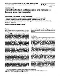
FIG. 1. Site locations for each of the 117 Oklahoma Mesonet sites providing soil data between 1 Mar 2004 and 1 Oct 2005, including Eufaula (square) and Watonga (triangle).

volume is in J m⫺3 or equivalent pressure units. Potential per unit mass is in J kg⫺1 and potential per unit weight is in meters (Marshall et al. 1996, p. 37). Scientists have recognized for some time that the rate of heat dissipation in soil directly relates to the matric potential (e.g., Shaw and Baver 1939). The Campbell Scientific Inc. (CSI) 229-L heat dissipation matric potential sensor installed at Oklahoma Mesonet sites takes advantage of this principle. Encased within a porous ceramic matrix resides a hypodermic needle that houses a resistor as a heating element and a thermocouple as a temperature sensor. The instrument measures an initial soil temperature with the thermocouple, applies a small voltage to the resistance heater for several seconds, and again measures the resulting soil temperature. The difference ⌬T between the initial and final temperatures depends upon the amount of water in the surrounding soil. The instrumentation configuration employed by the Oklahoma Climatological Survey (OCS) yields an absolute temperature measurement error of approximately ⫾1°C. However, since further soil moisture calculations rely instead on a temperature difference, the measured ⌬T likely contains much less error. To remove variability between sensors across the Mesonet, ⌬T relates to a normalized reference temperature for all sensors ⌬Tref according to ⌬Tref ⫽ m⌬T ⫹ b,

共1兲

where m and b are sensor-specific calibration coefficients (Basara and Crawford 2000). Data from vacuum, pressure chamber, and tensiometer measurements of soils (Reece 1996) yield an empirical relationship between the normalized reference temperature and matric potential given by

␺ ⫽ ⫺c exp共a⌬Tref兲,

共2兲

where ␺ is the matric potential (kPa) and a and c are calibration constants equal to 1.788°C⫺1 and 0.717 kPa, respectively. Compared with both the original formulation that appears in Reece (1996) and a modified version from Basara and Crawford (2000), this relationship is simpler and more accurate (B. G. Illston 2005, personal communication). While matric potential provides an important measure of soil moisture for modeling water movement within the soil and from the soil to plants, volumetric water content provides forecast models with important information regarding the volume of water present within the soil as a fraction of the total soil volume. Land surface models rely on measures of volumetric water content to determine soil thermal conductivity and model hydrology. A soil water retention curve describes the relationship between volumetric water content and matric potential for a given soil type (e.g., Clapp and Hornberger 1978; Rawls et al. 1982). Because of the large number of sensors at different depths and different observing sites, OCS decided not to determine a soil water retention curve for each sensor at each site. Instead, an empirical relationship based on detailed soil characteristics and bulk density measurements at each observing site provides coefficients ␣ (kPa⫺1) and n characteristic to each soil texture (Arya and Paris 1981). This same methodology also provides estimates of the residual water content, ⌰r, and the saturated water content, ⌰s, both measured in units of m3water m⫺3 soil. The residual water content represents the volumetric water content of very dry soil and the saturated water content, or porosity, represents the maximum amount of water that a given soil volume can hold. These quantities provide estimates of the soil volumetric water content from calculated values of matric potential using

372


⌰ ⫽ ⌰r ⫹

⌰s ⫺ ⌰r

兵1 ⫹ 关␣共⫺␺Ⲑ100兲兴其

n 1⫺1Ⲑn

,

共3兲

where ⌰ is the volumetric water content and ⌰r is specifically defined as the water content for which the gradient ⳵⌰/⳵␺ becomes zero (van Genuchten 1980).

b. Soil temperature measurements All Mesonet sites employ a Fenwal thermistor to measure soil temperature at 30-s intervals at a depth of 10 cm under both bare soil and native vegetation. Recorded soil temperature observations represent an average of these measurements over 15 min. Approximately half of the Mesonet sites measure soil temperature at a depth of 5 cm under both bare soil and native vegetation and at a depth of 30 cm under native vegetation. Brock et al. (1995) note that the shadow of the solar panel from the Mesonet tower occasionally affects soil temperature readings at the 5-cm depth. In addition, vegetation cover may moderate the response of soil temperature sensors (Fiebrich and Crawford 2001). Allowing for the inherent difficulty with consistently maintaining a completely vegetation-free area over thermistors buried under bare soil, and because the Eta Model accounts for vegetation cover, all soil temperatures in this study represent those measured under native vegetation.

4. Comparison with observations Point measurements of soil temperature and moisture are not as spatially representative as atmospheric measurements, primarily due to spatial heterogeneities in vegetation coverage and soil types (Marshall et al. 2003; Brotzge and Crawford 2003). For this reason, some authors choose to average observations spatially and temporally to reduce small-scale noise and enable model validation and intercomparisons (e.g., Marshall et al. 2003; Robock et al. 2003). One method involves interpolating observations to a model grid, which unfortunately yields comparisons that are partly a function of the interpolation scheme rather than the underlying observations. An analysis scheme cannot account for small spatial variations in the observations and thus analyzed and observed values may differ considerably (Schlatter 1975). Moreover, individual observation points, and not areal averages, provide the raw data for objective analysis schemes that produce gridded initial conditions for models. It is therefore important to correctly estimate point values of soil temperature and soil moisture in the Eta Model so that these values can provide meaningful initial conditions for other numerical models with different grid sizes.

VOLUME 9

Gridded 40-km Eta Model analyses of soil temperature and moisture at 0000 and 1200 UTC are bilinearly interpolated to Oklahoma Mesonet sites in a verification approach that permits a comparison between model grid values and point measurements. While Eta Model soil analyses are available at the present operational grid spacing of 12 km, researchers seldom use these analyses for initializing forecast models. Comparisons span the period from 1 March 2004 through 1 October 2005. This period is sufficient to characterize the performance of the EDAS soil temperature and moisture schemes both before and after the change from continuously self-cycling modeled precipitation to assimilation of precipitation observations on 3 May 2005. Accuracy measures derive from the difference between the observed and modeled values of soil temperature or soil moisture at each individual observation site. The root-mean-squared error (RMSE) averages the squared errors between the Eta Model analyses and observations at each site and is a common accuracy measure that represents a typical error magnitude for forecast errors. The bias provides information on the average error between Eta Model analyses and observations across Oklahoma, though it does not provide information on typical error magnitudes and is not in itself an accuracy measure (Wilks 2006, 279–280). The choice to average errors from point comparisons in this study rather than interpolate the observations to the model grid permits a bulk characterization of the model performance over all of Oklahoma without introducing errors via an objective analysis scheme. This approach is similar to other studies that compare model output and observations (e.g., Crawford et al. 2000, 2001; Santanello and Carlson 2001; Robock et al. 2003). Each soil temperature and moisture observation at an Oklahoma Mesonet site represents a single value at a specific location and depth. Several studies report that soil moisture varies widely over very small horizontal and vertical scales, primarily due to variations in soil type, slope, vegetation cover, and rainfall gradients, while many spatial patterns of soil moisture remain stable over time (e.g., Famiglietti et al. 1999; Mohanty and Skaggs 2001; Teuling et al. 2006). Point measurements of soil temperature are likely more representative of the surrounding area compared with soil moisture, though the spatial structure of temperature in the top soil layer tends to match that of the soil moisture field (Vauclin et al. 1982). The Eta Model analysis grids, on the other hand, represent approximately 40km2 horizontal areas and depths of several centimeters and cannot possibly capture the small-scale variability inherent in the actual soil fields. With this in mind, the overall soil temperature and moisture values in Eta

JUNE 2008


373

FIG. 2. Soil temperature (K) at 0000 UTC 15 Jul 2005 from (a) Oklahoma Mesonet observations at a depth of 5 cm under sod and (b) the 0–10-cm soil layer of the 0000 UTC Eta Model analysis.

Model analyses should still appropriately characterize the bulk soil properties over the entire state of Oklahoma, even if point measurements serve as verification for the model. Though comparisons between the Eta Model and observations only consider point measurements, Figs. 2 and 3 provide informative visualizations of the geo-

graphic variability of Oklahoma Mesonet 5-cm soil temperature and moisture observations compared with Eta Model 0–10-cm soil temperature and moisture analyses. These examples show a representative summer day that exhibits errors similar to the average error across Oklahoma for the entire 18-month period of study. The Oklahoma Mesonet observations are inter-

374


VOLUME 9

FIG. 3. Soil moisture (m3 m⫺3) at 0000 UTC 15 Jul 2005 from (a) Oklahoma Mesonet observations at a depth of 5 cm and (b) the 0–10-cm soil layer of the 0000 UTC Eta Model analysis.

polated to a 3-km horizontal grid using a two-pass Barnes analysis (Barnes 1973). The Eta Model analyses, shown here interpolated to the same 3-km horizontal grid, display a warm and dry bias typical of many 0000 UTC analyses. In addition, the differences in the patterns of each field can influence the subsequent forecast.

The Noah LSM within the EDAS contains four soil layers representing depths of 0–10, 10–40, 40–100, and 100–200 cm, along with a constant reservoir temperature at 300 cm. The physical equations in the Noah LSM predict the soil temperature and soil moisture at the midpoint of each soil layer. Soil temperatures in the 0–10-cm model layer are compared with Oklahoma

JUNE 2008


FIG. 4. Point calculations of daily soil temperature bias (°C) averaged over all of Oklahoma in the 0–10-cm layer from 0000 (gray) and 1200 UTC (black) Eta Model analyses compared with 5-cm soil temperature observations from the Oklahoma Mesonet.

FIG. 5. Daily statewide average 5-cm soil temperature observations from the Oklahoma Mesonet (solid line) and ⫾1 std dev (shaded area) at (a) 0000 and (b) 1200 UTC.

375

376


FIG. 6. Point calculations of daily soil temperature bias (°C) averaged over all of Oklahoma in the 10–40-cm layer from 0000 (gray) and 1200 UTC (black) Eta Model analyses compared with 30-cm soil temperature observations from the Oklahoma Mesonet.

FIG. 7. Daily statewide average 30-cm soil temperature observations from the Oklahoma Mesonet (solid line) and ⫾1 std dev (shaded area) at (a) 0000 and (b) 1200 UTC.

VOLUME 9

JUNE 2008


377

Mesonet observations at a depth of 5 cm, and soil temperatures in the 10–40-cm model layer are compared with observations at a depth of 30 cm. This 30-cm soil temperature observation is as close as possible to the midpoint of the second model soil layer using existing Oklahoma Mesonet instrumentation. For soil moisture, the values from the Eta Model analysis in the 0–10-, 10–40-, and 40–100-cm layers are compared with observations at depths of 5, 25, and 60 cm, respectively. Though the 75-cm soil moisture measurement is closer to the midpoint of the third model soil layer, these observations suffer from errors caused by installation problems (Basara and Crawford 2000) and pass quality assurance tests much less frequently than measurements at the 60-cm depth. Moreover, the annual cycle of statewide averaged soil moisture reveals that soil moisture at both of these levels behaves similarly (Illston et al. 2004). The comparisons between observations and each model layer allow computation of RMSE and bias across the entire Oklahoma Mesonet.

a. Soil temperature There is a strong positive soil temperature bias (forecasts minus observations) in the 0–10-cm layer from 0000 UTC Eta Model analyses compared with observations of 5-cm soil temperatures from all Oklahoma Mesonet sites (Fig. 4). Twelve hours later at 1200 UTC, there is a predominately negative bias. The conspicuous spike representing the 1200 UTC 6 March 2005 bias is a notable exception that depicts an analysis problem for the Oklahoma-wide soil temperatures in the 0–10-cm layer. Overall, the bias for this most shallow soil layer is 4.1°C (⫺1.0°C) and the RMSE is 5.0°C (2.4°C) for 0000 UTC (1200 UTC) Eta Model analyses. Associated skin temperature errors of this magnitude can produce errors in upward longwave radiation of over 20 W m⫺2 during the summer. Modeled soil temperatures at both 0000 and 1200 UTC differ substantially from the observed soil temperatures across Oklahoma, and the statewide average modeled soil temperature frequently exceeds the envelope given by the observed statewide average plus or minus one standard deviation (Fig. 5). Indeed, the overall soil temperature bias for this layer at 0000 UTC exceeds the largest daily standard deviation of 3.66°C for statewide 0000 UTC soil temperature observations during the entire period of study. Summertime 5-cm soil temperature observations generally exhibit more variability across Oklahoma than those in the winter, presumably due to the influence of vegetation and convective rainfall on soil temperatures at this depth. Errors appear reduced in magnitude in the deeper 10–40-cm soil layer, and the 0000 and 1200 UTC soil temperature analyses differ only slightly (Fig. 6).

FIG. 8. Comparative measures between a control model simulation and a model simulation with randomly perturbed soil temperatures showing (a) root-mean-square difference and (b) anomaly correlation for the 0–10-cm layer (black) and the 10–40cm layer (gray).

There is a temporally coherent pattern of errors throughout the year such that errors of the same sign persist for multiweek periods. This trend appears to follow the more variable pattern of daily biases in the upper soil layer. The modifications to the land surface model on 3 May 2005 do not appear to affect significantly the magnitude of subsequent soil temperature errors. The variability of the statewide soil temperatures in this layer is less than that of the upper soil layer. While less than those in the 0–10-cm layer, these errors still represent a substantial fraction of the total variability in the observed statewide soil temperatures in the 10–40-cm model layer (Fig. 7). While the physical equations predict the soil temperature at the midpoint of a given soil layer, soil temperatures in the Eta Model physically represent an average in that layer. A more strict comparison with observations therefore requires an integrated soil temperature throughout a layer rather than point measurements at a specific depth. A cubic spline interpolation between observations of skin temperature and soil tem-

378


VOLUME 9

FIG. 9. Point calculations of daily soil moisture bias (m3 m⫺3) averaged over all of Oklahoma in the 0–10-cm layer from 0000 (gray) and 1200 UTC (black) Eta Model analyses compared with 5-cm soil moisture observations from the Oklahoma Mesonet.

perature at depths of 5 and 10 cm, summed over 5-mm increments, allows an estimate of the soil temperature in the 0–10-cm layer. This integrated soil temperature compares well with the 5-cm soil temperature observa-

tions. The average difference between the integrated and observed temperatures is only 0.23°C with a standard deviation of 0.66°C. The daily difference between the Oklahoma-wide 0–10-cm soil temperature bias in


JUNE 2008

379



Eta Model analyses calculated from either direct measurements at 5 cm or an integrated temperature in the layer may reach as high as 2°C. However, the overall error statistics for the 0–10-cm layer calculated using an integrated soil temperature do not change substantially compared with the direct measurements shown in Fig. 4. Results from a three-dimensional simulation using the fifth-generation Pennsylvania State University– National Center for Atmospheric Research (PSU– NCAR) Mesoscale Model (MM5, version 3.6; Dudhia 1993; Grell et al. 1995; Dudhia 2003) illustrate the importance of initial soil temperature conditions. A test compares a 48-h control forecast on a 3-km horizontal grid over Oklahoma initialized with a 1200 UTC Eta Model analysis on 3 May 2004 with a second forecast with the same initial conditions except that the soil temperature at each grid point in the 0–10-cm layer is perturbed by a uniform random number (Bratley et al. 1987, chapter 6) bounded by ⫾2°C. For consistency with the lower soil layers, the soil temperature in the 10–40-cm layer is perturbed by half the magnitude of the perturbation in the top soil layer. The root-meansquared difference between the perturbed forecast compared with the control forecast shows that the magnitude of the difference between the perturbed soil temperatures and those in the control forecast decreases over the length of the forecast period (Fig. 8a). Because of external influences on the top soil layer,

perturbed soil temperatures in the 0–10-cm layer return to control forecast soil temperatures more quickly over time than temperatures in the 10–40-cm layer. An anomaly correlation, given by m

兺关共T

p

AC ⫽

冋兺

⫺ Tc兲|t⫽0共Tp ⫺ Tc兲|t⫽h兴

n⫽1

m

n⫽1

m

共Tp ⫺ Tc兲 |t⫽0 2

兺共T

n⫽1

p

册

1Ⲑ2

⫺ Tc兲 |t⫽h 2

,

共4兲 where Tp is the perturbed soil temperature and Tc is the control soil temperature at grid point n, summed over m grid points for each forecast hour t over h forecast hours, provides a measure of association between the control and perturbed forecast fields (Wilks 2006, p. 311). Here, the sign and magnitude of the perturbation at forecast time h are compared against the value of the initial perturbation at each grid point. The anomaly correlation at each forecast hour for both soil levels reveals that the sign of each perturbation strongly persists throughout the forecast period (Fig. 8b). Perturbations persist because horizontal diffusion between adjacent gridded soil temperature values is negligible compared with horizontal diffusion in the atmosphere. This test indicates that inaccurate soil temperatures, such as the biased soil temperatures in Eta Model analyses, provided as initial conditions from gridded

380


VOLUME 9

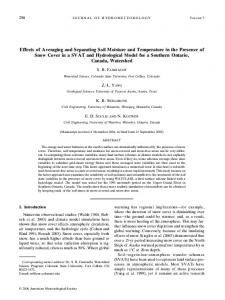
FIG. 12. USDA soil texture triangle displaying measured particle-size fractions for each Oklahoma Mesonet site at multiple depths (dots) for modeled (a) sand (S), (b) silty loam (SL), (c) sandy loam (SL), (d) loam (L), (e) silty clay loam (SiCL), (f) clay loam (CL), and (g) clay (C). The radius of the circle (black) centered on each modeled soil texture class is equal to the mean three-dimensional Euclidean distance between the observed and modeled soil characteristics, with the shaded area representing ⫾1 std dev about the mean. The number of correctly modeled points and the total number of points assigned to each soil texture are separated by a solidus above and to the left of each triangle.

analysis fields may adversely affect the resulting shortterm model forecasts of near-surface variables.

b. Soil moisture There is a pervasive and persistent dry bias in both the 0000 and 1200 UTC Eta Model soil moisture analyses. For each day, the Oklahoma-wide average soil moisture in the 0–10-cm model layer of the Eta Model analyses is generally drier than the observations at 5 cm (Fig. 9). In the 10–40-cm layer, the soil moisture bias slightly exceeds zero for only a single 0000 UTC Eta Model analysis and in the 40–100-cm layer, the soil moisture bias never becomes positive over the period of study (Figs. 10 and 11). Overall, the bias for each soil layer is ⫺0.03, ⫺0.05, and ⫺0.09 m3 m⫺3 and the RMSE

is 0.06, 0.08, and 0.11 m3 m⫺3 for the 0–10-, 10–40-, and 40–100-cm Eta Model layers, respectively. In the 40– 100-cm Eta Model layer, the daily average soil moisture error across all of Oklahoma reaches as large as 35% of the typical range of soil moisture when compared with observations at a depth of 60 cm. There is notable improvement in the analyzed soil moisture fields after the change from self-cycling precipitation to observed precipitation assimilation on 3 May 2005. While this change reduced the magnitude of the errors, and evidences itself as a large discontinuity in the bias time series of Figs. 10 and 11, a strong dry bias persists in the soil moisture field. A portion of this bias may result from the specification of soil texture in the Noah LSM. Soil texture pro-

JUNE 2008


381

FIG. 12. (Continued)

vides critical information on the field capacity and wilting point of the soil, and therefore restricts the range of volumetric water content that a particular soil type can achieve. A careful examination of soil moisture errors in Eta Model analyses requires a comparison between modeled and observed soil textures at Oklahoma Mesonet sites. For such a comparison, the following method assigns particle-size fractions to the midpoint of each Noah LSM soil texture class following Miller and White (1998). Where measurements exist, the observed sand, silt, and clay fractions at four different depths at each Oklahoma Mesonet site are plotted on the standard U.S. Department of Agriculture (USDA) soil texture triangle for each modeled soil texture at the closest model grid point to the Mesonet sites (Fig. 12). The three-dimensional Euclidean distance between the observed and modeled sand, silt, and clay fractions provides a measure of accuracy between the modeled and observed soil textures. The average distance and plus or minus one standard deviation about this average is

shown by the circles centered on the midpoint of the modeled soil texture in each USDA soil texture triangle. For all seven modeled soil texture classes, the Noah LSM correctly classifies less than one-third of the observed soil textures, with the average distance on the soil texture triangle often falling outside the intended classification, though the observed particle-size fractions provide a rather small sample size for most modeled texture classes.

5. Discussion Systematic biases clearly exist in both soil temperature and soil moisture. Consistent with the results of Marshall et al. (2003), soil temperatures in the most shallow soil layer tend to be too warm at 0000 UTC and too cool at 1200 UTC. Positive soil temperature errors in 0000 UTC Eta Model analyses likely stem in part from the documented excess of solar radiation during the daytime (Zamora et al. 2005), while the generally

382


VOLUME 9

FIG. 13. Observed soil moisture at 1200 UTC at Eufaula (gray) at depths of (a) 5, (b) 25, and (c) 60 cm compared with 1200 UTC Eta Model analyses (black) in the 0–10-, 10–40-, and 40–100-cm soil layers, respectively, and observed daily (0000–0000 UTC) precipitation totals (bars).

negative soil temperature biases in 1200 UTC Eta Model analyses result from underestimated downward longwave radiative fluxes during nighttime hours (Stensrud et al. 2006). The modifications to the land surface physics on 3 May 2005 did not mitigate these errors; soil temperatures in the top soil layer remain too high in the 0000 UTC Eta Model analyses and dry soil moisture biases continue in each of the top three soil layers. Tests indicate that these systematic biases in both soil temperature and moisture do not appear to be strongly dependent upon particular soil texture or vegetation types defined in Eta Model grid cells.

At the Eufaula Oklahoma Mesonet site, the EDAS soil moisture errors in the top two model layers result from both an inappropriate response to rainfall events and accelerated desiccation of the soil compared with observations, particularly in the 10–40-cm layer (Fig. 13). The response to precipitation in the 40–100-cm layer appears limited except after several consecutive days of heavy precipitation. The new precipitation assimilation procedure implemented on 3 May 2005 somewhat improved soil moisture estimates at some Mesonet sites, though systematic dry biases remain in the Eta Model analyses.

JUNE 2008


Soil texture classification problems no doubt contribute to the soil moisture errors in Eta Model analyses, but if soil textures were the sole cause of soil moisture errors in Eta Model analyses, one would expect both positive and negative biases. Since the model is overwhelmingly dry in its depiction of soil moisture, these errors are likely the fault of some other mechanism. Regardless of the accuracy of the modeled soil textures, if the modeled volumetric water content is incorrect, then the model cannot possibly provide accurate nearsurface forecasts. Moreover, soil characteristics vary on a scale of a few meters or less, such that particle-size fractions determined from soil cores several meters away from those used for this comparison could yield very different soil texture classifications. Until operational model grid resolutions shrink to the scale of meters, and soil texture data also become available at this resolution, model forecasts will continue to rely upon imperfect soil texture information. Since soil temperature depends strongly on soil moisture, an exploration of the influence of soil heat capacity can help to address the effect of an apparent dry bias on modeled soil temperatures. Soil heat capacity is a function of soil moisture and directly affects the diagnosis of soil temperature. Underestimates of soil moisture such as those in Eta Model analyses could therefore result in poorly estimated soil temperatures. A simple, one-layer slab soil model driven by Oklahoma Mesonet observations allows approximate calculations of the influence of errors in soil moisture alone on soil temperature. Following the formulation in the Noah LSM (Chen and Dudhia 2001), the composite soil volumetric heat capacity employed in the slab model is Cg ⫽ ␪Cwater ⫹ 共1 ⫺ ␪s兲Csoil ⫹ 共␪s ⫺ ␪兲Cair,

共5兲

where ␪ is the soil volumetric water content, Cwater ⫽ 4.2 ⫻ 106 J m⫺3 K⫺1, Csoil ⫽ 1.26 ⫻ 106 J m⫺3 K⫺1, and Cair ⫽ 1004 J m⫺3 K⫺1 are the volumetric heat capacities of water, soil, and air, respectively, and ␪s is the soil porosity. The soil porosity depends upon the soil texture (Cosby et al. 1984) determined from soil cores at each observation site. The slab model predicts the soil temperature T at a depth of 5 cm using a traditional diffusion equation for soil temperature, Cgds

⭸T ⫽ QGS, ⭸t

共6兲

where QGS is the storage ground heat flux and ds ⫽ 10 cm is the depth of the slab. Since the observation frequency for soil temperature is 15 min and that for soil moisture is 30 min, the slab model linearly interpolates the soil moisture observations to obtain a complete time series of data at 15-min intervals. Unfortunately,

383

FIG. 14. Slab soil model temperatures (°C) initialized by (a) 0000 and (b) 1200 UTC 5-cm soil temperature observations at Watonga on 20 Jul 2004. Soil moisture errors of ⫹0.1 (dotted) and ⫺0.1 m3 m⫺3 (dashed) yield temperatures that differ from observed soil temperatures (solid).

the Oklahoma Mesonet sensors do not directly measure the storage ground heat flux, and instead obtain the best possible estimate based on soil temperature, soil moisture, and average soil properties at selected Mesonet sites. When using Eq. (6) with estimated QGS, the observed volumetric water content value, and an initial soil temperature equal to the observed value at 5 cm, the slab model produces soil temperatures that slowly diverge from observations. For this reason, an improved estimate of QGS is calculated by determining the value of QGS needed to produce the observed 5-cm soil temperature, given the observed volumetric water content. The sensitivity of the slab model to errors in the volumetric water content is explored using the improved estimates of QGS for each 15-min period. Ground temperatures from model simulations produced for equal positive and negative volumetric water content biases are compared with observations. While this simple model does not account for the influence of differing soil moisture on the storage ground heat flux or the

384


surface energy balance, it represents an idealized approach to determine the effect of soil moisture errors on soil temperature forecasts. Given observations and soil characteristics at the Watonga Oklahoma Mesonet site for 72 h beginning at both 0000 and 1200 UTC 20 July 2004, this simple onelayer slab soil model estimates the 5-cm soil temperatures that would develop if the observed 5-cm soil moisture error were equal to ⫾0.1 m3 m⫺3 (Fig. 14), or twice the soil moisture error seen in the Eta Model analyses. Different initialization times show the effect of a soil moisture bias on each part of the diurnal cycle. Results reveal that negative soil moisture biases alone may account for more than 1.6°C increases (decreases) in maximum (minimum) daily soil temperatures. Positive soil moisture biases account for a more modest reduction of about 0.9°C in the amplitude of the diurnal soil temperature cycle. While underestimates of soil moisture may contribute to the sign of the soil temperature errors shown in Fig. 4, soil moisture alone apparently cannot account for the magnitude of the soil temperature errors in Eta Model analyses.

6. Conclusions This investigation compares soil temperature and soil moisture estimates from 40-km Eta Model analyses at several different model levels with observations from the Oklahoma Mesonet. In contrast to the findings of Robock et al. (2003), strong biases in soil temperature exist, as well as a severe underestimation of soil moisture at all depths. Soil temperatures in the top soil layer are often too warm at 0000 UTC and too cool at 1200 UTC. As previous studies have shown, soil temperature and soil moisture estimates strongly impact forecasts by numerical weather prediction models that implement sophisticated land surface parameterizations. Problems with soil fields in Eta Model analyses, which provide initial conditions for a variety of research and operational modeling applications, may negatively impact the resulting model forecasts. These existing biases suggest the strong need for an extensive network of soil observations, in addition to atmospheric surface observations, and the necessity for assimilating those observations into land surface initializations. Further research into the reasons for the inappropriate response of the Noah LSM to rainfall events may lead to significant improvements in model performance. Acknowledgments. The authors wish to thank the Oklahoma Climatological Survey for providing Oklahoma Mesonet data and Drs. Peter Lamb and Lance Leslie and three anonymous reviewers for their helpful

VOLUME 9

comments. Funding was provided under NSF Grant ATM-0243720 and by NOAA/Office of Oceanic and Atmospheric Research under NOAA–University of Oklahoma Cooperative Agreement No. NA17RJ1227, U.S. Department of Commerce. REFERENCES Arya, L. M., and J. F. Paris, 1981: A physioempirical model to predict the soil moisture characteristic from particle-size distribution and bulk density data. Soil Sci. Soc. Amer. J., 45, 1023–1030. Barnes, S. L., 1973: Mesoscale objective analysis using weighted time-series observations. NOAA Tech. Memo. ERL NSSL62, National Severe Storms Laboratory, Norman, OK, 60 pp. [NTIS COM-73-10781.] Basara, J. B., and T. M. Crawford, 2000: Improved installation procedures for deep-layer soil moisture measurements. J. Atmos. Oceanic Technol., 17, 879–884. Beljaars, A. C. M., P. Viterbo, M. J. Miller, and A. Betts, 1996: The anomalous rainfall over the United States during July 1993: Sensitivity to land surface parameterization and soil moisture anomalies. Mon. Wea. Rev., 124, 362–383. Betts, A. K., J. H. Ball, A. C. M. Beljaars, M. J. Miller, and P. A. Viterbo, 1996: The land-surface-atmosphere interaction: A review based on observational and global modeling perspectives. J. Geophys. Res., 101, 7209–7226. Bhumralkar, C. M., 1975: Numerical experiments on the computation of ground surface temperature in an atmospheric general circulation model. J. Appl. Meteor., 14, 1246–1258. Black, T. L., 1994: The new NMC mesoscale Eta Model: Description and forecast examples. Wea. Forecasting, 9, 265–278. Blackadar, A. K., 1976: Modeling the nocturnal boundary layer. Preprints, Third Symp. on Atmospheric Turbulence, Diffusion, and Air Quality, Raleigh, NC, Amer. Meteor. Soc., 46– 49. Bratley, P., B. L. Fox, and L. E. Schrage, 1987: A Guide to Simulation. 2nd ed. Springer-Verlag, 397 pp. Brennan, M. J., G. M. Lackmann, and S. E. Koch, 2003: An analysis of the impact of a split-front rainband on Appalachian cold-air damming. Wea. Forecasting, 18, 712–731. Bright, D. R., and S. L. Mullen, 2002: The sensitivity of the numerical simulation of the southwest monsoon boundary layer to the choice of PBL turbulence parameterization in MM5. Wea. Forecasting, 17, 99–114. Brock, F. V., K. C. Crawford, R. L. Elliot, G. W. Cuperus, S. J. Stadler, H. L. Johnson, and M. D. Eilts, 1995: The Oklahoma Mesonet: A technical overview. J. Atmos. Oceanic Technol., 12, 5–19. Brotzge, J. A., and K. C. Crawford, 2003: Examination of the surface energy budget: A comparison of eddy correlation and Bowen ratio measurement systems. J. Hydrometeor., 4, 160– 178. Chen, F., and J. Dudhia, 2001: Coupling an advanced land surface–hydrology model with the Penn State–NCAR MM5 modeling system. Part I: Model implementation and sensitivity. Mon. Wea. Rev., 129, 569–585. ——, and Coauthors, 1996: Modeling of land-surface evaporation by four schemes and comparison with FIFE observations. J. Geophys. Res., 101, 7251–7268. Chen, Y., F. L. Ludwig, and R. L. Street, 2004: Stably stratified

JUNE 2008


flows near a notched transverse ridge across the Salt Lake valley. J. Appl. Meteor., 43, 1308–1328. Clapp, R. B., and G. M. Hornberger, 1978: Empirical equations for some soil hydraulic properties. Water Resour. Res., 14, 601–604. Clark, C. A., and R. W. Arritt, 1995: Numerical simulations of the effect of soil moisture and vegetation cover on the development of deep convection. J. Appl. Meteor., 34, 2029–2045. Colle, B. A., C. F. Mass, and D. Ovens, 2001: Evaluation of the timing and strength of MM5 and Eta surface trough passages over the eastern Pacific. Wea. Forecasting, 16, 553–572. Cosby, B. J., G. M. Hornberger, R. B. Clapp, and T. R. Ginn, 1984: A statistical exploration of the relationships of soil moisture characteristics to the physical properties of soils. Water Resour. Res., 20, 682–690. Crawford, T. M., D. J. Stensrud, T. N. Carlson, and W. J. Capehart, 2000: Using a soil hydrology model to obtain regionally averaged soil moisture values. J. Hydrometeor., 1, 353–363. ——, ——, F. Mora, J. W. Merchant, and P. J. Wetzel, 2001: Value of incorporating satellite-derived land cover data in MM5/ PLACE for simulating surface temperatures. J. Hydrometeor., 2, 453–468. Deardorff, J. W., 1978: Efficient prediction of ground surface temperature and moisture, with inclusion of a layer of vegetation. J. Geophys. Res., 83, 1889–1903. DiMego, G. J., and E. Rogers, cited 2005: Spring 2005 upgrade package for North American Mesoscale (NAM) decision brief. [Available online at http://wwwt.emc.ncep.noaa.gov/ mmb/Spring2005.NAMUpgrade.pdf.] Dirmeyer, P. A., F. J. Zeng, A. Ducharne, J. C. Morrill, and R. D. Koster, 2000: The sensitivity of surface fluxes to soil water content in three land surface schemes. J. Hydrometeor., 1, 121–134. Dudhia, J., 1993: A nonhydrostatic version of the Penn State– NCAR mesoscale model: Validation tests and simulation of an Atlantic cyclone and cold front. Mon. Wea. Rev., 121, 1493–1513. ——, 1996: A multi-layer soil temperature model for MM5. Preprints, Sixth PSU/NCAR Mesonet Model Users’ Workshop, Boulder, CO, NCAR, 49–50. ——, 2003: MM5 model status and plans. Preprints, 13th PSU/ NCAR Mesoscale Model Users’ Workshop, Boulder, CO, NCAR, 1–2. Ek, M. B., and A. A. M. Holtslag, 2004: Influence of soil moisture on boundary layer cloud development. J. Hydrometeor., 5, 86–99. Entekhabi, D., and Coauthors, 1999: An agenda for land surface hydrology research and a call for the second international hydrological decade. Bull. Amer. Meteor. Soc., 80, 2043–2058. Entin, J. K., A. Robock, K. Y. Vinnikov, S. E. Hollinger, S. Liu, and A. Namkhai, 2000: Temporal and spatial scales of observed soil moisture variations in the extratropics. J. Geophys. Res., 105, 11 865–11 877. Famiglietti, J. S., and Coauthors, 1999: Ground-based investigation of soil moisture variability within remote sensing footprints during the Southern Great Plains 1997 (SGP97) Hydrology Experiment. Water Resour. Res., 35, 1839–1851. Fennessy, M. J., and J. Shukla, 1999: Impact of initial soil wetness on seasonal atmospheric prediction. J. Climate, 12, 3167– 3180. Fiebrich, C. A., and K. C. Crawford, 2001: The impact of unique meteorological phenomena detected by the Oklahoma Me-

385

sonet and ARS Micronet on automated quality control. Bull. Amer. Meteor. Soc., 82, 2173–2187. ——, J. E. Martinez, J. A. Brotzge, and J. B. Basara, 2003: The Oklahoma Mesonet’s skin temperature network. J. Atmos. Oceanic Technol., 20, 1496–1504. Fulton, R. A., J. P. Breidenbach, D.-J. Seo, D. A. Miller, and T. O’Bannon, 1998: The WSR-88D rainfall algorithm. Wea. Forecasting, 13, 377–395. Galewsky, J., and A. Sobel, 2005: Moist dynamics and orographic precipitation in northern and central California during the New Year’s flood of 1997. Mon. Wea. Rev., 133, 1594–1612. Gannon, P. T., 1978: Influences of earth surface and cloud properties in the south Florida sea breeze. NOAA Tech. Rep. ERL402-NHELM2, 91 pp. [NTIS PB-297398.] Gao, X., S. Sorooshian, and H. V. Gupta, 1996: A sensitivity analysis of the Biosphere-Atmosphere Transfer Scheme (BATS). J. Geophys. Res., 101, 7279–7289. Grell, G. A., J. Dudhia, and D. R. Stauffer, 1995: A description of the fifth-generation Penn State/NCAR Mesoscale Model (MM5). Tech. Note NCAR/TN-398⫹STR, 122 pp. [Available from MMM Division, NCAR, P.O. Box 3000, Boulder, CO 80307.] Hart, K. A., W. J. Steenburgh, D. J. Onton, and A. J. Siffert, 2004: An evaluation of mesoscale-model-based model output statistics (MOS) during the 2002 Olympic and Paralympic Winter Games. Wea. Forecasting, 19, 200–218. Hoadley, J. L., K. Westrick, S. A. Ferguson, S. L. Goodrick, L. Bradshaw, and P. Werth, 2004: The effect of model resolution in predicting meteorological parameters used in fire danger rating. J. Appl. Meteor., 43, 1333–1347. Illston, B. G., J. B. Basara, and K. C. Crawford, 2004: Seasonal to interannual variations of soil moisture measured in Oklahoma. Int. J. Climatol., 24, 1883–1896. Koren, V., J. Schaake, K. Mitchell, Q.-Y. Duan, F. Chen, and J. M. Baker, 1999: A parameterization of snowpack and frozen ground intended for NCEP weather and climate models. J. Geophys. Res., 104, 19 569–19 585. Koster, R. D., and Coauthors, 2004: Realistic initialization of land surface states: Impacts on subseasonal forecast skill. J. Hydrometeor., 5, 1049–1063. Leese, J., T. Jackson, A. Pitman, and P. Dirmeyer, 2001: GEWEX/BAHC International Workshop on Soil Moisture Monitoring, Analysis, and Prediction for Hydrometeorological and Hydroclimatological Applications. Bull. Amer. Meteor. Soc., 82, 1423–1430. Lin, Y., K. E. Mitchell, E. Rogers, and G. J. DiMego, 2005: Using hourly and daily precipitation analyses to improve model water budget. Preprints, Ninth Symp. on Integrated Observing and Assimilation Systems for the Atmosphere, Oceans, and Land Surface, San Diego, CA, Amer. Meteor. Soc., 3.3. [Available online at http://ams.confex.com/ams/pdfpapers/ 84484.pdf.] Liu, Y., and R. Avissar, 1999a: A study of persistence in the land–atmosphere system using a general circulation model and observations. J. Climate, 12, 2139–2153. ——, and ——, 1999b: A study of persistence in the land–atmosphere system with a fourth-order analytical model. J. Climate, 12, 2154–2168. ——, D. Z. Ye, and J. J. Ji, 1993: Influence of soil moisture and vegetation on climate. Part II: Numerical experiments on persistence of short-term climatic anomalies. Sci. China, 36B, 102–109.

386


Mahrt, L., and H. L. Pan, 1984: A two-layer model of soil hydrology. Bound.-Layer Meteor., 29, 1–20. Marshall, C. H., K. C. Crawford, K. E. Mitchell, and D. J. Stensrud, 2003: The impact of the land surface physics in the operational NCEP Eta Model on simulating the diurnal cycle: Evaluation and testing using Oklahoma Mesonet data. Wea. Forecasting, 18, 748–768. Marshall, T. J., J. W. Holmes, and C. W. Rose, 1996: Soil Physics. 3rd ed. Cambridge University Press, 453 pp. McCumber, M. C., and R. A. Pielke, 1981: Simulation of the effects of surface fluxes of heat and moisture in a mesoscale numerical model. J. Geophys. Res., 86, 9929–9938. Miller, D. A., and R. A. White, 1998: A conterminous United States multilayer soil characteristics dataset for regional climate and hydrology modeling. Earth Interactions, 2. [Available online at http://EarthInteractions.org.] Mohanty, B. P., and T. H. Skaggs, 2001: Spatio-temporal evolution and time-stable characteristics of soil moisture within remote sensing footprints with varying soil, slope, and vegetation. Adv. Water Resour., 24, 1051–1067. Nelson, J. A., 1999: The Eta Data Assimilation System. WR Tech. Attachment 99-14, 6 pp. [Available from National Weather Service Western Region, P.O. Box 11188, Salt Lake City, UT 84147.] Noilhan, J., and S. Planton, 1989: A simple parameterization of land-surface processes for meteorological models. Mon. Wea. Rev., 117, 536–549. Pan, H. L., and L. Mahrt, 1987: Interaction between soil hydrology and boundary-layer development. Bound.-Layer Meteor., 38, 185–202. Pielke, R. A., and X. Zeng, 1989: Influence on severe storm development of irrigated land. Natl. Wea. Dig., 14, 16–17. ——, G. E. Liston, J. L. Eastman, L. Lu, and M. Coughenour, 1999: Seasonal weather prediction as an initial valve problem. J. Geophys. Res., 104, 19 463–19 479. Rawls, W. J., D. L. Brakensiek, and K. E. Saxton, 1982: Estimation of soil water properties. Trans. Amer. Soc. Agric. Eng., 25, 1316–1320. Reece, C. F., 1996: Evaluation of a line heat dissipation sensor for measuring soil matric potential. Soil Sci. Soc. Amer. J., 60, 1022–1028. Rind, D., 1982: The influence of ground moisture conditions in North America on summer climate as modeled in the GISS GCM. Mon. Wea. Rev., 110, 1487–1494. Robock, A., K. Y. Vinnikov, G. Srinivasan, J. K. Entin, S. E. Hollinger, N. A. Speranskaya, S. Liu, and A. Namkhai, 2000: The global soil moisture data bank. Bull. Amer. Meteor. Soc., 81, 1281–1299. ——, and Coauthors, 2003: Evaluation of the North American Land Data Assimilation System over the southern Great Plains during the warm season. J. Geophys. Res., 108, 8846, doi:10.1029/2002JD003245. Rodell, M., P. R. Houser, A. A. Berg, and J. S. Famiglietti, 2005: Evaluation of 10 methods for initializing a land surface model. J. Hydrometeor., 6, 146–155. Rogers, E., T. L. Black, D. G. Deaven, G. J. DiMego, Q. Zhao, M. Baldwin, N. W. Junker, and Y. Lin, 1996: Changes to the operational “early” eta analysis/forecast system at the National Centers for Environmental Prediction. Wea. Forecasting, 11, 391–413. Rowntree, P. R., and J. A. Bolton, 1983: Simulation of the atmospheric response to soil moisture anomalies over Europe. Quart. J. Roy. Meteor. Soc., 109, 501–526.

VOLUME 9

Santanello, J. A., and T. N. Carlson, 2001: Mesoscale simulation of rapid soil drying and its implications for predicting daytime temperature. J. Hydrometeor., 2, 71–88. Schlatter, T. W., 1975: Some experiments with a multivariate statistical objective analysis scheme. Mon. Wea. Rev., 103, 246– 257. Sellers, P. J., Y. Mintz, Y. C. Sud, and A. Dalcher, 1986: A simple biosphere model (SiB) for use within general circulation models. J. Atmos. Sci., 43, 505–531. Seuffert, G., H. Walker, P. Viterbo, M. Drusch, and J.-F. Mahfouf, 2004: The usage of screen-level parameters and microwave brightness temperature for soil moisture analysis. J. Hydrometeor., 5, 516–531. Shafer, M. A., C. A. Fiebrich, D. S. Arndt, S. E. Fredrickson, and T. W. Hughes, 2000: Quality assurance procedures in the Oklahoma Mesonetwork. J. Atmos. Sci., 17, 474–494. Shaw, B., and L. D. Baver, 1939: Heat conductivity as an index of soil moisture. J. Amer. Soc. Agron., 31, 886–891. Smith, C. B., M. N. Lakhtakia, W. J. Capehart, and T. N. Carlson, 1994: Initialization of soil-water content in regional-scale atmospheric prediction models. Bull. Amer. Meteor. Soc., 74, 585–593. Stensrud, D. J., and S. J. Weiss, 2002: Mesoscale model ensemble forecasts of the 3 May 1999 tornado outbreak. Wea. Forecasting, 17, 526–543. ——, and Coauthors, 2006: The New England high-resolution temperature program. Bull. Amer. Meteor. Soc., 87, 491–498. Teuling, A. J., R. Uijlenhoet, F. Hupet, E. E. van Loon, and P. A. Troch, 2006: Estimating spatial mean root-zone soil moisture from point-scale observations. Hydrol. Earth Syst. Sci., 10, 755–767. Troen, I., and L. Mahrt, 1986: A simple model of the boundary layer: Sensitivity to surface evaporation. Bound.-Layer Meteor., 37, 129–148. van Genuchten, M. T., 1980: A closed-form equation for predicting the hydraulic conductivity of unsaturated soils. Soil Sci. Soc. Amer. J., 44, 892–898. Vauclin, M., S. R. Vieira, R. Bernard, and J. L. Hatfield, 1982: Spatial variability of surface temperature along two transects of a bare soil. Water Resour. Res., 18, 1677–1686. Vinnikov, K. Y., and I. B. Yeserkepova, 1991: Soil moisture: Empirical data and model results. J. Climate, 4, 66–79. ——, A. Robock, N. A. Speranskaya, and C. A. Schlosser, 1996: Scales of temporal and spatial variability of midlatitude soil moisture. J. Geophys. Res., 101, 7163–7174. Viterbo, P., and A. C. M. Beljaars, 1995: An improved land surface parameterization scheme in the ECMWF model and its validation. J. Climate, 8, 2716–2748. ——, and A. K. Betts, 1999: Impact of the ECMWF reanalysis soil water on forecasts of the July 1993 Mississippi flood. J. Geophys. Res., 104, 19 361–19 366. Walker, J. M., and P. R. Rowntree, 1977: The effect of soil moisture on circulation and rainfall in a tropical model. Quart. J. Roy. Meteor. Soc., 103, 29–46. Walsh, J. E., W. H. Jasperson, and B. Ross, 1985: Influence of snow cover and soil moisture on monthly air temperature. Mon. Wea. Rev., 113, 756–768. Wei, M.-Y., Ed., 1995: Soil moisture: Report of a workshop held in Tiburon, California, 25–27 January 1994. NASA Conference Publication 3319, 80 pp. Westrick, K. J., P. Storck, and C. F. Mass, 2002: Description and evaluation of a hydrometeorological forecast system for mountainous watersheds. Wea. Forecasting, 17, 250–262.

JUNE 2008


Wilks, D. S., 2006: Statistical Methods in the Atmospheric Sciences. International Geophysics Series, Vol. 91, Academic Press, 627 pp. Xu, Q., and B. Zhou, 2003: Retrieving soil water contents from soil temperature measurements by using linear regression. Adv. Atmos. Sci., 20, 849–858. Yan, H., and R. A. Anthes, 1988: The effect of variations in surface moisture on mesoscale circulations. Mon. Wea. Rev., 116, 192–208. Yeh, T.-C., R. T. Wetherald, and S. Manabe, 1984: The effect of soil moisture on the short-term climate and hydrology change—A numerical experiment. Mon. Wea. Rev., 112, 474– 490. Zamora, R. J., E. G. Dutton, M. Trainer, S. A. McKeen, J. M. Wilczak, and Y.-T. Hou, 2005: The accuracy of solar irradi-

387

ance calculations used in mesoscale numerical weather prediction. Mon. Wea. Rev., 133, 783–792. Zehnder, J. A., 2002: Simple modifications to improve fifthgeneration Pennsylvania State University–National Center for Atmospheric Research Mesoscale Model performance for the Phoenix, Arizona, metropolitan area. J. Appl. Meteor., 41, 971–979. Zhong, S., H.-J. In, X. Bian, J. Charney, W. Heilman, and B. Potter, 2005: Evaluation of real-time high-resolution MM5 predictions over the Great Lakes region. Wea. Forecasting, 20, 63–81. Ziegler, C. L., W. J. Martin, R. A. Pielke, and R. L. Walko, 1995: A modeling study of the dryline. J. Atmos. Sci., 52, 263–285. Zobler, L., 1986: A world soil file for global climate modeling. NASA Tech. Memo. 87802, 32 pp.