Solid Modeling with Boolean Operations in

Solid Modeling with Boolean Operations in Mathematica. Part 1 : Definition of Solid Objects Robert Kragler Abstract. The intention of this paper is to illustrate the underlying mathematical algorithms involved in constructive solid geometry (CSG). In Part 1, apart from basic primitives (e.g. sphere, cuboid, cylinder, cone pyramid, torus, ellipsoid, hyperboloids and paraboloid) more sophisticated solids are created such as polyhedra, superquadrics and 3d objects either defined by (closed) algebraic surfaces or Boolean functions. These 3d objects are subjected to geometric transformations such as scaling, translation and rotation and thus can be deformed, positioned and oriented at any location in 3d space. Finally, in Part 2 applications are given where solids are combined to more complex objects by application of various Boolean operators. Keywords. Constructive solid geometry, solid objects, Boolean functions, geometric transformations.

Initialization (Mathematica V8.0.4) In order to load the Mathematica package SolidM odeling.m it is required that both the current Mathematica notebook and the package are located in the same subdirectory. Clear["Global ` * "] SetDirectory[NotebookDirectory[]]; Get["SolidModeling ` "] Once, SolidM odeling.m is loaded one has access to an application library which provides about 50 procedures etc. . Names["SolidModeling ` ""*"]// Length 50 In order to save the document as a LAT EX file interactive 3d graphics have to be converted into raster graphics by application of the procedure raster raster. raster= Rasterize[#, ImageResolution → 210]& ; VersionDateTime Mathematica V 8.0.4 for Microsoft Windows (64-bit) (October 7, 2011) date= September14, 2016; time= 00 : 09h

2

Robert Kragler

1. Mathematica package SolidModeling The Mathematica package ( SolidModeling.m SolidModeling.m) contains 16 procedures defineBoolean which describe primitive solids, quadrics, superquadrics and polyhedra; moreover, exploiting the built-in procedure PolyhedronData[,"RegionFunction"] provides the Boolean function representation of more than 150 polyhedra. booleanList = Names["SolidModeling`defineBoolean*"] defineBooleanCone, defineBooleanCuboid, defineBooleanCutter, defineBooleanCylinder, defineBooleanEllipsoid, defineBooleanFunction, defineBooleanHyperboloid, defineBooleanParaboloid, defineBooleanPolyhedron, defineBooleanPrimitive, defineBooleanPyramid, defineBooleanSphere, defineBooleanSuperellipsoid, defineBooleanSuperhyperboloid, defineBooleanSuperparaboloid, defineBooleanSuperquadric, defineBooleanSupertoroid, defineBooleanToroid Moreover, there are 7 binary Boolean operators [g1,g2] and one unary operator complement[g1] which act directly on Boolean functions gi characterizing solids. These Boolean operators are investigated in detail in Part 2. booleanOps = {"complement", "difference", "intersection", "nand", "nor", "symmDifference", "union", "xnor"}; Furthermore, the package contains some auxiliary routines mainly used as shortcuts or abbreviations. miscList= {"arrowAxis","booleanSimplify","cyl","coordSystem", "coordTrans","showCoordSys","cutDir","cutter","cutY", "OpacityDir","plotSolid", "print","rotation","sweep", "VersionDateTime","PackageInfo","fS","lEx","mF","mS","tF"};

2. Prolog CAD systems (see [1], [2a] such as solid modeling systems or volume modeler essentially apply Boolean operations. These mathematical methods used for the construction of 3d solids play an important part in CAD systems for simulation of components too. As regards to the mathematical description of 3d objects several possibilities exist :

2.1. Boundary Representation (B-rep) : In this case [2b] a 3d object is defined by its confining surfaces. B-rep models are preferentially applied for visualization of 3d computer graphics and also in CAD programs because they can be processed algorithmically fast. Furthermore, this method lends itself for the description of volume models too; the object is described by its confining surfaces only where it has to be ensured by an algorithm that the hull is closed.

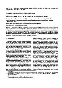
3 3d objects will be defined with the help of a vertex-edge-face graph. The geometry is given by the coordinates of the 3d points; relations between points describe edges and surfaces where, edges reference to point and surfaces to edges. As to the description of 3d-objects three lists are defined : (i) the knot list (containing the coordinates of points) (ii) the edge list (referencing for each edge two points) (iii) the surface list (containing for each surface a closed sequence of edges). Moreover, an unambiguous description requires to define the orientation of each surface patch through its sequence of edges. However, the complete description of a volume model requires an additional table : (iv) the volume list (specifying all surfaces enclosing the body). It must be ensured that the partial surfaces confine the volume completely so that no gaps remain. By means of the orientation it is defined whether the normal vector of the first surface given in the list of boundary surfaces points outwards, i.e. away from the volume, or inwards, i.e. into the volume. With the help of the “right-hand-rule” the surface normal is determined which is used to fix the forefront (exterior side) of a surface; the opposite orientation defines the backfront (interior side) of a surface; it has to be pointed out that the edge order is evaluated. As for surfaces in 2d it is likewise possible in 3d to model objects with holes by inverting the orientation of surface patches. 2.2. Constructive Solid Geometry (CSG) : In this approach [2c] a 3d object is represented by combination of primitive bodies (such as sphere, cuboid, cylinder etc.) by means of Boolean algebra. The button Eval ¯↓ (thanks to David Park) evaluates the closed input cell (option CellOpen →False so that its Mathematica code is hidden) which immediately follows the Eval button. The illustration below shows the action of Boolean operations on a cube and sphere : ( Eval ¯ ↓ )

Fig.1 Basic Boolean operations (union, difference, intersection and negated intersection) union ⇔ A∨B : Union merges objects ( A= cube , B= sphere) into a single object. A, B intersection ⇔ A∧B : Intersection retains only those parts common to both objects (A, B). difference ⇔ A∧(¬B) : Difference cuts parts B from A (here subtract sphere from cube) neg. intersection ⇔ ¬A∧B : Intersection of B (sphere) with ¬A (negated cube) results in the A∧B sphere minus the intersection (A B). This modeling technique of primitive bodies is applied in CAD programs and 3d computer graphics giving rise to the creation of complicated surfaces and solids by application of Boolean operations in order to combine various objects. Hence, objects generated with CSG might look rather complex but are nothing more than 3d objects skillfully combined with each other.

4

Robert Kragler

The basic objects from which CSG bodies are created are called primitive. Typically, these are bodies whose surfaces are described by means of a relatively simple mathematical formula, such as spheres, cones, tori, cuboids, cylinders, prisms and pyramids. In principle, for representing curved surfaces, it is possible for CSG to work with either polygonal meshes or parametric surfaces. The parametric ansatz admits the exact mathematical calculation and representation of bodies whereas polygonal meshes represent only an approximate description of the real object. Generally, a complex body is created with primitives connected through Boolean operations which act on (point-) sets such as union, difference, intersection etc..

3. CSG tree Because concatenated CSG operations generally do not commute they can be hierarchically ordered and transfered into a CSG tree (see [2c])

Fig.2 Hierarchical CSG tree Each leaf corresponds to a primitive body (i.e. a CSG object), and each node represents a new intermediate object produced by a Boolean operation and suitable for further Boolean combinations. ∩ ), unions (∪ ∪ ), and the difference (-). In the figure above, the nodes represent either intersections (∩ The root of the (inverted) tree is the final result.

3.1. Realization of CSG tree with Mathematica The CSG tree above can easily be realized with the help of Mathematica in terms of graphic primitives ( cube, sphere and cylinders) and Boolean operations ( union, intersection and difference). Evaluation of the hidden input cell with Eval ¯↓ shows :

5

Fig.3 Realization of CSG tree with Mathematica Starting from the bottom line there is on the second level the intersection A ∧ B of cube with sphere, and in addition the union A ∨ B of three cylinders oriented along x, y, z direction. The final result A ∧ (¬B) ) of the beveled cube with the cylindrical (i.e. the root) on the third level is the difference differenceA cross. Note : in Euclidean space R3 the Boolean operations ∪, ∩, CE (= complementary set) constitute a so-called Boolean algebra which includes commutativity law. Yet, the difference operator is not part of this Boolean algebra. However, a combination of the operators CE and ∩ are an alternative for the ”\” ”\”- operator, such that A \ B = A ∩ CE B . See also [3]. The resulting solid developed in the example given above can be directly calculated (C ∩ S) ∩ (CE Cx ∩ CE Zy ∩ CE Zz ) (where C =cube, S =sphere, Zx,y,z = cylinder) : Eval ¯↓

Fig.4 Resulting solid : intersection of cube with sphere and 3 cylinders

6

Robert Kragler

4. Geometric transformations Mathematica provides several transformation functions for translation and rotation ————————————————————————————————————————– TranslationTransform[t] gives a transformation representing a translation by a vector t . axis RotationTransform[θ,axis axis] transformation representing 3D rotation with angle θ around the direction axis axis axis. RotationTransform [{P1 , P2 }] rotates vector P1 into direction of vector P2 . ————————————————————————————————————————–

4.1. 3D rotation and translation matrix (for homogeneous coordinates) The usage of homogeneous coordinates {x,y,z,1} has the advantage that translations and rotations can be treated on the same footing. First of all, the translation matrix corresponding to a translation with translational vector t ={ 3, 0,-1 } is given as (T = TranslationTransform[{3, 0, −1}] [[1]])//mF   1 0 0 3  0 1 0 0     0 0 1 −1  0 0 0 1 Second, the rotation transform covering both equivalent descriptions, i.e. the rotation of direction vector P1 into direction P2 or rotation by angle θ around the rotation axis Q is given by ————————————————————————————————————————– rotation[arg1 ,arg2 List] := Module[{}, Clear[RT]; If[VectorQ[arg1] === True, RT = RotationTransform[ RotationTransform[{{arg1,arg2 arg1,arg2}}], (* {P1,P2} *) RT = RotationTransform[arg1,arg2] ]; (* {θ, Q} *) Return[RT] ]; ————————————————————————————————————————– The rotation matrices for : (i) rotation of P1 = { 0, 0, 1 } into direction P2 = { 1, 0, 1 } and (ii) rotation with angle θ = π/4 about axis = { 0, 1, 0 } are the same; the procedure rotation[arg1,arg2] combines both equivalent descriptions. { } {{P1, P2}, θ, axis} = {{0, 0, 1}, {1, 0, 1}}, π4 , {0, 1, 0} ; P1 [[1]] {R1 = RotationTransform RotationTransform[{P1 P1, P2 P2}][[1]] [[1]], [[1]] R2 = RotationTransform RotationTransform[ θ, axis ][[1]] [[1]],

7 P1 [[1]] R = rotation rotation[P1 P1, P2 P2][[1]] [[1]]}; R1 === R2 === R True where the (4 x 4) rotation matrix follows as R// mF 

√1 2

 0   − √1 2 0

0 1 0 0

√1 2

0 √1 2

0

 0 0   0  1

Coordinate substitution {x, y, z, 1} → {ξ, η, ζ, 1} The following is an example of linear transformation of coordinates involving a rotation R and translation T . The resulting transformation matrix M=T.R is the concatenation of a rotation around y-axis by θ = π/4 followed by a translation t = {3, 0, −1} mF /@ {M = T.R, invM = Inverse[(T.R)// mS]}  √   √1 √1  0 √12 3 0 − √12 −2 2  2 2     0 1 0 0  0 0  0 1   √ ,  − √1 0 √1 −1   √1 √1  0 − 2   2 2 2 2   0 0 0 1 0 0 0 1

          

T.R Inverse[T.R T.R] will transform the coordinate system {x, y, z} Thus, using the inverse matrix M−1 = Inverse into the new coordinate system {ξ, η, ζ} //N //Most) (CoordS1 = Evaluate[Thread @ ({x,y,z,1} → invM invM . {ξ, η, ζ, 1})]//N //Most)/. approxRoot//ColumnForm √ x → −2 2 − √ζ2 + √ξ2 y→η√ z → − 2 + √ζ2 + √ξ2 Finally, {ξ, η, ζ} is rewritten by {x, y, z} z}. This coordinate substitution will extensively been used to transform any Boolean function (of primitives which are defined in the coordinate origin) with respect to an arbitrary position in 3d space.

5. Dynamic viewpoint 5.1. viewPointSelector A useful tool for the orientation of a 3d object is viewPointSelector which faciliates the determination of an optimal viewpoint ViewPoint → {sx , sy , sz } ) . Unfortunately, the viewpoint selector implemented in Mathematica V5.2 became obsolete since version 6. However, due to [4] and [5] a procedure is constructed which generates an interactive palette

8

Robert Kragler

————————————————————————————————————————– coords = PolyhedronData["Cube", "VertexCoordinates"]//N ; (* read cube data *) indices = PolyhedronData["Cube", "FaceIndices"]; ncoords = Rescale[coords]; (* Rescale vertex coordinates *) testCube = Graphics3D[{EdgeForm[ ], (* Replace edges by cylinders, vertices by spheres *) GraphicsComplex[7 ∗ ncoords, {({Black, Cylinder[#, .15]}&/@ Partition[Append[#, First[#]], 2, 1])&/@ indices, {Red, Sphere[#, .4]}&/@ Range[Length[ncoords]]} ] }, Boxed → False, ViewAngle → All, ImageSize → 250]; ]) −2) (( [ & n2:= N @ Round # ∗ 1022 10−2 SetOptions[Graphics3D, ViewAngle → 20 Degree]; viewPointSelector[gr Graphics3D]:= DynamicModule[{vp = ViewPoint /.Options[Graphics3D], vv = ViewVertical/.Options[Graphics3D], va = ViewAngle /.Options[Graphics3D]}, Module[{copy}, copy[expr ]:=NotebookPut[Notebook[{ToString[expr]}], ClipboardNotebook[ ] ]; Panel[Column[{Show[gr, ViewPoint → Dynamic[vp], ViewVertical → Dynamic[vv], Ticks → None, Axes → True, LabelStyle → Directive[Bold, FontFamily → "Helvetica", FontSize → 14], AxesStyle → Thread[ List[{Red, Darker[Green], Blue}, AbsoluteThickness[4]]], AxesEdge → {{−1, −1}, {−1, −1}, {−1, −1}}, AxesLabel → {X, Y, Z}, Background → LightBlue, BaseStyle → {FontWeight → Bold, FontFamily → "Helvetica", Italic, 12}, SphericalRegion → True, ImageSize → 250], Grid[{{Button["ViewPoint", copy[vp//n2], BaseStyle → {"GenericButton", 12, Bold}], Dynamic[vp]}, {Button["ViewVertical", copy[vv//n2], BaseStyle → {"GenericButton", 12, Bold}], Dynamic[vv]}

9 }, Alignment → {Left, Baseline}] }], ImageSize → 300] ] ] ————————————————————————————————————————–

5.2. Generation of palette The dynamic 3d graphics above can be casted into a (free movable) palette using : CreatePalette[Style[viewPointSelector[testCube], Deployed → False, Selectable → True], WindowClickSelect → True, Magnification → 1.2, WindowTitle → "viewPointSelector"]; 5.3. Testing viewPointSelector In order to copy the coordinates (changed due to spatial rotation of the wireframe cube) for ViewPoint or ViewVertical one of the buttons must be pushed and then the keyboard sequence CTRL +C to insert the number triple e.g. {-1.46,4.82,0.8} at the cursor position. Eval ¯↓ raster@viewPointSelector[testCube]

Fig.5 Dynamic view point selector

10

Robert Kragler

6. Basic primitives A subset of all basic primitives (see [6] ) with names defineBoolean available in the package SolidModeling.m is listed below : ? defineBoolean* defineBooleanSphere Apart from a sphere (defineBooleanSphere defineBooleanSphere) all other primitives can be subjected to a rotation with respect to the origin either with : (i) (θ, Q ) where θ is the rotation angle and Q is the rotation axist, or equivalently P1 , P2 ) i.e. from axis P1 into direction of P2 . (ii) (P In addition a translation by vector t (default {0,0,0} {0,0,0}) from the origin and scaling by s (default {1,1,1} ) along the the coordinate axes are applicable to every solid. 6.1. Geometric transformation (translation) of a sphere (defineBooleanSphere) ————————————————————————————————————————– defineBooleanSphere[{x ,y ,z }][r :1][trans :{0, 0,0}] := Module[{invM, coordS, coordS1}, (* only translation *) invM = Inverse[(TranslationTransform[trans])[[1]]//mS ]//N; coordS1 = Evaluate[Thread @({x,y,z,1} → invM.{ξ,η,ζ,1})]//Most; coordS = Evaluate[Thread @({ξ,η,ζ} → {x,y,z})]; boolean = ((Norm[{x,y,z}] < r)/.coordS1)/.coordS//N//Chop; Return[boolean] ] ————————————————————————————————————————– This is the Boolean function of a sphere with radius r = 2 centered at {1,2,3} (sphere = defineBooleanSphere[{x,y,z}][2][{1,2,3}])//mF √ |1.x − 1.|2 + |1.y − 2.|2 + |1.z − 3.|2 < 2.

6.2. Geometric transformation (rotation, translation, scaling) of an ellipsoid (defineBooleanEllipsoid) ————————————————————————————————————————– defineBooleanEllipsoid[ {x ,y ,z } ][r :1] [scale :{1,1,1}, trans :{0,0,0}][{arg1 ,arg2 List}] := Module[{coordS1,coordS}, {coordS1,coordS}= coordTrans[{x,y,z}][trans,{arg1,arg2}]; y x z boolean , scale[[2]] , scale[[3]] }] < r) /. coordS1 /. boolean= ((Norm[{ scale[[1]] coordS //N //Chop; Return[boolean] ] ————————————————————————————————————————The procedure coordTrans calculates the transformation of homogenous coordinates coords1 coords1: {x, y, z, 1} → {ξ, η, ζ, 1} due to rotation and translation and the back substitution coords :

11 {ξ, η, ζ} → {x, y, z} which is applied subsequently. Scaling factors are considered in the definition of the Boolean function for each solid (with the exception of a sphere). A slightly more complicated example is an ellipsoid which is rotated from (standard position) P1 = {0, 0, 1} into direction P2 = {1, -2, 1} , translated by t = {0, 0, 1} and scaled along major axes by {sx , sy , sz } = {6, 2, 1} 1}. (ellipsoid = defineBooleanEllipsoid[{x,y,z}][.5][{6,2,1},{0,0,1}] [ {{0,0,1},{1,-2,1}}])//square1 √ ]2 √ ]2 [√ [ √ ) √ ) ( ( 1 x 2 1 1 2 2 √1 − √ √z + + Abs + −6 + 6 x + −3 − 2 6 y − z +Abs y − 4 3 15 15 3 3 6 6 6 [ ]2 √ √ ( ) ( ) 1 1 √1 + 1 24 + 6 x + 15 6 − 6 y − √z6 < 14 36 Abs 30 6 6.3. Further primitives (cuboid, cylinder, cone, pyramid, toroid, hyperboloid of 1- and 2-sheets and paraboloid) (defineBoolean) Sphere centered in the origin {0, 0, 0} (sphere = defineBooleanSphere[{x,y,z}][2][{0,0,0}]) //Rationalize// square1//tF |x|2 + |y|2 + |z|2 < 4 Cube rotated from P1 ={0,0,1} into P2 = {0,1,1} )/. (cube = defineBooleanCuboid[{x, y, z}][1][{3, 2, 1}, {0, 0, 1}][{{0, 0, 1}, {0, 1, 1}}])/. approxRoot//tF √y |x| 1 √y √z √1 √z √1 3 < 1 ∧ 2 2 − 2 + 2 < 1 ∧ 2 + 2 − 2 < 1 Elliptic cylinder rotated by θ =

3π 4

around axis Q = {0,1,0}

cylinder = defineBooleanCylinder[{x,y,z}][.5,8][{2,3,1},{0,0,0}] (cylinder [{ 3π }]) , {0, 1, 0} //square2//tF 4 2 √x |y|2 1 √ 1 x √z + √z < 4 − − < ∧ − 4 9 4 2 2 2 2 Elliptic cone rotated by θ = − π3 around axis Q = {1,0,0} cone = defineBooleanCone[{x,y,z}][{{0,0,0},{0,0,4}},1][{2,1,1}, (cone square1//fS//tF {0, 0, 0}][{−π/3, {1, 0, 0}}])// 0}}])//square1//fS//tF 1 4

(

√ ) x2 + y 2 − 2 3yz + 3z 2
y 2 + 4z 2 Elliptical hyperboloid of 2-sheets rotated from P1 = {0,0,1} into P2 = {1,0,1} hyperb2 = defineBooleanHyperboloid[{x,y,z}][{-3,4}][2,1][ (hyperb2 {1 1 2} ] )/.approxRoot//fS//tF 1}}])/.approxRoot//fS//tF 5 , 5 , 5 , {0, 0, 0} [{{0, 0, 1}, {1, 0, 1}}] −6 ≤

√

2(x + z) ≤ 8 ∧ 3x2 + 8y 2 + 3z 2 +

8 25

< 10 xz

Elliptical paraboloid rotated from P1 = {0,0,1} into P2 =

{3

}

2 , 0, 1

(paraboloid = defineBooleanParaboloid[{x,y,z}][6,1][{1,2,1},{0,0,-2}][ {{0,0,1},{3/2,0,1}}])/.approxRoot//fS//tF (

√ √ √ ( ) (( ) )) −16x2 + 12x 4z + 13 + 8 − 13y 2 + 4 −9z ( + 2 13 − 36 z + 4 13 − 23 θ 3x + 2z + 4, − √3x13 −

Here, |x| stands for Abs[x] Abs[x], and θ(x) denotes UnitStep[x] UnitStep[x].

√2z 13

−

√4 13

) +6 >0

6.4. Visualization Each solid results in a Boolean function which is visualized (see [7]) with RegionPlot3D (with the abbreviation plotSolid plotSolid). ? plotSolid plotSolid[boole,xR,yR,zR,opts] is an abbreviation for RegionPlot3D[Evaluate /@ boole, xR,yR,zR,opts] where xR = {x, x0 , x1 } etc. The button Eval ¯ ↓ displays all basic solids (but it is required to evaluate the Boolean functions of the preceding subsection first).

13

Fig.6 Available basic primitives (Boolean solids)

7. Polyhedral solids 7.1. PolyhedronData PolyhedronData[poly,"property"] is a very general and comprehensive procedure for altogehter 195 polyhedra providing for each of them its properties resp. lists classes of polyhedra. ? PolyhedronData ——————————————————————————————————————————— PolyhedronData[poly,property]gives the value of the specified property for the polyhedron namedpoly. PolyhedronData[poly]gives an image of the polyhedron namedpoly. PolyhedronData[class]gives a list of the polyhedra in the specified class. ⟩⟩ Length[#],#}& @ PolyhedronData[All] {Length[#],#}& The Boolean functions of a cube, a tetrahedron and an octogonal prism are (cub = PolyhedronData["Cube","RegionFunction"][x,y,z]//lEx//fS)//tF x ≥ − 21 ∧ y ≥ − 12 ∧ z ≥ − 12 ∧ 2x ≤ 1 ∧ 2y ≤ 1 ∧ 2z ≤ 1 tet (tet √ = √PolyhedronData["Tetrahedron","RegionFunction"][x,y,z]//lEx)//tF √ √ √ √ (√ ) 4 3z + 2 ≥ 0 ∧ 4 3z ≤ 8 6x + 3 2 ∧ 4 3 2x + z ≤ √ √ √ ) √ (√ 3 2(4y+1)∧4 6x + 3 2y + 3z ≤ 3 2 pr8 (pr8 "RegionFunction"][x,y,z]//lEx//fS √ ( √ ( √ ( (√ = PolyhedronData[{"Prism",8}, ) ( )) ( )) (√ ) ( )//tF )) 2 2 − 2 x+ 2 2y + csc π8 ≥ 0 ∧ 2 2y + csc π8 ≥ 2 2 − 2 x ∧ 2 2(x + y) + csc π8 ≥ √ √ √ √ ( ( ) (√ ) (√ ) ) (√ ) 4y ∧ 2 − 2 y + 2 + 2 ≥ 2x ∧ 2 2 − 2 x+ 2 csc π8 − 2y ≥ 0 ∧ 2 2 − 2 x+ √ √ √ √ ( √ ( ( π )) ( π )) ) (√ 2 2y − csc 8 ≤ 0 ∧ 2 2x + csc 8 ≥ 2 2 − 2 y ∧ 2(x + y) ≤ 2y + 2 + 2 ∧ 2z + 1 ≥ 0 ∧ 2z ≤ 1 With button ( Eval ¯ ↓ ) subsequent polyhedra are displayed (but it is required to evaluate the Boolean functions of the preceding section first).

14

Robert Kragler

Fig.7 Selection of polyhedral solid Besides other properties polyhedra can be ordered in groups such as PolyhedronData["Prism"], {PolyhedronData["Prism"], PolyhedronData["Antiprism"], PolyhedronData["Pyramid"], PolyhedronData["Dipyramid"]}//ColumnForm {Cube, {Prism, 3}, {Prism, 5}, {Prism, 6}, {Prism, 7}, {Prism, 8}, {Prism, 9}, {Prism, 10}} {{Antiprism, 4}, {Antiprism, 5}, {Antiprism, 6}, {Antiprism, 7}, {Antiprism, 8}, {Antiprism, 9}, {Antiprism, 10}, Octahedron} {{Pyramid, 4}, {Pyramid, 5}, Tetrahedron} {{Dipyramid, 3}, {Dipyramid, 5}, Octahedron}

15 A complete overview of polyhedrons covered by PolyhedronData is given by the following Manipulate program ( Eval ¯ ↓ ) which delivers apart from visualizing the polyhedron chosen additional properties; default value is the polyhedron name.

Fig.8 Properties of a polyhedral solid selected The Boolean function (if it exists for the specific polyhedron selected) is accessible through the variable booleFct for further treatment. booleFct//fS//tF − √12 ≤ x + y + z ≤ √12 ∧ y + z ≤ x +

√1 2

∧ x ≤ y + z + √12 ∧ y ≤ x + z + √12 ∧ x + z ≤ y + √12 ∧ z ≤ x + y + √12 ∧ x + y ≤ z +

√1 2

The property "RegionFunction" provides for 151 (from a total of 195) polyhedra the corresponding Boolean function [7]. polyNameList = PolyhedronData[All]; nlen = polyNameList//Length;

(* namelist of polyhedra *)

16

Robert Kragler

TFlist = Table[If[(Head @ (PolyhedronData[#,"RegionFunction"]& @ polyNameList[[i]])) === Function,{i,True},{i,False}],{i,nlen}]; Tlist = { }; Tlist = Select[TFlist,#[[2]]& ]; indexList= (TlistT )[[1]]; (* index list of polyhedra with Boolean function representation *) ilen = indexList//Length booleanList = Table[ {i,PolyhedronData[][[i]], ( PolyhedronData[#,"RegionFunction"]& @ polyNameList[[i]])[x,y,z]},{i,indexList}]; 151 Below, a selection of polyhedra is given, e.g. from 23 to 25 (i.e. Cube, CubeOctahedronCompound and Cuboctahedron) together with their Boolean function description. tF{ /@ booleanList[[23;;25]] } { 24, Cube, 2z ≤ 1 ∧ 2x ≤ 1 ∧ 2y ≤ 1 ∧ x ≥ − 21 ∧ z ≥ − 21 ∧ y ≥ − 12 , {28, CubeOctahedronCompound, 2z ≤ 1 ∧ 2x ≤ 1 ∧ 2y ≤ 1 ∧ 2x + 1 ≥ 0∧ 2z + 1 ≥ 0 ∧ 2y + 1 ≥ 0 ∧ x + y + z + 1 ≥ 0 ∧ z ≤ x + y + 1 ∧ y ≤ x + z + 1∧ y + z ≤ x + 1 ∧ x ≤ y + z + 1 ∧ x + z ≤ y + 1 ∧ x + y ≤ z + 1 ∧ x + y + z ≤ 1 }, {35, Cuboctahedron, z + √12 ≥ 0 ∧ z ≤ √12 ∧ x ≤ y + 1 ∧ x + y + 1 ≥ 0 ∧ y ≤ x + 1 ∧ x + y ≤ 1∧ √ √ √ √ √ √ √ √ 2x√ +z ≤ 2∧√ z ≤ 2(x +√1) ∧ √ z ≤ 2(y +√1) ∧ √2y + z ≤ √2 ∧ 2x ≤ z + 2∧ z√≤ 2(y +√1) ∧ 2y√ + z ≤ 2 ∧√ 2x ≤ z + 2 ∧ 2x + z + 2 ≥ 0∧ 2y + z + 2 ≥ 0 ∧ 2y ≤ z + 2 } } Another example from that list is the Tetrahedron tF /@ booleanList[[133]] √ √ √ √ √ {169, Tetrahedron, 4 3z + 2 ≥ 0 ∧ 4 3z ≤ 8 6x + 3 √ (√ √ √ 2∧√ ) √ ) (√ 4 3 2x + z ≤ 3 2(4y + 1) ∧ 4 6x + 3 2y + 3z ≤ 3 2 } 7.2. defineBooleanPolyhedron All 151 polyhedra for which a Boolean function exists can be used as solids in the same way as the basic primitives given in the previous section. Here the procedure defineBooleanPolyhedron is defined : ————————————————————————————————————————– defineBooleanPolyhedron[polyhedron ,{x ,y ,z }][{Q1 List,Q2 List},r :1][ scale :{1,1,1},trans :{0,0,0}][{arg1 ,arg2 List}]:= Module[{booleanFct}, {coordS1,coordS} = coordTrans[trans,{arg1,arg2}]; booleanFct= PolyhedronData[polyhedron,"RegionFunction"]/. yy zz xx , #2 → scale , #3 → scale ,, Function Function → Identity Identity}; {#1 → scale scale scale scale scale[[1]] scale[[2]] scale[[3]] print[onoff, " polyhedron : ", polyhedron, "\n basic Boolean fct = ",booleanFct//LogicalExpand//tF]; boolean = booleanFct/.coordS1/.coordS//N//Chop;

17 Return[boolean] ] ————————————————————————————————————————– ? defineBooleanPolyhedron —————————————————————————————————————————— defineBooleanPolyhedron[polyhedron,{x,y,z}][{Q1 List,Q2 List},r :1][scale :{1,1,1}, trans :{0,0,0}][ {arg1,arg2 List}] defines the Boolean function in the coordinates {x, y, z} for a solid polyhedron ’polyhedron’ (which is either a string, e.g. ”Cube” or a list {”Prism”,3} ) tilted along the axis Q1Q2, it can be scaled by ’scale’ and positioned at ’trans’, rotation is defined by {arg, arg2 List}. With the parameter ’onoff’ = ”On”|”Off” the Boolean function for the polyhedron solid in standard position is switched on|off. Example Example: Cube, Tetrahedron, Octahedron, Dodecahedron, Prism and Antiprism A cuboid oriented along z-axis and scaled {sx , sy , sz } = {1, 2, 3} . With the parameter onoff = "On" the basic Boolean function for the polyhedral solid in standard position (without rotation, translation and scaling) is given. onoff="On"; cuboid = defineBooleanPolyhedron["Cube",{x,y,z}][{{0,0,0},{0,0,5}},1][ {1,2,3},{0,0,0}][{0,{0,0,1}}]; plotSolid[cuboid,{x,-1,1},{y,-1,1},{z,-1,1}, Ticks → False, ImageSize → 120]//raster polyhedron : Cube basic Boolean fct : x ≥ − 21 ∧ y2 ≥ − 12 ∧

z 3

≥ − 12 ∧ 2x ≤ 1 ∧ y ≤ 1 ∧

2z 3

≤1

Fig.9 Cuboid Tetrahedron rotated by θ =

π 4

along axis {0,1,1} {0,1,1}, scaled {sx , sy , sz } = {2, 2, 3} ( Eval ¯↓ )

polyhedron : Tetrahedron basic Boolean fct : ( ) √ √ √ 4z x z √ √ 2 ≥ 0 ∧4 3 + + 3 ≤ 3 2 (2y+1) ∧ 3 2 √ 3 2

4z √ 3

(√ √ √ 3 ≤ 4 6 x+3 2 ∧ 4 2x +

3y √ 2

+

√z 3

)

≤

18

Robert Kragler

Fig.10 Tetrahedron Octahedron rotated by θ =

π 3

along axis {0,0,1} {0,0,1}, scaled {sx , sy , sz } = {2, 3, 3} ( Eval ¯↓ )

Fig.11 Octahedron Dodecahedron rotated by θ =

π 4

along the axis {0,1,0} ( Eval ¯↓ )

Fig.12 Dodecahedron Octogonal prism rotated by θ =

π 4

along the axis {0,1,0} ( Eval ¯↓ )

19

Fig.13 Octogonal prism Hexagonal antiprism rotated by θ = ( Eval ¯↓ )

π 4

along the axis {0,0,1} and scaled {sx , sy , sz } = {3, 2, 4}

Fig.14 Hexagonal antiprism

8. Superquadric solids In addition to the primitive ellipsoid, hyperboloid, paraboloid and toroid there are so-called superquadrics defineBooleanSuper implemented whose shape can be modeled by two supplementary squareness parameters (ϵ1 , ϵ2 ). ? defineBooleanSuper* The exponents (ϵ1 , ϵ2 ) characterize the ”squareness” of superquadrics and generally assume noninteger values which modify the global properties of quadrics into super-quadrics. ϵ1 is the lateral squareness parameter (in N-S direction) whereas ϵ2 corresponds to the longitudinal squareness parameter (in O-W direction). The result of (ϵ1 , ϵ2 ) as regards to vertical respectively horizontal cross sections may be characterized as follows : for ϵi < 1 (cross sectional) curves become more squared for ϵi ∼ 1 (cross sectional) curves become rounded for ϵi = 1 normal quadrics are obtained for ϵi > 2 (cross sectional) curves become more and more spiky Now, the Boolean functions for superquadrics will be discussed in some detail.

20

Robert Kragler

8.1. Geometric transformation of a superellipsoid : defineBooleanSuperellipsoid ———————————————————————————————————————————defineBooleanSuperellipsoid[{x ,y ,z }] }][r :1, ϵ1 :1, ϵ2 :1 :1]] [scale :{1, 1, 1}, trans :{0, 0, 0}][{arg1 , arg2 List}] := Module[{coordS1, coordS}, {coordS1, coordS} = coordTrans[{x, y, z}][scale, trans, {arg1, arg2}]; (( ) [ ]2/ϵ2 [ ]2/ϵ2 )ϵ2/ϵ1 [ ]2/ϵ1 y x z Abs scale[[1]] boolean = + Abs scale[[2]] + Abs scale[[3]] < r /. coordS1/.coordS//N //Chop; Return[boolean] ] ———————————————————————————————————————————Parameters ϵ1 and ϵ2 characterize lateral/ longitudinal squareness of the superellipsoid. ? defineBooleanSuperellipsoid ——————————————————————————————————————————— defineBooleanSuperellipsoid[{x, y, z}][r : 1,ϵ1 : 1, ϵ2 : 1][scale :{1,1,1}, trans :{0, 0, 0}][{arg1, arg2 List}] defines the Boolean function in the coordinates {x, y, z} for a solid superellipsoid with axes scaled by ’scale’ and positioned at ’trans’, rotation is defined by {arg1, arg2 List}. Exponents (ϵ1, ϵ2) characterize the squareness of the superellipsoid. (sellipsoid1 = defineBooleanSuperellipsoid[{x,y,z}][4,3.5,0.25 ][ {1,1.5,1},{0,0,0}][{0,{1,2,1}}])/.approxRoot//tF √ 8 14 4/7 |x|8 + 256|y|