Abstract. We survey and discuss several solution concepts for infinite turn-based multiplayer games with qualitative (i.e. win-lose) objectives of the players.
Solution Concepts and Algorithms for Infinite Multiplayer Games Erich Grädel and Michael Ummels Mathematische Grundlagen der Informatik, RWTH Aachen, Germany E-Mail: {graedel,ummels}@logic.rwth-aachen.de
Abstract. We survey and discuss several solution concepts for infinite turn-based multiplayer games with qualitative (i.e. win-lose) objectives of the players. These games generalise in a natural way the common model of games in verification which are two-player, zero-sum games with ω-regular winning conditions. The generalisation is in two directions: our games may have more than two players, and the objectives of the players need not be completely antagonistic. The notion of a Nash equilibrium is the classical solution concept in game theory. However, for games that extend over time, in particular for games of infinite duration, Nash equilibria are not always satisfactory as a notion of rational behaviour. We therefore discuss variants of Nash equilibria such as subgame perfect equilibria and secure equilibria. We present criteria for the existence of Nash equilibria and subgame perfect equilibria in the case of arbitrarily many players and for the existence of secure equilibria in the two-player case. In the second part of this paper, we turn to algorithmic questions: For each of the solution concepts that we discuss, we present algorithms that decide the existence of a solution with certain requirements in a game with parity winning conditions. Since arbitrary ω-regular winning conditions can be reduced to parity conditions, our algorithms are also applicable to games with arbitrary ω-regular winning conditions.
1 Introduction Infinite games in which two or more players take turns to move a token through a directed graph, tracing out an infinite path, have numerous applications in computer science. The fundamental mathematical questions on such games concern the existence of optimal strategies for the players, the complexity and structural properties of such strategies, and their realisation by efficient algorithms. Which games are determined, in the sense that from each position, one of the players has a winning strategy? How to compute winning positions and optimal strategies? How much knowledge on the past of a play is necessary to determine an optimal next action? Which games are determined by memoryless strategies? And so on.
1
The case of two-player, zero-sum games with perfect information and ωregular winning conditions has been extensively studied, since it is the basis of a rich methodology for the synthesis and verification of reactive systems. On the other side, other models of games, and in particular the case of infinite multiplayer games, are less understood and much more complicated than the two-player case. In this paper we discuss the advantages and disadvantages of several solution concepts for infinite multiplayer games. These are Nash equilibria, subgame perfect equilibria, and secure equilibria. We focus on turn-based games with perfect information and qualitative winning conditions, i.e. for each player, the outcome of a play is either win or lose. The games are not necessarily completely antagonistic, which means that a play may be won by several players or by none of them. Of course, the world of infinite multiplayer games is much richer than this class of games, and includes also concurrent games, stochastic games, games with various forms of imperfect or incomplete information, and games with quantitative objectives of the players. However, many of the phenomena that we wish to illustrate appear already in the setting studied here. To which extent our ideas and solutions can be carried over to other scenarios of infinite multiplayer games is an interesting topic of current research. The outline of this paper is as follows. After fixing our notation in Section 2, we proceed with the presentation of several solution concepts for infinite multiplayer games in Section 3. For each of the three solution concepts (Nash equilibria, subgame perfect equilibria, and secure equilibria) we discuss, we devise criteria for their existence. In particular, we will relate the existence of a solution to the determinacy of certain two-player zero-sum games. In Section 4, we turn to algorithmic questions, where we focus on games with parity winning conditions. We are interested in deciding the existence of a solution with certain requirements on the payoff. For Nash equilibria, it turns out that the problem is NP-complete, in general. However, there exists a natural restriction of the problem where the complexity goes down to UP ∩ co-UP (or even P for less complex winning conditions). Unfortunately, for subgame perfect equilibria we can only give an ExpTime upper bound for the complexity of the problem. For secure equilibria, we focus on two-player games. Depending on which requirement we impose on the payoff, we show that the problem falls into one of the complexity classes UP ∩ co-UP, NP, or co-NP.
2 Infinite Multiplayer Games We consider here infinite turn-based multiplayer games on graphs with perfect information and qualitative objectives for the players. The definition of such games readily generalises from the two-player case. A game is defined by an
2
arena and by the winning conditions for the players. We usually assume that the winning condition for each player is given by a set of infinite sequences of colours (from a finite set of colours) and that the winning conditions of the players are, a priori, independent. Definition 1. An infinite (turn-based, qualitative) multiplayer game is a tuple G = (Π, V, (Vi )i∈Π , E, χ, (Wini )i∈Π ) where Π is a finite set of players, (V, E) is a (finite or infinite) directed graph, (Vi )i∈Π is a partition of V into the position sets for each player, χ : V → C is a colouring of the position by some set C, which is usually assumed to be finite, and Wini ⊆ C ω is the winning condition for player i. The structure G = (V, (Vi )i∈Π , E, χ) is called the arena of G . For the sake of simplicity, we assume that uE := {v ∈ V : (u, v) ∈ E} ̸= ∅ for all u ∈ V, i.e. each vertex of G has at least one outgoing edge. We call G a zero-sum game if the sets Wini define a partition of C ω . A play of G is an infinite path through the graph (V, E), and a history is a finite initial segment of a play. We say that a play π is won by player i ∈ Π if χ(π ) ∈ Wini . The payoff of a play π of G is the vector pay(π ) ∈ {0, 1}Π defined by pay(π )i = 1 if π is won by player i. A (pure) strategy of player i in G is a function σ : V ∗ Vi → V assigning to each sequence xv of position ending in a position v of player i a next position σ( xv) such that (v, σ( xv)) ∈ E. We say that a play π = π (0)π (1) . . . of G is consistent with a strategy σ of player i if π (k + 1) = σ (π (0) . . . π (k )) for all k < ω with π (k) ∈ Vi . A strategy profile of G is a tuple (σi )i∈Π where σi is a strategy of player i. A strategy σ of player i is called positional if σ depends only on the current vertex, i.e. if σ ( xv) = σ (v) for all x ∈ V ∗ and v ∈ Vi . More generally, σ is called a finite-memory strategy if the equivalence relation ∼σ on V ∗ defined by x ∼σ x ′ if σ ( xz) = σ ( x ′ z) for all z ∈ V ∗ Vi has finite index. In other words, a finite-memory strategy is a strategy that can be implemented by a finite automaton with output. A strategy profile (σi )i∈Π is called positional or a finite-memory strategy profile if each σi is positional or a finite-memory strategy, respectively. It is sometimes convenient to designate an initial vertex v0 ∈ V of the game. We call the tuple (G , v0 ) an initialised infinite multiplayer game. A play (history) of (G , v0 ) is a play (history) of G starting with v0 . A strategy (strategy profile) of (G , v0 ) is just a strategy (strategy profile) of G . A strategy σ of some player i in (G , v0 ) is winning if every play of (G , v0 ) consistent with σ is won by player i. A strategy profile (σi )i∈Π of (G , v0 ) determines a unique play of (G , v0 ) consistent with each σi , called the outcome of (σi )i∈Π and denoted by ⟨(σi )i∈Π ⟩ or, in the case that the initial vertex is not understood from the context, ⟨(σi )i∈Π ⟩v0 . In the following, we will often use the term game to denote an (initialised) infinite multiplayer game according to Definition 1. We have introduced winning conditions as abstract sets of infinite sequences over the set of colours. In verification the winning conditions usually
3
are ω-regular sets specified by formulae of the logic S1S (monadic secondorder logic on infinite words) or LTL (linear-time temporal logic) referring to unary predicates Pc indexed by the set C of colours. Special cases are the following well-studied winning conditions: • Büchi (given by F ⊆ C): defines the set of all α ∈ C ω such that α(k) ∈ F for infinitely many k < ω. • co-Büchi (given by F ⊆ C): defines the set of all α ∈ C ω such that α(k) ∈ F for all but finitely many k < ω. • Parity (given by a priority function Ω : C → ω): defines the set of all α ∈ C ω such that the least number occurring infinitely often in Ω(α) is even. • Rabin (given by a set Ω of pairs ( Gi , Ri ) where Gi , Ri ⊆ C): defines the set of all α ∈ C ω such that there exists an index i with α(k) ∈ Gi for infinitely many k < ω but α(k) ∈ Ri only for finitely many k < ω. • Streett (given by a set Ω of pairs ( Gi , Ri ) where Gi , Ri ⊆ C): defines the set of all α ∈ C ω such that for all indices i with α(k) ∈ Ri for infinitely many k < ω also α(k) ∈ Gi for infinitely many k < ω. • Muller (given by a family F of accepting sets Fi ⊆ C): defines the set of all α ∈ C ω such that there exists an index i with the set of colours seen infinitely often in α being precisely the set Fi . Note that (co-)Büchi conditions are a special case of parity conditions with two priorities, and parity conditions are a special case of Rabin and Streett conditions, which are special cases of Muller conditions. Moreover, the complement of a Büchi or Rabin condition is a co-Büchi or Streett condition, respectively, and vice versa, whereas the class of parity conditions and the class of Muller conditions are closed under complement. Finally, any of these conditions is prefix independent, i.e. for every α ∈ C ω and x ∈ C ∗ it is the case that α satisfies the condition if and only if xα does. We call a game G a multiplayer ω-regular, (co-)Büchi, parity, Rabin, Streett, or Muller game if the winning condition of each player is of the specified type. This differs somewhat from the usual convention for two-player zero-sum games where a Büchi or Rabin game is a game where the winning condition of the first player is a Büchi or Rabin condition, respectively. Note that we do distinguish between colours and priorities. For twoplayer zero-sum parity games, one can identify them by choosing a finite subset of ω as the set C of colours and defining the parity condition directly on C, i.e. the priority function of the first player is the identity function, and the priority function of the second player is the successor function k 7→ k + 1. This gives parity games as considered in the literature [29]. The importance of the parity condition stems from three facts: First, the condition is expressive enough to express any ω-regular objective. More precisely, for every ω-regular language of infinite words, there exists a deterministic word automaton with a parity acceptance condition that recognises
4
this language. As demonstrated by Thomas [26], this allows to reduce a two-player zero-sum game with an arbitrary ω-regular winning condition to a parity game. (See also W. Thomas’ contribution to this volume.) Second, two-player zero-sum parity games arise as the model-checking games for fixed-point logics, in particular the modal µ-calculus [11]. Third, the condition is simple enough to allow for positional winning strategies (see above) [8, 19], i.e. if one player has a winning strategy in a parity game she also has a positional one. It is easy to see that the first property extends to the multiplayer case: Any multiplayer game with ω-regular winning conditions can be reduced to a game with parity winning conditions [27]. Hence, in the algorithmic part of this paper, we will concentrate on multiplayer parity games.
3 Solution Concepts So far, the infinite games used in verification mostly are two-player games with win-lose conditions, i.e. each play is won by one player and lost by the other. The key concept for such games is determinacy: a game is determined if, from each initial position, one of the players has a winning strategy. While it is well-known that, on the basis of (a weak form of) the Axiom of Choice, non-determined games exist, the two-player win-lose games usually encountered in computer science, in particular all ω-regular games, are determined. Indeed, this is true for much more general games where the winning conditions are arbitrary (quasi-)Borel sets [17, 18]. In the case of a determined game, solving the game means to compute the winning regions and winning strategies for the two players. A famous result due to Büchi and Landweber [3] says that in the case of games on finite graphs and with ω-regular winning conditions, we can effectively compute winning strategies that are realisable by finite automata. When we move to multiplayer games and/or non-zero sum games, other solution concepts are needed. We will explain some of these concepts, in particular Nash equilibria, subgame perfect equilibria, and secure equilibria, and relate the existence of these equilibria (for the kind of infinite games studied here) to the determinacy of certain associated two-player games. 3.1 Nash Equilibria The most popular solution concept in classical game theory is the concept of a Nash equilibrium. Informally, a Nash equilibrium is a strategy profile from which no player has an incentive to deviate, if the other players stick to their strategies. A celebrated theorem by John Nash [21] says that in any game where each player only has a finite collection of strategies there is at least one Nash equilibrium provided that the players can randomise over their strategies, i.e. choose mixed strategies rather than only pure ones. For
5
turn-based (non-stochastic) games with qualitative winning conditions, mixed strategies play no relevant role. We define Nash equilibria just in the form needed here. Definition 2. A strategy profile (σi )i∈Π of a game (G , v0 ) is called a Nash equilibrium if for every player i ∈ Π and all her possible strategies σ′ in (G , v0 ) the play ⟨σ′ , (σj ) j∈Π \{i} ⟩ is won by player i only if the play ⟨(σj ) j∈Π ⟩ is also won by her. It has been shown by Chatterjee & al. [6] that every multiplayer game with Borel winning conditions has a Nash equilibrium. We will prove a more general result below. Despite the importance and popularity of Nash equilibria, there are several problems with this solution concept, in particular for games that extend over time. This is due to the fact that Nash equilibria do not take into account the sequential nature of these games and its consequences. After any initial segment of a play, the players face a new situation and may change their strategies. Choices made because of a threat by the other players may no longer be rational, because the opponents have lost their power of retaliation in the remaining play. Example 3. Consider a two-player Büchi game with its arena depicted in Figure 1; round vertices are controlled by player 1; boxed vertices are controlled by player 2; each of the two players wins if and only if vertex 3 is visited (infinitely often); the initial vertex is 1. Intuitively, the only rational outcome of this game should be the play 123ω . However, the game has two Nash equilibria: 1. Player 1 moves from vertex 1 to vertex 2, and player 2 moves from vertex 2 to vertex 3. Hence, both players win. 2. Player 1 moves from vertex 1 to vertex 4, and player 2 moves from vertex 2 to vertex 5. Hence, both players lose. The second equilibrium certainly does not describe rational behaviour. Indeed both players move according to a strategy that is always losing (whatever the other player does), and once player 1 has moved from vertex 1 to vertex 2, then the rational behaviour of player 2 would be to change her strategy and move to vertex 3 instead of vertex 5 as this is then the only way for her to win. This example can be modified in many ways. Indeed we can construct games with Nash equilibria in which every player moves infinitely often according to a losing strategy, and only has a chance to win if she deviates from the equilibrium strategy. The following is an instructive example with quantitative objectives. Example 4. Let Gn be an n-player game with positions 0, . . . , n. Position n is the initial position, and position 0 is the terminal position. Player i moves at position i and has two options. Either she loops at position i (and stays
6
1
2
4
5
3
Figure 1. A two-player Büchi game. in control) or moves to position i − 1 (handing control to the next player). For each player, the value of a play π is (n + 1)/|π |. Hence, for all players, the shortest possible play has value 1, and all infinite plays have value 0. Obviously, the rational behaviour for each player i is to move from i to i − 1. This strategy profile, which is of course a Nash equilibrium, gives value 1 to all players. However, the ‘most stupid’ strategy profile, where each player loops forever at his position, i.e. moves forever according to a losing strategy, is also a Nash equilibrium. 3.2 Subgame Perfect Equilibria An equilibrium concept that respects the possibility of a player to change her strategy during a play is the notion of a subgame perfect equilibrium [25]. For being a subgame perfect equilibrium, a choice of strategies is not only required to be optimal for the initial vertex but for every possible initial history of the game (including histories not reachable in the equilibrium play). To define subgame perfect equilibria formally, we need the notion of a subgame: For a game G = (Π, V, (Vi )i∈Π , E, χ, (Wini )i∈Π ) and a history h of G , let the game G|h = (Π, V, (Vi )i∈Π , E, χ, (Wini |h )i∈Π ) be defined by Wini |h = {α ∈ C ω : χ(h) · α ∈ Wini }. For an initialised game (G , v0 ) and a history hv of (G , v0 ), we call the initialised game (G|h , v) the subgame of (G , v0 ) with history hv. For a strategy σ of player i ∈ Π in G , let σ |h : V ∗ Vi → V be defined by σ |h ( xv) = σ (hxv). Obviously, σ |h is a strategy of player i in G|h . Definition 5. A strategy profile (σi )i∈Π of a game (G , v0 ) is called a subgame perfect equilibrium (SPE) if (σi |h )i∈Π is a Nash equilibrium of (G|h , v) for every history hv of (G , v0 ). Example 6. Consider again the game described in Example 3. The Nash equilibrium where player 1 moves from vertex 1 to vertex 4 and player 2 moves from vertex 2 to vertex 5 is not a subgame perfect equilibrium since moving from vertex 2 to vertex 5 is not optimal for player 2 after the play has reached vertex 2. On the other hand, the Nash equilibrium where player 1 moves from vertex 1 to vertex 2 and player 2 moves from vertex 2 to vertex 3 is also a subgame perfect equilibrium.
7
It is a classical result due to Kuhn [16] that every finite game (i.e. every game played on a finite tree with payoffs attached to leaves) has a subgame perfect equilibrium. The first step in the analysis of subgame perfect equilibria for infinite duration games is the notion of subgame-perfect determinacy. While the notion of subgame perfect equilibrium makes sense for more general classes of infinite games, the notion of subgame-perfect determinacy applies only to games with qualitative winning conditions (which is tacitly assumed from now on). Definition 7. A game (G , v0 ) is subgame-perfect determined if there exists a strategy profile (σi )i∈Π such that for each history hv of the game one of the strategies σi |h is a winning strategy in (G|h , v). Proposition 8. Let (G , v0 ) be a qualitative zero-sum game such that every subgame is determined. Then (G , v0 ) is subgame-perfect determined. Proof. Let (G , v0 ) be a multiplayer game such that, for every history hv there exists a strategy σih for some player i that is winning in (G|h , v). (Note that we can assume that σih is independent of v.) We have to combine these strategies in an appropriate way to strategies σi . (Let us point out that the trivial combination, namely σi (hv) := σih (v) does not work in general.) We say that a decomposition h = h1 · h2 is good for player i w.r.t. vertex v if h σi 1 |h2 is winning in (G|h , v). If the strategy σih is winning in (G|h , v), then the decomposition h = h · ε is good w.r.t. v, so a good decomposition exists. For each history hv, if σih is winning in (G|h , v), we choose the good (w.r.t. vertex v) decomposition h = h1 h2 with minimal h1 , and put h
σi (hv) := σi 1 (h2 v) . Otherwise, we set σi (hv) := σih (v) . It remains to show that for each history hv of (G , v0 ) the strategy σi |h is winning in (G|h , v) whenever the strategy σih is. Hence, assume that σih is winning in (G|h , v), and let π = π (0)π (1) . . . be a play starting in π (0) = v and consistent with σi |h . We need to show that π is won by player i in (G|h , v). First, we claim that for each k < ω there exists a decomposition of the form hπ (0) . . . π (k − 1) = h1 · (h2 π (0) . . . π (k − 1)) that is good for player i w.r.t. π (k). This is obviously true for k = 0. Now, for k > 0, assume that there exists a decomposition hπ (0) . . . π (k − 2) = h1 · (h2 π (0) . . . π (k − 2)) that is good for player i w.r.t. π (k − 1) and with h1 being minimal. Then π (k ) = σi (hπ (0) . . . π (k − 1)) = σ h1 (h2 π (0) . . . π (k − 1)), and hπ (0) . . . π (k − 1) = h1 (h2 π (0) . . . π (k − 1)) is a decomposition that is good w.r.t. π (k ). Now consider the sequence h01 , h11 , . . . of prefixes of the good decompositions hπ (0) . . . π (k − 1) = h1k h2k π (0) . . . π (k − 1) (w.r.t. π (k)) with each h1k being minimal. Then we have h01 ≽ h11 ≽ . . ., since for each k > 0 the
8
decomposition hπ (0) . . . π (k − 1) = h1k−1 h2k−1 π (0) . . . π (k − 1) is also good for player i w.r.t. π (k). As ≺ is well-founded, there must exist k < ω such that h1 := h1k = h1l and h2 := h2k = h2l for each k ≤ l < ω. Hence, we have h that the play π (k )π (k + 1) . . . is consistent with σi 1 |h2 π (0)...π (k−1) , which is a winning strategy in (G|hπ (0)...π (k−1) , π (k)). So the play hπ is won by player i in (G , v0 ), which implies that the play π is won by player i in (G|h , v). q.e.d. We say that a class of winning conditions is closed under taking subgames, if for every condition X ⊆ C ω in the class, and every h ∈ C ∗ , also X |h := { x ∈ C ω : hx ∈ X } belongs to the class. Since Borel winning conditions are closed under taking subgames, it follows that any two-player zero-sum game with Borel winning condition is subgame-perfect determined. Corollary 9. Let (G , v0 ) be a two-player zero-sum Borel game. Then (G , v0 ) is subgame-perfect determined. Multiplayer games are usually not zero-sum games. Indeed when we have many players the assumption that the winning conditions of the players form a partition of the set of plays is very restrictive and unnatural. We now drop this assumption and establish general conditions under which a multiplayer game admits a subgame perfect equilibrium. In fact we will relate the existence of subgame perfect equilibria to the determinacy of associated two-player games. In particular, it will follow that every multiplayer game with Borel winning conditions has a subgame perfect equilibrium. In the rest of this subsection, we are only concerned with the existence of equilibria, not with their complexity. Thus, without loss of generality, we assume that the arena of the game under consideration is a tree or a forest with the initial vertex as one of its roots. The justification for this assumption is that we can always replace the arena of an arbitrary game by its unravelling from the initial vertex, ending up in an equivalent game. Definition 10. Let G = (Π, V, (Vi )i∈Π , E, χ, (Wini )i∈Π ) be a multiplayer game (played on a forest), with winning conditions Wini ⊆ C ω . The associated class ZeroSum(G) of two-player zero-sum games is obtained as follows: 1. For each player i, ZeroSum(G) contains the game Gi where player i plays G , with his winning condition Wini , against the coalition of all other players, with winning condition C ω \ Wini . 2. Close the class under taking subgames (i.e. consider plays after initial histories). 3. Close the class under taking subgraphs (i.e. admit deletion of positions and moves). Note that the order in which the operations 1, 2 and 3 are applied has no effect on the class ZeroSum(G). Theorem 11. Let (G , v0 ) be a multiplayer game such that every game in ZeroSum(G) is determined. Then (G , v0 ) has a subgame perfect equilibrium.
9
Proof. Let G = (Π, V, (Vi )i∈Π , E, χ, (Wini )i∈Π ) be a multiplayer game such that every game in ZeroSum(G) is determined. For each ordinal α we define a set Eα ⊆ E beginning with E0 = E and Eλ =
\
Eα
α