ferential equation, the non-conjugate point condition and shooting methods for solving the associated boundary value problem. The solution di erentiab-.
Solution Di�erentiability for Nonlinear Parametric Control Problems Helmut Maurer Westfalische Wilhelms-Universitat Munster, Institut fur Numerische und instrumentelle Mathematik, Einsteinstrasse 62, 4400 Munster, Federal Republic of Germany and Hans Josef Pesch Technische Universitat Munchen, Mathematisches Institut, Arcisstrasse 21, 8000 Munchen 2, Federal Republic of Germany
Abstract: We consider perturbed nonlinear control problems with data de-
pending on a vector parameter. Using second-order su�cient optimality conditions it is shown that the optimal solution and the adjoint multipliers are di�erentiable functions of the parameter. The proof of this second-order sensitivity result exploits the close connections between solutions of a Riccati differential equation, the non-conjugate point condition and shooting methods for solving the associated boundary value problem. The solution di�erentiability provides a rm theoretical basis for numerical feedback schemes which have been developed for computing neighboring extremals.
Key Words: Perturbed control problems, solution di�erentiability, secondorder su�cient conditions, conjugate point condition, shooting methods, feedback controls.
0
1 Introduction This paper is concerned with parametric nonlinear control problems where all data depend on a vector parameter p 2 IRk . In order to make the main ideas more transparent we restrict the discussion to the following simple prototype: Minimize
P (p) subject to
Rb a
J (x; u; p) = L(t; x; u)dt x_ = f (t; x; u) ; a � t � b ; x(a) = '(p) ; x(b) = (p) :
The problem P (p0) corresponding to a xed parameter p0 2 IRk is considered as the unperturbed problem. Assume that a local minimum (optimal solution) x0, u0 exists for P (p0). Then a major problem in sensitivity analysis is the following: nd conditions for the unperturbed optimal solution x0 , u0 such that the perturbed problem P (p) admits an optimal solution x(p), u(p) near x0 , u0 which is a di�erentiable function of the parameter p near p0. Comparing sensitivity approaches in optimization and optimal control it is apparent that second-order su�cient optimality conditions (SSCs) are a crucial assumption for this type of sensitivity result. Let us brie y review existing papers in this regard. In nite-dimensional nonlinear programming we have the famous secondorder sensitivity result of Fiacco and McCormick [13], [14]. This basic sensitivity result has been extended under milder assumptions in [15] [17], [18], [21], [25], [26], [46], [48], [49] and by other authors cited in these papers. Semi-in nite programming problems under SSCs are treated by Rupp [47]. A direct generalization of the Fiacco and McCormick result to optimization problems in Hilbert spaces may be found in Wiercbicki and Kurcyusz [52], Theorem 8.6. These authors consider optimization problems with equality constraints and nitely many inequality constraints. For Hilbert space optimization problems including in nite-dimensional inequality constraints, Alt [1] and Malanowski [32] have shown that the optimal solution is directionally di�erentiable with respect to the parameter. These results have recently been extended by Colonius and Kunisch [8]. The setting in Alt [1] and Malanowski [32] allows for applications to convex control problems. A direct treatment of convex control problems with control appearing linearly has been performed earlier by Dontchev [11] and Malanowski [29] { [31]. Elliptic control problems have been considered in Malanowski and Sokolowski [33]. In the framework of nonlinear control problems the second-order sensitivity analysis goes back as far as to the ingenious papers of Breakwell and Ho [4], Breakwell, Speyer and Bryson [5] and Kelley [19], [20]. This approach 1
is summarized in Bryson and Ho [6]. Similar ideas have been developed in [9], [12], [39], [53]. However, the theory presented in [6] is rather formal and non-rigorous. It has been indicated in Maurer [36] and Pesch [40] { [43] that the work of these authors can be put on a rm mathematical basis using mathematical rigorous SSCs for control problems. We may conclude that a second-order sensitivity result for nonlinear control problems is still lacking. It is the main purpose of this paper to provide such a result using SSCs in [36], [38], [50], [54], [55]. Similar to nitedimensional programming problems, the interplay between sensitivity and SSCs consists of the following three steps:
Step 1: Derive SSCs for the unperturbed problem and verify that these conditions are stable with respect to small perturbations.
Step 2: Use the implicit function theorem to construct extremal solutions satisfying the rst-order necessary conditions of optimality. Verify that the assumptions of the implicit function theorem hold if SSCs are satis ed.
Step 3: Approximate the perturbed solution x(p), u(p) by the linear approximation
x(p)=_ x0 + dx (p0)(p ? p0) ; u(p)=_ u0 + du (p0 )(p ? p0 ) : dp dp du The di�erentials dx dp (p0 ) and dp (p0 ) are solutions of a linear boundary value problem (BVP). The numerical informations needed to solve this linear BVP are generated in the process of computing the unpertubed solution x0 , u0.
The requirement in Step 1 is met by any of the SSCs in [36], [38], [50], [54], [55]. SSCs depend on the existence of a nite solution of a Riccati di�erential equation which is equivalent to the nonconjugate point condition. Pesch [43] has already used the fact that the nonconjugate point condition comprises the nonsingularity of the iteration matrix of the shooting algorithm. The nonsingularity of this matrix is essential for constructing a family of neighboring extremals which resolves the rst part of Step 2. The implicit function theorem has been used by many authors to establish the existence of a family of extremals; cf. [2], [3], [22], [34], [40] - [43]. However, the proof of optimality remains incomplete unless one superimposes some kind of su�cient conditions. 2
The philosophy in Step 3 consists in treating sensitivity calculations as by-products of any solution algorithm for x0 , u0. In control theory, this has been the primary impetus for the numerical implementations in [4] { [6], [10], [19], [20]. This approach parallels Fiacco`s book [14] where the main theme is to develop a \sensitivity methodology including software interfacing with the calculations required by any of the standard NLP codes". The numerical implementations of Step 3 have been extended to control problems including control and state inequality constraints by Bock and Kramer-Eis [2], [3], [22], Pesch [40] { [44], Kugelmann and Pesch [23], [24] and also by Dillon and Tun [10]. It appears that theory lags behind numerical implementation. SSCs for control problems including inequalities have not yet been developed to full extent. We have reasons to believe that the main ideas of this paper carry over to the general case.
2 Second - order su�cient conditions and shooting methods We shall begin with the unperturbed problem P (p0) and suppress the argument p0 in this section. We shall summarize the second-order su�cient conditions (SSCs) derived in [36], [38], [50], [54], [55] and establish the close connections between SSCs and shooting methods for solving the associated boundary value problem (BVP). Let the following data be given: a xed interval [a; b] � IR, end-points xa , xb 2 IRn, an open, convex and bounded set U � IRm and functions L : IR � IRn � U ! IR and f : IR � IRn � U ! IRn. The control problem (P ) is de ned to be: (P )
Rb a
minimize J (x; u) = L(t; x; u)dt
over all feasible pairs (x; u) of piecewise continuous functions u : [a; b] ! IRm and absolutely continuous functions x : [a; b] ! IRn such that
x_ = f (t; x; u) ; a � t � b ;
(2.1)
x(a) = xa ; x(b) = xb ; (2.2) u(t) 2 U : (2.3) The control constraint (2.3) with U open and bounded has been introduced for technical reasons. Mainly it should allow for a practical veri cation of the regularity condition in De nition 2.1. 3
Let C n[a; b] denote the space of continous functions x : [a; b] ! IRn equipped with the usual topology. For x 2 C n[a; b] and " > 0 we denote by B (x; ") the open "-ball around x in C n[a; b]. Similarly, the tube about x 2 C n[a; b] in IRn+1 is the set T (x; ") = f(t; y) 2 IRn+1 j t 2 [a; b] ; ky ? x(t)k < "g : A feasible pair (x0 ; u0) is called a (strong) local minimum if for some � > 0 J (x; u) � J (x0 ; u0) for all feasible pairs (x; u) with x 2 B (x0 ; ") and u satisfying (2.3). We shall use hereafter the terminology '(t) = '(t; x0 (t); u0(t)) for any function '. Given a pair (x0; u0) we shall assume the following hypothesis: (H1) The functions L and f are of class C k with k � 2 on T (x0; ") � U . (H2) The linearized system y_ = fx(t)y + fu(t)v is completely controllable in every interval [a; c] for a � c � b. The controllability assumption (H2) is usually referred to as the normality condition. The Hamiltonian of (P ) is de ned by H (t; x; u) = L(t; x; u) + �T f (t; x; u) ; � 2 IRn (2.4) where T denotes the transpose. Assuming normality (H2) the rst-order necessary conditions for a strong local minimum (minimum principle) are as follows: there exists an absolutely continuous function �0 : [a; b] ! IRn such that �_ 0 = ?Hx(t)T ; (2.5) u0(t) = arg minfH (t; x0(t); �0(t); u) j u 2 U g for all t 2 [a; b] : (2.6) The latter minimum condition yields Hu(t) = 0 ; Huu(t) � 0 (positive semi-de nite) : One basic assumption for SSCs is that the strengthened Legendre condition holds: Huu(t) > 0 positive de nite for t 2 [a; b] : (2.7) 4
This condition is not su�cient to guarantee the continuity of the control u0(t). The continuity and, in fact, the smoothness of u0(t) follows from the regularity of the Hamiltonian.
De nition 2.1 Let k � 1. The Hamiltonian H is called C k {regular (about (x0 ; �0; u0)) if there exists " > 0 and a C k {function
u� : T (x0 ; �0; ") ! U such that
u�(t; x; �) = arg minfH (t; x; �; u) j u 2 U g is the unique minimum for all (t; x; �) 2 T (x0; �; "). This condition strengthens the regularity condition (1.2)000 of Zeidan [55], p. 22. Also, this regularity condition is tacitly underlying numerical methods for solving the BVP de ned by (2.1), (2.2), (2.5) and (2.6). This can be seen as follows. The optimal solution (x0 ; u0) is obtained by solving the BVP
x_ = f (t; x; u�(t; x; �)) ; (2.8) �_ = ?Hx (t; x; �; u�(t; x; �))T with boundary values x(a) = xa , x(b) = xb . The solutions x0 (t), �0(t) of this BVP are C k {functions since the right hand side of (2.8) is a C k {function. Hence the optimal control u0(t) = u�(t; x0 (t); �0(t)) (2.9) is also a C k {function. Now we shall need the variational system corresponding to (2.8). The continuity of u0(t) and (2.7) imply that there exists " > 0 such that the C k {function u�(t; x; �) in De nition 2.1 satis es Hu(t; x; �; u�(t; x; �)) = 0 for (t; x; �) 2 T (x0; �0; �) : (2.10) Huu(t; x; �; u�(t; x; �)) > 0 By di�erentiation of the rst equation we obtain the identities
Hux + Huuu�x � 0 ; Hu� + Huuu�� � 0 ; and hence in view of the second relation in (2.10) and Hu� = fuT : ?1 H ; u� = ?H ?1 f T : u�x = ?Huu ux � uu u 5
(2.11)
Then the variational system for (2.8) about (x0 ; u0) becomes (see [6], (6.1.21) { (6.1.25), [41], [56], [57])
y_ = A(t)y + B (t)� ; �_ =
C (t)y ? A(t)T �
(2.12)
where
A(t) = fx(t) ? fu(t)Huu(t)?1Hux(t) ; B (t) = ?fu (t)Huu(t)?1fu(t)T ; C (t) = ?Hxx(t) + Hxu(t)Huu(t)?1Hux(t) :
(2.13)
We shall use the system as well with vector solutions y(t); �(t) as with (n; n){ matrix solutions y(t); �(t). Let us indicate the connection between the variational system (2.12) and shooting methods for solving the BVP (2.2), (2.8). Consider the ODE with initial values depending on a shooting parameter s 2 IRn (compare [7], [28], [51]) x(a) = xa ; �(a) = s : (2.14) The solutions denoted by x(t; s) and �(t; s) are C k {functions for s near s0 := �0(a). We have to solve the nonlinear equation
F (s) := x(b; s) ? xb = 0
(2.15)
where F is a C k {function for s near s0 . Applying Newton{like procedures requires the nonsingularity of the matrix @x (b; s ) : y(b) := @F ( s ) = (2.16) 0 @s @s 0 The matrix y(b) is computed by noting that the matrices @� (t; s ) y(t) = @x ( t; s ) ; � ( t ) = (2.17) 0 @s @s 0 are solutions of the variational system (2.12) with initial conditions
y(a) = 0n ; �(a) = In :
(2.18)
From Reid [45], p. 36, and Zeidan, Zezza [56], [57] we infer the following conjugate point de nition. A point c 2 [a; b) is called conjugate to b, if there exist vector functions y(t); �(t) with y(t) 6� 0 satisfying the variational system (2.12) with boundary conditions y(c) = 0 and y(b) = 0. There is 6
a close connection between matrix solutions y(t), �(t) of (2.12) and matrix solutions Q(t) of the Riccati di�erential equation Q_ = ?QA(t) ? A(t)T Q ? QB (t)Q + C (t) (2.19) = ?Qfx (t) ? fx(t)T Q ? Hxx(t) +(Hxu(t) + Qfu(t))Huu(t)?1 (Hux(t) + fu(t)T Q) : In fact, if y(t); �(t) are matrix solutions of (2.12) with det y(t) 6= 0 for t 2 [a; b] then the (n; n){matrix Q(t) = �(t)y(t)?1 satis es the Riccati equation (2.19). The following theorem summarizes the basic results concerning the disconjugacy of the variational system (2.12) and solutions of the Riccati equation (2.19). The proof immediately follows from Theorem 7.1 in Reid [45], p. 138; see also [57], Corollaries 6.1 and 6.2.
Theorem 2.1 Assume that the normality hypothesis (H2) and the strengthened Legendre condition (2.7) hold. Then the following statements are equivalent: (a) There exists no point c 2 [a; b) which is conjugate to t = b. (b) There exists no point c 2 (a; b] which is conjugate to t = a. (c) The matrix solution y(t), �(t) of (2.12) with initial conditions y(a) = 0, �(a) = In satis es det y(t) 6= 0 for all t 2 (a; b]. (d) Let t0 2 [a; b). The matrix solution y(t); �(t) of (2.12) with y(t0) = 0, �(t0) = In satis es det y(b) 6= 0 for all t0 2 [a; b). (e) The Riccati equation (2.19) admits a nite C 1 {solution Q(t) in [a; b]. Remark Statement (c) of this theorem is known as the Jacobi condition. In particular, this condition comprises the nonsingularity of the shooting matrix y(b) in (2.16). Note also that condition (c) is easier to verify numerically than condition (e); compare the example in Section 4. The following SSCs follow from [36], Theorem 5.2, [38], Theorem 2.2, [50], Theorem 5.3 and [55], Theorem 2.2. 7
Theorem 2.2 Let (x0 ; u0) be a feasible pair for (P) such that Hypothesis
(H1); (H2) hold. Assume that there exist an absolutely continuous function �0 : [a; b] ! IRn such that the necessary conditions (2.5), (2.6) are satis ed and assume further that the following conditions hold: (a) Huu(t) > 0 8 t 2 [a; b] , (b) the Hamiltonian H is C k {regular, (c) there exists a symmetric C 1 {solution Q(t) of the Riccati equation (2.19). Then (x0 ; u0) provides a local minimum for (P ) and, moreover, u0 is a C k { function. Note that conditions (a) { (c) are stable with respect to small C k {perturbations of the data. This property is crucial for the second{order sensitivity result in the next section.
3 Second{order sensitivity The problem (P ) considered in Section 2 is embedded into the following parametric control problem P (p) depending on a parameter p 2 IRk : Minimize J (x; u; p) = subject to
Zb
a
L(t; x; u; p)dt
x_ = f (t; x; u; p) ; a � t � b ; (3.1) x(a) = '(p) ; x(b) = (p) ; (3.2) u(t) 2 U : (3.3) The unpertubed problem corresponding to p = p0 2 IRk is identi ed with problem (P ) of Section 2. Let (x0 ; u0) be a feasible pair for P (p0). Hypothesis (H1) is replaced by: (H10 ) The functions L : IR � IRn � U � IRk ! IR and f : IR � IRn � U � IRk ! IRn are of class C k (k � 2) on T (x0 ; u0; ") � U � B (p0 ; ") and the functions '; : IRk ! IRn are of class C k on B (p0; ") for some " > 0. 8
The Hamiltonian for problem P (p) is
H (t; x; �; u; p) = L(t; x; u; p) + �T f (t; x; u; p) ; � 2 IRn :
(3.4)
We assume that (x0; u0) satis es the second{order su�cient conditions of Theorem 2.2 with a C k {function �0 . The C k {regularity of the unperturbed Hamiltonian (2.4) carries over to the perturbed Hamiltonian (3.4): there exists " > 0 and a C k {function
u� : T (x0; �; ") � B (p0; ") ! U such that the minimum of H is uniquely attained at
u�(t; x; �; p) = arg minfH (t; x; �; u; p) j u 2 U g
(3.5)
for all (t; x; �; p) 2 T (x0; �0 ; ") � B (p0; "). The uniqueness follows from the compactness of U combined with arguments used in Proposition 3.1 in [55]. The smoothness property of u� is a consequence of the implicit function theorem since u� sati es
Hu(t; x; �; u�(t; x; �; p); p) = 0 and the strict Legendre condition (2.7) holds. Now we can state the main result of this paper. A preliminary version for more general control problems has been announced in [43].
Theorem 3.1 (Second-order sensitivity)
Let (x0 ; u0 ) be feasible for the unperturbed problem P (p0 ) such that Hypothesis (H10 ) holds. Assume that (x0 ; u0 ) satis es the second{order su�cient conditions of Theorem 2.2. Then there exists a neighborhood V � IRk of p = p0 and C k {functions
x; � : [a; b] � V ! IRn ; u : [a; b] � V ! U such that the following statements hold: (1) x(t; p0 ) = x0 (t), u(t; p0 ) = u0(t), �(t; p0 ) = �0 (t) for all t 2 [a; b], (2) the triple x( � ; p), u( � ; p), �( � ; p) satis es the second{order su�cient conditions in Theorem 2.2 for all p 2 V and x( � ; p); u( � ; p) provide a strong local minimum for P (p).
9
Proof: In a rst step we construct functions x(t; p), u(t; p), �(t; p) satisfying
the rst order conditions (2.5), (2.6) for p near p0. Using the minimizing function u�(t; x; �; p) in (3.5), this amounts to solve the BVP x_ = f (t; x; u�(t; x; �; p); p) ; (3.6) _� = ?Hx (t; x; �; u�(t; x; �; p); p)T ;
x(a) = '(p) ; x(b) = (b) : (3.7) The shooting procedure is a parametric version of (2.14) { (2.18). We consider the ODE (3.6) with initial values depending on a shooting parameter s 2 IRn x(a) = '(p) ; �(a) = �0 (a) + s Solutions x~(t; p; s), �~(t; p; s) exist in [a; b] for ksk and kp ? p0 k small and are C k {functions with respect to all arguments (t; p; s). Then the mapping F : IRk � IRn ! IRn de ned by F (p; s) = x~(b; p; s) ? (p) is a C k {function with F (p0; 0) = 0. Solving the BVP (3.6), (3.7) then is equivalent to solving the nonlinear equation F (p; s) = 0 for s = s(p). In order to apply the implicit function theorem we have to check the nonsingularity of the (n; n){matrix @F (p ; 0) = @ x~ (b; p ; 0) : @s 0 @s 0 As we have already seen in (2.16) this matrix agrees with the matrix y(b) where ~ y(t) = @@sx~ (t; p0; 0) ; �(t) = @@s� (t; p0; 0) are solutions of the variational system (2.12) with initial conditions y(a) = 0n ; �(a) = In : Theorem 2.1(c) asserts the nonsingularity of y(b). The implicit function theorem then yields a neighborhood V � IRk of p = p0 and a C k {function s : V ! IRn such that s(p0) = 0 and F (p; s(b)) = x~(b; p; s(p)) ? (p) = 0 8 p 2 V : (3.8) The conclusion to this point is that the functions x(t; p) := x~(t; p; s(p)) ; �(t; p) := �~(t; p; s(p)) are C k {functions which solve the BVP (3.6) and (3.7) for p 2 V . The associated control function u(t; p) := u�(t; x(t; p); �(t; p)) 10
is also of class C k and satis es the minimum principle in view of (3.5). Claim (1) of the theorem is immediate. In a second step we have to show that, indeed, x(t; p) and u(t; p) are optimal for problem P (p). We can choose the neighborhood V so small that the following two statements are true for all p 2 V : (a) the strict Lengendre condition holds
Huu(t; x(t; p); �(t; p); u(t; p); p) > 0 8 t 2 [a; b] ; (b) the Riccati equation Q_ = ?Q A(t; p) ? A(t; p)T Q ? Q B (t; p)Q + C (t; p) has a symmetric C 1{solution Q(t; p) on [a; b] where A(t; p), B (t; p), C (t; p) are the matrices (2.13) evaluated at x(t; p), �(t; p), u(t; p). The last statement (b) follows from the standard embedding theorem for ODE. Applying Theorem 2.2 for each p 2 V we arrive at the desired conclusion that the pair (x( � ; p); u( � ; p)) is a local minimum for every p 2 V .
2 We shall brie y illustrate now the use of this sensitivity result when devising e�cient numerical feedback schemes for neighboring extremals. Since the functions x(t; p), �(t; p) and u(t; p) are of class C k on [a; b] � V (k � 2) the following Taylor{expansions exist: 2 x(t; p) = x0(t) + @x @p (t; p0 )(p ? p0 ) + 0(kp ? p0 k ) ; 2 �(t; p) = �0(t) + @� @p (t; p0 )(p ? p0 ) + 0(kp ? p0 k ) ; 2 u(t; p) = u0(t) + @u @p (t; p0 )(p ? p0 ) + 0(kp ? p0 k ) : The \variations"
@� (t; p ) ; v(t) := @u (t; p ) z(t) := @x ( t; p ) ; � ( t ) := 0 @p @p 0 @p 0
are (n; p) resp. (m; p) matrices of class C 1 which satisfy the linear inhomogeneous BVP 0 (t)?1 H 0 (t) ; z_ = A0(t)z + B 0 (t)� + fp0(t) ? fu0(t)Huu up (3.9) 0 H 0 (t)?1 H 0 (t) ? H 0 (t) ; �_ = C 0(t)z ? A0(t)T � + Hxx uu p xp 11
z(a) = 'p(p0) ; z(b) = p(p0 ) : (3.10) Here the upper index zero denotes arguments evaluated at p = p0. This result follows by di�erentiating (3.6) { (3.8) with respect to p. Moreover, the di�erentiation of the identity Hu(t; x(t; p); �(t; p); u(t; p); p) = 0 yields
�
0 (t)?1 H 0 (t)z (t) + f 0 (t)T �(t) + H 0 (t) v(t) = ?Huu ux u up
�
(3.11)
The linear BVP (3.9), (3.10) can be solved by stable shooting techniques; (see [2], [3], [22] { [24], [40] { [43]). A further consequence of Theorem 3.1 is that the optimal value function
J (p) := J (x( � ; p); u( � ; p); p) is a C k {function in V . It can be seen from formulas (2.8) and (4.8) in [35] that the di�erential is given by
J 0 (p
0 ) = �0
(a)T '(p
0 ) ? �0
(b)T
(p0) +
Zb
a
Hp0(t)dt :
In case that x(a) = p 2 IRn represents the only perturbation, this yields the well known shadow{price formula J 0(p0) = �0(a).
4 An illustrative example We present an example which admits two kinds of extremal solutions both with a nonsingular shooting matrix. The su�cient conditions single out only one solution as optimal. For this solution a sensitivity analysis is performed according to Theorem 3.1. Consider the following variational problem depending on a parameter p 2 IR: Z1 1 Minimize 2 (px(t)3 + x_ (t)2)dt 0 subject to x(0) = 4 ; x(1) = 1 :
12
The unperturbed problem corresponds to p0 = 1. De ning as usual the control variable by u := x_ the Hamiltonian becomes H (x; �; u; p) = 21 (px3 + u2) + �u : (4.1) The strict Legendre condition Huu = 1 > 0 holds throughout. The function u� in (3.5) minimizing the Hamiltonian is u�(x; �; p) = ?�. The Hamiltonian (4.1) is C 1{regular. The BVP (3.8) is given by (4.2) x = 32 p x2 ; x(0) = 4 ; x(1) = 1 : Unperturbed solution for p0 = 1: Using shooting methods, Stoer and Bulirsch [51], p. 170, have shown that the BVP (4.2) with p = 1 has two solutions x0 (t) = 4=(1 + t)2 and x1 (t) characterized by
x_ 0 (0) = ?8 and x_ 1 (0) = ?35:858549 : The two solutions are shown in Figure 1.
Figur 1: Solutions x0 (t) and x1 (t) of BVP (4.2);
conjugate point tc = 0:674437 for x1 (t). 13
(4.3)
In order to test x0(t) and x1 (t) for optimality we have to check the Jacobi condition in Theorem 2.1 (c). The variational equation for (4.2) with respect to x0 (t) or x1 (t) is (compare also (2.12) with boundary conditions (2.18)): xi = 23 x2i ; xi (0) = 4 ; x_ i (0) as in (4.3) ; (4.4) yi = 3xi(t)yi ; yi(0) = 0 ; y_i(0) = 1 (i = 0; 1) : It can be veri ed by numerical integration that the Jacobi condition holds: y0(t) 6= 0 for 0 < t � 1 : Hence x0(t) is optimal since the second-order su�cient optimality conditions in Theorem 2.2 are satis ed. On the other hand, numerical integration shows that y1(tc) = 0 for tc = 0:674437 : This means that the point tc 2 (0; 1) is conjugate to t = 0. This violates the necessary condition of optimality in [56], Theorem 6.1. Hence x1 (t) is non-optimal. We note that the exact value of the conjugate point tc can be computed via the BVP (4.4) and y1(tc) = 0 treating tc as a free variable. Perturbed solutions and neighboring extremals: By Theorem 2.2 there exists a neighborhood V � IR of p0 = 1 and a C 1{ function x(t; p) for (t; p) 2 [0; 1] � V such that x( � ; p) is optimal for the variational problem and satis es x(t; p0 ) = x0 (t) = 4=(1 + t)2. The function x(t; p) solves the BVP (4.2) and admits a Taylor{expansion 1 @ 2 x (t; p )(p ? p )2 + O(jp ? p j3 ) (4.5) x(t; p) = x0 (t)+ @x ( t; p )( p ? p )+ 0 2 @p2 0 0 0 @p 0 on [0; 1] � V . The variations 2 z1(t) := @x (t; p0) ; z2 (t) = @ x2 (t; p0) @p @p are solutions of the linear inhomogeneous BVP z1 = 3x0 (t)z1 + 23 x0 (t)2 ; z1 (0) = z1 (1) = 0 ; resp. z2 = 3x0 (t)z2 + 3z1(t)(2x0 (t) + z1 (t)) ; z2 (0) = z2 (1) = 0 which can be obtained from (4.2) by formal di�erentiation; compare also (3.9), (3.10). The solutions z1 (t) and z2 (t) are given by z_1 (0) = ?3:779528 ; z_2(0) = 1:483277 : 14
Table 1: First- and second-order Taylor approximation in (4.5), p = 1 + �p j�pj
e1 (�p)
e1 (�p)=j�pj2
e2 (�p)
e2(�p)=j�pj3
0.01 0.05 0.1 0.3 0.5
0.16 �10?4 0.00041 0.0017 0.017 0.051
0.16 0.17 0.17 0.18 0.20
0.67 �10?7 0.85 �10?5 0.69 �10?4 0.0021 0.011
0.067 0.068 0.069 0.077 0.086
Table 1 presents some numerical results re ecting the error of the rst- and second-order Taylor order expansion in (4.5) where p = 1 + �p, k = 1; 2:
ek (�p) :=
k i X max jx(t; p) ? i1! @@pxi (t; p0)(�pi)j : i=0 0�t�1
5 Conclusion The second-order sensitivity result derived in this paper states that the optimal solution of a nonlinear control problem is di�erentiable with respect to parameters provided that the second-order su�cient conditions (SSCs) hold for the unperturbed (nominal) problem. It is shown that SSCs include the nonsingularity of the shooting matrix for the associated boundary value problem. Many authors have used the nonsingularity of the shooting matrix as the only tool to obtain a di�erentiable family of extremals. The example in section 4 demonstrates that this alone does not su�ce to nd an optimal solution to which perturbation analysis can be applied. Thus, the solution di�erentiability result in this paper gives a rm theoretical basis to existing numerical feedback schemes for computing neighboring extremals. It is desirable to extend the solution di�erentiability to perturbed nonlinear control problems with inequality constraints of the type mixed state-control constraints: C (x; u; p) � 0 ; C : IRn+1+k ! IR; state constraints: S (x; p) � 0 ; S : IRn+k ! IR: The main obstacle to extend the techniques of this paper to such inequality constraints is the fact that SSCs in [36], [50] are too strong and are not 15
directly related to the variational system of the boundary value problem. SSCs which use a type of Riccati ODE modelled after this variational system have been obtained in [38] for the special constraint C (u) � 0. It will be our future concern to generalize both the existing SSCs and the second-order sensitivity result to problems with inequality constraints.
References [1] W. ALT: Stability of Solutions to Control Constrained Nonlinear Control Problems, Appl. Math. Optim., 21(1980), pp. 53-68. [2] H.G. BOCK: Zur numerischen Behandlung zustandsbeschrankter Steuerungsprobleme mit Mehrzielmethode und Homotopieverfahren, ZAMM, 57(1977), pp. T 266 - T 268. [3] H.G. BOCK, and P. KRA MER-EIS: An E�cient Algorithm for Approximate Computation of Feedback Control Laws in Nonlinear Processes, ZAMM, 61(1981), pp. T 330 - T 332. [4] J.V. BREAKWELL, and Y.C. HO: On the Conjugate Point Condition for the Control Problem, International Journal of Engineering and Science, 2(1965), pp. 565-579. [5] J.V. BREAKWELL, J.L. SPEYER, and A.E. BRYSON: Optimization and Control of Nonlinear Systems Using the Second Variation, SIAM Journal on Control, 1(1963), pp. 193-223. [6] A.E. BRYSON, and Y.C. HO: Applied Optimal Control, Ginn and Company, Waltham, Massachusetts, 1969. [7] R. BULIRSCH: Die Mehrzielmethode zur numerischen Losung von nichtlinearen Randwertproblemen und Aufgaben der optimalen Steuerung, Report of the Carl-Cranz Gesellschaft, Oberpfa�enhofen, 1971. [8] F. COLONIUS, and K. KUNISCH: Sensitivity Analysis for Optimization Problems in Hilbert Spaces with Bilateral Constraints, Schwerpunktprogramm der Deutschen Forschungsgemeinschaft \Anwendungsbezogene Optimierung und Steuerung", Report No. 267, 1991. [9] I.B. CRUZ, Jr., and W.R. PERKINS: A New Approach to the Sensitivity Problem in Multivariable Feedback System Design, IEEE Trans. Autom. Control, AC-9(1964), pp. 216-233. [10] T.S. DILLON, and T. TUN: Application of Sensitivity Methods to the Problem of Optimal Control of Hydrothermal Power Systems, Optimal Control Applications & Methods, 2(1981), pp. 117-143. 16
[11] A.L. DONTCHEV: Perturbations, Approximations and Sensitivity Analysis of Optimal Control Systems, Lecture Notes in Control and Information Sciences, vol. 52, Springer Verlag, Berlin, 1983. [12] P. DORATO: On Sensitivity in Optimal Control Systems, IEEE Trans. Autom. Control, AC-8(1963), pp. 256-257. [13] A.V. FIACCO, and G.P. McCORMICK: Nonlinear Programming: Sequential Unconstrained Minimization Techniques, John Wiley, New York, 1968. [14] A.V. FIACCO: Introduction to Sensitivity and Stability Analysis in Nonlinear Programming, Academic Press, New York, 1983. [15] J. GAUVIN, and R. JANIN: Directional Behaviour of Optimal Solutions in Nonlinear Mathematical Programming Problems, Mathematics of Operations Research, 13(1988), pp. 629-649. [16] A.D. IOFFE: Necessary and Su�cient Conditions for a Local Minimum: Second Order Conditions and Augmented Duality, SIAM J. on Control and Optimization, 17(1979), pp. 266-288. [17] K. JITTORNTRUM: Solution Point Di�erentialbility without Strict Complementarity in Nonlinear Programming, Mathematical Programming Study, 21(1984), pp. 127-138. [18] H. Th. JONGEN, D. KLATTE, and K. TAMMER: Implicit functions and sensitivity of stationary points, Mathematical Programming, 49(1990), pp. 123-138. [19] H.J. KELLEY: Guidance Theory and Extremal Fields, IEEE Transactions on Automatic Control, AC-7(1962), pp. 75-82. [20] H.J. KELLEY: An Optimal Guidance Approximation Theory, IEEE Transactions on Automatic Control, AC-7(1964), pp. 375-380. [21] M. KOJIMA: Strongly Stable Stationary Solutions in Nonlinear Programs, in: S.M. Robinson, (ed.), Analysis and Computation of Fixed Points (Academic Press, New York, 1980), pp. 93-138. [22] P. KRA MER-EIS: Ein Mehrzielverfahren zur numerischen Berechnung optimaler Feedback-Steuerungen bei beschrankten nichtlinearen Steuerungsproblemen, Bonner Mathematische Schriften, 164(1985). [23] B. KUGELMANN, and H.J. PESCH: A New General Guidance Method in Constrained Optimal Control, Part 1: Numerical Method, J. Optim. Theory and Appl., 67(1990), pp. 421-435. 17
[24] B. KUGELMANN, and H.J. PESCH: A New General Guidance Method in Constrained Optimal Control, Part: 2: Application to Space Shuttle Guidance, J. Optim. Theory and Appl., 67(1990), pp. 437-446. [25] J. KYPARISIS: Sensitivity Analysis for Nonlinear Programs and Variational Inequalities with Nonunique Multipliers, Mathematics of Operations Research, 15(1990), pp. 286-298. [26] J. KYPARISIS: Solution Di�erentiability for Variational Inequalities, Mathematical Programming, 48(1990), (series B), pp. 285-301. [27] I. LEE: Optimal Trajectory, Guidance, and Conjugate Points, Information and Control, 8(1965), pp. 589-606. [28] M. LENTINI, M.R. OSBORNE, and R.D. RUSSEL: The Close Relationship Between Methods for Solving Two-Point Boundary Value Problems, SIAM J. Numer. Analysis, 22(1985), pp. 280-309. [29] K. MALANOWSKI: Di�erential Stability of Solutions to Convex, Control Constrained Optimal Control Problems, Appl. Math. Optim., 12(1984), pp. 1-14. [30] K. MALANOWSKI: On Di�erentiability with Respect to a Parameter of Solutions to Convex Optimal Control Problems Subject to State Space Constraints, Appl. Math. Optim., 12(1984), pp. 231-245. [31] K. MALANOWSKI: Stability and Sensitivity of Solutions to Optimal Control Problems for Systems with Control Appearing Linearly, Appl. Math. Optim., 16(1987), pp. 73-91. [32] K. MALANOWSKI: Senisitivity Analysis of Optimization Problems in Hilbert Space with Application to Optimal Control, Appl. Math. Optim., 21(1990), pp. 1-20 [33] K. MALANOWSKI, and J. SOKOLOWSKI: Sensitivity of Solutions to Convex, Control Constrained Optimal Control Problems for Distributed Parameter Systems, Journal of Mathematical Analysis and Applications, 120(1986), pp. 240-263. [34] H. MAURER: Numerical Solution of Singular Control Problems Using Multiple Shooting Techniques, J. Optim. Theory and Appl. 18(1976), pp. 235-257. [35] H. MAURER: Di�erential Stability in Optimal Control Problems, Appl. Math. Optim., 5(1979), pp. 283-295. 18
[36] H. MAURER: First and Second Order Su�cient Optimality Conditions in Mathematical Programming and Optimal Control, Mathematical Programming Study, 14(1981), pp. 163-177. [37] H.J. OBERLE: Numerische Berechnung optimaler Steuerungen von Heizung und Kuhlung fur ein realistisches Sonnenhausmodell, Technische Universitat Munchen, Habilitationsschrift, 1982. [38] D. ORRELL, and V. ZEIDAN: Another Jacobi Su�ciency Criterion for Optimal Control with Smooth Constraints, Journal of Optimization Theory and Applications, 58(1988), pp. 283-300. [39] B. PAGUREK: Sensitivity of the Performance of Optimal Control Systems to Plant Parameter Variations, IEEE Trans. Autom. Control, AC10(1965), pp. 178-180. [40] H.J. PESCH: Echtzeitberechnung fastoptimaler Ruckkopplungssteuerungen bei Steuerungsproblemen mit Beschrankungen, Munich University of Technology, Habilitationsschrift, 1986. [41] H.J. PESCH: Real-Time Computation of Feedback Controls for Constrained Optimal Control Problems, Part 1: Neighbouring Extremals, Optimal Control Applications and Methods, 10(1989), pp. 129-145. [42] H.J. PESCH: Real-Time Computation of Feedback Controls for Constrained Optimal Control Problems, Part 2: A Correction Method Based on Multiple Shooting, Optimal Control Applications and Methods, 10(1989), pp. 147-171. [43] H.J. PESCH: Optimal Control Problems under Disturbances, in: H.-J. Sebastian und K. Tammer (Eds.), Proceedings of the 14th IFIP Conference on System Modelling and Optimization, Leipzig, 3.-7.7.1989; Lecture Notes in Control and Inf. Science, 143(1990), pp. 377-386. [44] H.J. PESCH: Optimal and Nearly Optimal Guidance by Multiple Shooting, in: Centre National d`Etudes Spatiales (Eds.), Proc. of the Intern. Symp. M�ecanique Spatiale-Space Dynamics, Toulouse, 6.{10.11.1989, Cepadus Editions, Toulouse, 1990, pp. 761-771. [45] W.T. REID: Riccati Di�erential Equations, Mathematics in Science and Engineering, Vol. 86, Academic Press, New York, 1972. [46] S.M. ROBINSON: Strongly Regular Generalized Equations, Mathematics of Operations Research, 5(1980), pp. 43-62. [47] R. RUPP: KUHN-TUCKER Curves for One-Parametric Semi-In nite Programming, Optimization, 20(1989), pp. 61-77. 19
[48] A. SHAPIRO: Second Order Sensitivity Analysis and Asymptotic Theory of Parametrized Nonlinear Programs, Mathematical Programming, 31(1985), pp. 280-299. [49] A. SHAPIRO: Sensitivity Analysis of Nonlinear Programs and Di�erentiability Properties of Metric Projections, SIAM J. on Control and Optimization, 26(1988), pp. 628-545. [50] G. SORGER: Su�cient Optimality Conditions for Nonconvex Problems with State Constraints, J. of Optimization Theory and Applications, 62(1989), pp. 289-310. [51] J. STOER, and R. BULIRSCH: Introduction to Numerical Analysis. Springer, New York, 1980. [52] A.P. WIERZBICKI, and S. KURCYUSZ: Projection on a Cone, Penalty Functionals and Duality Theory for Problems with Inequality Constraints in Hilbert Space, SIAM J. on Control and Optimization, 15(1977), pp. 25-56. [53] H.S. WITSENHAUSEN: On the Sensitivity of Optimal Control Systems, IEEE Trans. Autom. Control, AC-10(1965), pp. 495-496. [54] V. ZEIDAN: Su�cient Conditions for the Generalized Problem of Bolza, Transactions of the American Mathematical Society, 275(1983), pp. 561586. [55] V. ZEIDAN: Su�ciency Conditions with Minimal Regularity Assumption, Appl. Math. Optim., 20(1989), pp. 19-31. [56] V. ZEIDAN, and P. ZEZZA: Necessary Conditions for Optimal Control Problems: Conjugate Points, SIAM J. Control and Optimization, 20(1988), pp. 592-608. [57] V. ZEIDAN, and P. ZEZZA: The Conjugate Point Condition for Smooth Control Sets, Journal of Mathematical Analysis and Applications, 132(1988), pp. 572-589.
20