In a first step, a differentiable family of extremals for the underlying parametric ...... in Mathematical Programming and Optimal Control, Report No. 6/92-N, Ange-.
JOURNAL OF OPTIMIZATION THEORY AND APPLICATIONS: Vol. 86, No. 2, pp. 285-309, AUGUST 1995
Solution Differentiability for Parametric Nonlinear Control Problems with Control-State Constraints 1'2 H.
M A U R E R 3 A N D H . J. P E S C H 4
Communicated by R. Bulirsch
This paper considers parametric nonlinear control problems subject to mixed control-state constraints. The data perturbations are modeled by a parameter p of a Banach space. Using recent second-order sufficient conditions (SSC), it is shown that the optimal solution and the adjoint multipliers are differentiable functions of the parameter. The proof blends numerical shooting techniques for solving the associated boundary-value problem with theoretical methods for obtaining SSC. In a first step, a differentiable family of extremals for the underlying parametric boundary-value problem is constructed by assuming the regularity of the shooting matrix. Optimality of this family of extremals can be established in a second step when SSC are imposed. This is achieved by building a bridge between the variational system corresponding to the boundary-value problem, solutions of the associated Riccati ODE, and SSC. Solution differentiability provides a theoretical basis for performing a numerical sensitivity analysis of first order. Two numerical examples are worked out in detail that aim at reducing the considerable deficit of numerical examples in this area of research. Abstract.
Key Words. Parametric control problems, mixed control-state constraints, second-order sufficient conditions, solution differentiability, multipoint boundary-value problems, shooting techniques, Riccati equation. ~This paper is dedicated to Professor J. Stoer on the occasion of his 60th birthday. 2The authors are indebted to K. Malanowski for helpful discussions. 3Professor of Mathematics, Institut fiir Numerische und Instrumentelle Mathematik, Westf'~ilischeWilhelms-Universitfit Miinster, Miinster, Germany. 4professor of Mathematics, Mathematisehes Institut, Technische Universit/it Miinchen, Miinchen, Germany; presently at Institut fiir Mathematik, Technische Universit~it Clausthal, Clausthal-Zenerfeld, Germany. 285 0022-3239/95/0800-0285507.50/0 9 1995 Plenum Publishing Corporation
286
JOTA: VOL. 86, NO. 2, AUGUST 1995
1. Introduction Sensitivity analysis for parametric control problems has attracted a growing number of researchers in recent years. The problem of obtaining directional differentiability or solution differentiability for solutions with respect to parameters has been tackled for control problems with increasing complexity. In this paper, we are concerned with parametric nonlinear control problems subject to mixed control-state constraints. The following parametric control problem will be referred to as OC(p), where p is a parameter belonging to a Banach space P: minimize the functional
J(x, u,p) =g(x(b),p) +
L(x(t), u(t),p) dt,
(1)
subject to
Yc(t) =f(x(t), u(t), p), a.e. t~ [a, b], x(a) = r V(x(b), p) = 0, C(x(t), u(t),p) _0 and p(t)C(x(t), u(t),p)= 0,
on [a, b],
(7)
are determined by a suitable boundary-value problem (BVP). Before setting up an appropriate form of such a BVP we shall introduce some more assumptions on (i) the structure of the unperturbed solution, (ii) the regularity of the Hamiltonian H along interior arcs, (iii) the regularity of the constraint (4) along boundary arcs, and on (iv) junctions of interior arcs and boundary arcs. The following assumptions have become standard in the numerical analysis of problem OC(p) with a regular Hamiltonian, although such assumptions are n o t always stated clearly. 2.1. Structure of the Unperturbed Solution. T h e active set or boundary part of the inequality constraint C(x, u, Po) < 0 is supposed to consist of r > 1 boundary arcs; i.e., we have
{ t~ [a, b]lC(xo(t), Uo(t), P0) = 0} = 0 [tOi - 1, tOi ],
(8)
i=1
with t2;-1< o o It suffices to consider the case r = 1, and for simplicity we t2i. also assume that a < to < t o < b. The points t~ to are called junction points with the boundary arc. The case in which the active set may also contain isolated points r~ (contact points) will not be considered here. Contact points are spurious under the assumptions introduced below; hence, they are not stable with respect to perturbations. From (8), we can expect that the perturbed solution x(t,p), u(t,p) has one boundary arc for tl(p)O, (b)
a M[b] in (24) is regular and (A3) holds.
(25)
Assuming that one of the equivalent statements in (25) holds, the implicit function theorem yields a differentiable function
s: V ~ R n+r+2,
V c P neighborhood ofpo,
such that s(po)=So and s(p)= (s~ (p), v(p), t~(p), t2(p)) satisfies
F(s(p),p)-O,
for allp~ V.
Then, the functions
x(t,p):=x(t,s(p),p),
~.(t,p):-~2(t,s(p),p)
are solutions of the BVP(p) for all p c V and x(t, p0)= x0(t), and & (t; P0)= 2o(t) holds for t~[a, b]. These functions are Cl-functions with respect to both arguments (t, p). This property is obvious for t ~ tt(p), i-- 1, 2, but it also holds at (ti(p), p), which will be shown now. The derivatives Ox/Ot and O,~./gt are continuous at (ti(p), p), since u is continuous and p(t;(p))= 0 holds. Differentiating the identities
x(tl(p)-,p)=x(tl(p)+,p),
X(tl(p)-,p)=X(tl(p)+,p),
we immediately see that Ox/Op and OX/Op are continuous at (t;(p), p), since 3x/Ot and t3X/~t are continuous. The preceding ideas can be summarized in the following result on the existence of a CLfamily of solutions of the BVP(p). Theorem 3.1. Let (x0, u0) be feasible for the OC(p0), and let (x0, Xo) solve the BVP(p0) such that Assumptions (A1)-(A3) hold. Suppose that the (n + r) x (n + r) shooting matrix M[b] defined in (24) is regular. Then, there exists a neighborhood V= P of Po and C Lfunctions
x,)~:[a,b]• V ~ " ,
v: V ~ ~,
t~: V ~ ,
i=1,2,
such that
(i)
x( t, PO)= Xo(t), X (t, PO)= ~(t), t E [a, b], v(po) = Vo,
(ii)
x(. , p), X (., p), v(p) and tl(p), tz(p) are solutions of the BVP(p)
t;(p0) = t~ i = 1, 2; for every p ~ V. The associated control u(t, p) is defined via (A1) and (A2) by
u( t, p) :=
fu(x(t,p), X(t,p),p), [Ub(X(t, p), p), |
tr t2(p)], te [t.(p), t2(p)].
(26)
294
JOTA: VOL. 86, NO. 2, AUGUST 1995
This control is only piecewise a C l-function, and the partial derivatives ut and up are not continuous at (ti(p), p) due to the nontangential junction in (A3). The multiplier p(t,p) on boundary arcs becomes
p(t,p):=p(x(t,p), Z(t,p),p),
t~(p)_O, for y~ R n with •x[b]y = 0.
(34)
Then, (x0, u0) provides a local minimum for the OC(p0). Moreover, Uo(t) is continuous and is a CLfunction for t r ~ i= 1, 2, while x0 and 2o are C ~functions on [a, b].
5. Solution Differentiability and Sensitivity Analysis In the last two sections, we prepared all ingredients for conditions establishing solution differentiability. Combining Theorem 3.1 on the existence
296
JOTA: VOL. 86, NO. 2, AUGUST 1995
of perturbed extremals with Theorem 4.1, we arrive at the main result of this paper. Theorem 5.1. Solution Differentiability. Let (Xo, Uo) be feasible for the OC(po) with the boundary structure (8). Let (Xo, 20) be a solution of the BVP(p0) such that the following assumptions hold: (a) (b) (c) (d)
(A1)-(A4) are satisfied; the multiplier/a0 in (13) satisfies the strict complementarity condition/ao(t)>0 for t~176 the Riccati ODE (31) has a bounded symmetric solution Q on [a, b] with boundary conditions (34); the matrix M[b] in (24) is regular.
Then, there exist a neighborhood V c P o f p =P0 and Cl-functions x,;t: [a,b]• V~R ~,
v: V ~ r,
t,-: V ~ ,
i=1,2,
and a function u: [a, b] x V ~ , which is of class C ~ for t#t~(p), i= 1, 2, such that the following statements hold:
)~(t,po)=20(t), u(t, po)=uo(t), for t~[a,b], V(po) = vo, and ti(po) = t ~ i= 1, 2; (ii) the triplet x ( ' , p), 3. (., p), u(', p) and the multiplier v(p) satisfy the second-order sufficient conditions in Theorem 4.2 for every p c V; hence, the pair x(" ,p), u(" ,p) provides a local minimum for the OC(p). (i)
x(t, po)=Xo(t),
Proof. Theorem 3.1 yields Cl-functions
x, ~: [a, b] x V ~ R ~,
v: V - * ~ r,
ti: V~R,
i= 1, 2,
in a neighborhood V of p0 such that x(., p), 3, (., p), v(p) and tl(p), t2(p) solve the BVP(p) f o r p s V. The associated control u: [a, b] x V~R is defined by (26). It remains to verify that the triplet x(.,p), 2(.,p), u(.,p) is optimal. We can choose V small enough such that the following two statements are true for p e V: (a) (b)
Hu,(x(t,p), u(t,p),)~(t,p),p)>_c>O, for tr
t2(p)];
the Riccati ODE
0 = -QA(t, p) - A(t, p)* Q - QB(t, p)Q + W(t, p) has a bounded symmetric solution Q(., p) on [a, b] satisfying the boundary conditions (34); here, A(t,p), B(t,p), W(t,p) denote the matrices in (29) for tr and in (30) for t~[4(p), t2(p)], evaluated at x(t, p) and ,~ (t, p).
JOTA: VOL. 86, NO. 2, AUGUST 1995
297
The last statement (b) is a consequence of the continuous dependence of the solutions of ODEs on parameters. Finally, to complete the proof, we have to check the sign condition (7) for the C~-multiplier p defined in (13), resp. (27):
p(t,p)= -Hu/Cu>_O,
tl(p)0,
t~
~.
Hence, the pair (x(., p), u(., p)) is indeed optimal for the OC(p).
[]
The solution differentiability provides a theoretical basis for performing a sensitivity analysis, where the perturbed solution is approximated by a first-order Taylor expansion according to
x( t, p) ~ Xo( t) + ~ (t, Po)(P -Po), ~p ;t (t, p) g ~o(t) + 8~ (t, Po)(P -Po).
~p
The sensitivity differentials,
y(t):=~pp (t, po),
rl(t):=~p (t, po),
dv
v,=~pp (po),
are C~-mappings from P to R n, resp. Rr. By differentiating the boundaryvalue problem (17)-(20), we obtain the following linear inhomogeneous BVP
= A~ fl = W~
+ B~
rl + P~
(35a)
A~ (t)* r1 + R~
(35b)
y(a) = ~Op(Po),
(35c)
~x[b]y(b) + ~p[b] = 0,
(35d)
rl(b) = (g+ v*U/)xx[b]y(b) + ~,x[b]* vp + (g+ v*~)~p[b].
(35e)
The matrices are defined on interior arcs t~[t ~ t~ by
A~ B~ W~ as in (29), pO(t)=fo(t ) -fu(t)nuu(t) o o -l Hup(t), o
(36b)
0 0 -1 0 R 0 (t) -__ H~u(t)Hu~(t) nup(t) - H~
(36c)
(36a)
298
JOTA: VOL. 86, NO. 2, AUGUST 1995
and on the boundary arc t~[t ~ t~ by
A~ B~ W~ as in (30), pO(t)=fo(t ) -fu(t)Cu(t) o o --1 Cp(t), 0
(37a) (37b)
~0 0 --1 0 R 0 (t)=Hxu(t)Cu(t) C.(t)-ffI~ 0 0 --1 ~ 0 ~0 0 --1 0 + Cx(t)Cu(t) (nup(t)-Huu(t)C~(t) Cp(t)).
(37c)
The sensitivity differential of the optimal control,
v(t) : = ~ (t, po),
(38)
is deduced from (26) using the derivatives in (10) and (11):
v(t) = -H~
-~ {H~
+yOu)* rl(t) + H~ a < t < t ~ and t~
v(t)=-C~176176
(39)
t~
~
(40)
An explicit formula for the derivative dti/dp can be derived from the identity
C(x(ti(p),p),~,(t~(p),p),p)=O,
psV,
i= 1, 2,
&x, z, p):= C(x, u(x, z, p), p). Differentiation yields, omitting arguments,
( Cx/c + Ca,~)(dt,/dp) + C~y + Cxrl + Cp=0, which gives [see Ref. 18, Eq. (65)]:
dt~ ~p (Po) = - ( C~Y + C~71+ Cp)(t~ / C( t~
(41)
Here, the denominator is nonzero due to (A3). The next section will present two examples illustrating the use of the linear BVP (35) and the evaluation of (41).
6. Numerical Examples The following two examples do not possess an analytical solution and are solved numerically by the multiple shooting code BNDSCO developed in Refs. 33 and 34. Both examples exhibit a nonconvex Hamiltonian; hence, sufficient conditions based on convexity do not apply. The check of optimality proceeds via the existence of a solution of the Riccati ODE (31). For
JOTA: VOL. 86, NO. 2, AUGUST 1995
299
both examples, the regularity of the shooting matrix M[b] in (24) is verified by the code BNDSCO. We strive for presenting a complete account of all assumptions and conditions developed in the preceding sections. Example 6.1. Consider the nonlinear control problem containing two parameters p 6 ~ and a ~ ~: minimize (42)
fo (u 2 - p x 2) dt, subject to
Yc=x 2 - u,
x(0) = 1,
x(1) -- 1,
(43)
x + u < a.
(44)
The nominal parameter values are po = 10 and ao = 5.9. The choice of a0 will become clear after studying the unconstrained problem (42), (43). Unconstrained Solution. Firstly, the unconstrained solution depending on the parameter p e R is considered. The Hamiltonian H = u2 - p x 2 + ~, (x 2 - u) satisfies Assumption (A1) with Huu = 2 and minimizing control u(x, ~,, p)= )~/2, which is obtained from H, = 0. The parametric BVP(p) is 2 = x 2 - 0.5X,
;~= 2 x ( p - ~,),
x(0)= 1,
x(1) = 1.
(45)
The shooting method yields the unperturbed solution 2o(0) = -5.347274985,
p0 = 10.
The unconstrained solution is denoted by Xo(t), Uo(t). Figure 1 shows the unperturbed trajectory Xo(t) and the function
C~
= Xo( t) + Uo(t).
The function C~
attains its maximum at
t1 = max {x0(t) + Uo(t)} = x0(tl) + Uo(h) = 6.017207420, 0_ O. 1,
t o < t