[32] F.M. Sharipov and Kremer G.M. , Nonlinear Couette flow between two rotating .... [98] C. E. Siewert and Felix Sharipov, âModel Equations in Rarefied Gas ...
Faculty of Science Math. Department
Solution of Some Problems in Gas Dynamics A THESIS Submitted to the Mathematics Department, Faculty of Science, Menoufiya University
In Partial Fulfillment of the Requirements for the Award of The Degree of Master of Philosophy in Applied Mathematics
By Taha Zakaraia Abdel Wahed Said Ahmed
Supervised By
Prof. Dr. Aly Maher Abourabia Prof. of Theoretical Physics
Prof. Dr. Abdelfatah Alzobadi Prof. of Pure Mathematics
Mathematics Department Faculty of Science
Mathematics Department Faculty of Science
Menoufiya University
Menoufiya University
Feb. 2004, Egypt
Chapter 1 Review On The Boltzmann Equation and Its Solution for Rarefied Gas and Plasma Dynamics
1.1 Introduction : A method for the description of gas states [1]was found by Maxwell and Boltzmann more than one hundred years ago , which was thus when the foundation of the Boltzmann equation was made . The importance of solving the Boltzmann equation [2, 9]has slowly became evident to investigators owing to both the complexity of this equation and the fact that fields for its possible applications were unknown . In nineteenth century the entropy principle has been proved on the basis of the Boltzmann equation , and , in fact , the first and the second postulates of thermodynamics were combined to a single theoretical scheme ( taking into account the statistical character of the theory ) . The further development of solving the Boltzmann equation has been concerned with the establishment of a connection of this equation with a solution by means of the equation for continuum media . The well-known approach of Hilbert , Chapman and Enskog [7]led to a way to obtain transfer properties , in particular transport coefficients , on the basis of the Boltzmann equation . In doing so , specific kinetic effects as thermodiffusion were discovered . However , solving the kinetic equation for a general nonlinear case was a very heavy problem .The situation changed only in the 50s and 60s of the 20th century when computers and numerical methods 1
advanced sufficiently to consider interesting problems . These attempts , of course , were stimulated by technical and technological requirements . Needs related , in particular , to space and aircraft research and to the development of a vacuum technology influenced the scientists mind concerning the importance of new methods in kinetic theory. The Chapman -Enskog method proved the validity of the Navier-Stokes equation as a limit at small Knudsen numbers[15] . But there were some restrictions on the macroscopic equation in considering rarefied gas regimes . The attempts to construct rarefied gas dynamics equations similar to the macroscopic equations of hydrodynamics without using the multidimensional phase space were unsuccessful . The necessity of studying the Boltzmann equation itself ( or the other kinetic equations ) was obvious . It is well known that the Boltzmann equation was the starting point for constructing numerous kinetic equations in many field of physics . Examples of such equations can easily be found : electron transfer in plasma , transport neutrons in nuclear reactors , and so on . The idea of describing processes on a scale of the order of the relaxation scales of time and space have been realized in particular , in formulation of the relaxation equation of electron transfer in solids . On the other hand , physicists very often emphasize the restricted role of classical Boltzmann equation because of the unknown character of the intermolecular counteractions , the validity of the kinetic equations only in the gaseous media , etc. . However , the nonlinear character of the Boltzmann equation possesses the important essence of the original 2
and physically realistic equation , so it is not only to consider the flows for simple media but to formulate new problems due to the ability of these equation to describe nonequilibrium states . One can expect that the relationships in simple solution of the Boltzmann equation will also be valid for more complex physical situations we will introduce different mathematical and physical models of Boltzmann equation and transfer equation and then we will introduce some of important methods for solving the Boltzmann equation . Also we will introduce complete survey for recent papers deal with Boltzmann equation for gases and plasma[10]-[14] .
1.2 Knudsen Number and Rarefaction Parameter : The principal parameter of the rarefied gas dynamics is the Knudsen number [15], Kn, which characterizes the gas rarefaction . The Knudsen number is defined as the ratio : Kn =
λ a
(1.1)
where λ is the molecular mean free path , i.e. , the average distance traveled by a molecule between collisions , and a is the characteristic scale of the containing vessel where the gas flow . For the problems in question a is the radius of the outer cylinder or the inner one . Regarding the value of the Knudsen number , we may distinguish the regimes of the gas flow . If the Knudsen number is very small (Knhh1) , the mean free path is so small that the gas can be considered as a continuous medium and the hydrodynamic
3
equation can be applied to the gas flow that is why the regime is called hydrodynamic regime . If the Knudsen number is very large (Knii1), the mean free path is so large that the collision of molecules with the confining walls occur much more frequently than the collision between molecules . Under this condition we may discount the intermolecular collision and consider that every molecule moves independently of each other . This is the so called free-molecular regime . When the Knudsen number has some intermediate value we cannot consider the gas as a continuous medium . At the same time we cannot discount the intermolecular collisions . This regimes is called transition . This division of the regimes of the flow is very important because the methods used for calculation of the gas flows essentially depend on the regime . More accurate classification of gaseous flow is : the continuum flow regime ;Kn < 0.01 .The slip flow regime ;0.01 < Kn < 0.1 .The transition flow regime ; 0.1 < Kn < 10 . The free molecular regime ; 10 < Kn. Usually another quantity characterizing the gas rarefaction is used instead of the Knudsen number , via. the rarefaction parameter , defined as √ √ πa π 1 δ= = 2 λ 2 Kn
(1.2)
Large values of δ correspond to the hydrodynamic regime and small values of δ are appropriate to the free molecular regime. To calculate the Knudsen ( Kn) number or the rarefaction parameter δ one needs to know the microparameter , such as the mean free path λ , which cannot be measured 4
. If one tries to calculate λ directly , one finds that it depends on the molecular velocity and the molecular size . So, to obtain the mean free path one needs the knowledge of other nonmeasurable quantities . Another manner to obtain the mean free path is to use its relations with the transport coefficients provided by the kinetic theory of gases . It has become customary to calculate λ via the viscosity coefficient µ as [17]-[22] : via the pressure P , temperature T , molecular mass m , and the Boltzmann constant KB by the relation .
¶1 √ µ πµ 2KB T 2 λ= 2P m
(1.3)
This definition has the advantage that it contains the easily measurable quantities (P, T ) and (µ, m) . Moreover the definition (1.3) allows one an easier comparison between results referring to different molecular models .Actually , there are more ways to determine λ using the relation between the viscosity coefficient µ and the thermal conductivity k as follows. The explicit expression of the transport coefficients µ and k can be obtained if the intermolecular interaction law is given . For the hard sphere molecules the coefficients have the form : 5 µ= 16
√ √ 75KB πmKB T πmKB T ,k= , πd2 64m πd2
(1.4)
where d is the molecular diameter . Taking into account that the molecular mean free path λ is given by[7] 1 λ= √ 2nπd2
5
(1.5)
see[52] expression (1.4) turns into 5π 1 hvimnλ ' hvimnλ , 32 2 15KB 75πKB k = hvinλ ' hvinλ, 128 8
µ =
(1.6)
then λ= where hvi is the mean thermal velocity
8
k
(1.7)
¶ 12
(1.8)
15KB hvin
hvi =
µ
8KB T πm
Namely the expression (1.6) for µ has been used in (1.5) to relate the mean free path with the macroparameters . it is easy to obtain the relation between the viscosity coefficient µ and the thermal conductivity k k=
15KB µ 4m
(1.9)
For an ideal gas , the equation of state is given by p = ρRT = nKB T
(1.10)
Upon substituting equations (1.5)and(1.10)into (1.1) , the Knudsen number is inversely proportional to the product of the pressure and the characteristic dimension KB T Kn = √ 2πd2 P a
(1.11)
As shown in equation (1.11), on one hand , low pressure and normal characteristic dimension can lead to high Kn , for example the gas flow in space , where the rarefied gas dynamics applies. On the other hand, tiny characteristic dimension and normal pressure also can lead to the same result , such as the gaseous flow in microchannels, which is the rarefied phenomena discussed in [78] . 6
1.3 Boltzmann equation The state of a monatomic gas is described by the one-particle velocity distribution function f(r, c, t) , where t is the time , r is a vector of spatial coordinates , and c is a velocity of molecules , The distribution function is defined so as the quantity f (r, c, t)drdc is the number of particles in the phase volume drdc near the point (r, c) at the time t .The distribution function f (r, c, t) obeys the Boltzmann equation which is the fundamental relation of the kinetic theory of gases . A simpler direct derivation of the Boltzmann equation is provided by Bird [6] . For monatomic gas molecules in binary collisions, the integro-differential Boltzmann equation [2]-[9]reads : ∂f ∂f F ∂f + c. + . = J( f, f ∗ ) ∂t ∂r m ∂c
(1.12)
where,f = f (r, c, t) is the velocity distribution function,m , r and c are, respectively, the molecular mass , the coordinates and speeds vectors of a molecule (constituting, together with time, the seven independent variables of the single-dependent-variable equation) , F is a known external force , and J( f, f ∗ ) is the nonlinear collision integral that describes the net effect of populating and depopulating collisions on the distribution function. The collision integral is the source of difficulty in obtaining analytical solutions to the Boltzmann equation, and is given by Z ∞ Z 4π ∗ J( f, f ) = n2 (f ∗ f ∗1 − f f1 ) Cr σdΩ dC −∞
0
7
(1.13)
where the superscript * indicates post-collision values, f and f1 represent two different molecules,Cr is the relative speed between two molecules, σ is the molecular cross-section, Ω is the solid angle, and dC = dc1 dc2 dc3 . The collision integral J( f, f ∗ ) obeys the rules[2, 3, 100] : Z mc2 Ψ(c)J(f, f ∗ ) dc = 0 , Ψ(c) = 1, mc , 2
(1.14)
that follows from the conservation of the particles , momentum and energy in every collision .And satisfies the well-known Boltzmann’s H-theorem : Z J(f, f ∗ ) ln(f ) dc ≤ 0
(1.15)
Once a solution for f is obtained, macroscopic quantities such as density, velocity, temperature, etc., can be computed from the appropriate weighted integral of the distribution function as follows [56] : Number density :
Z
f (r, c, t)dc
(1.16)
1 u(r, t) = n
Z
c f(r, c, t)dc
(1.17)
m P (r, t) = 3
Z
c2 f (r, c, t)dc
(1.18)
Pi j (r, t) = m
Z
ci cj f (r, c, t)dc
(1.19)
n(r, t) = Hydrodynamic (bulk) velocity :
Pressure :
Stress tensor :
Temperature :
m T (r, t) = 3nkB
Z 8
c2 f (r, c, t)dc
(1.20)
Heat flow vector : m q(r, t) = 3 Energy density :
Z
E(r, t) =
(c − u) c2 f (r, c, t)dc
(1.21)
Z
(1.22)
c2 f (r, c, t)dc 2
If the Boltzmann equation is nondimensionalized with a characteristic length L r 2KB T and characteristic speed [ ] the inverse Knudsen number Kn appears explicitly m in the right-hand side of the equation as follows : ∂ fˆ ∂ fˆ Fˆj ∂ fˆ 1 ˆ ˆ ˆ∗ + cˆj . + . = J( f , f ) , j = 1, 2, 3 (1.23) ∂ rˆj m ∂ˆ cj Kn ∂ tˆ where the superscript ˆ represents a dimensionless variable, and fˆ is nondimensionalized using a reference number density n0 . The five conservation equations for the transport of mass, momentum, and energy can be derived by multiplying the Boltzmann equation above by, respectively, the molecular mass, momentum and energy, then integrating over all possible molecular velocities. Subject to the restrictions of dilute gas and molecular chaos stated earlier, the Boltzmann equation is valid for all ranges of Knudsen number from 0 to ∞[80, 95] . Analytical solutions to this equation for arbitrary geometries are difficult mostly because of the nonlinearity of the collision integral. Simple models of this integral have been proposed to facilitate analytical solutions; see, [58]. There are two important asymptotes to Eq. (1.23) . First, as Kn −→ ∞, molecular collisions become unimportant. This is the free-molecule flow regime .forKn  10, where the only important collision is that between a gas molecule and the solid surface of an obstacle or a conduit. Analytical solutions are then possible 9
for simple geometries, and numerical simulations for complicated geometries are straightforward once the surface-reflection characteristics are accurately modeled. Second, as Kn −→ 0, collisions become important and the flow approaches the continuum regime of conventional fluid dynamics. The Second Law specifies a tendency for thermodynamic systems to revert to equilibrium state, smoothing out any discontinuities in macroscopic flow quantities. The number of molecular collisions in the limit Kn −→ 0 is so large that the flow approaches the equilibrium state in a time short compared to the macroscopic time-scale. For example, for air at standard ˚ ; p = 1atm), each molecule experiences, on the average, conditions(T = 288 K 10 collisions per nanosecond and travels 1 micron in the same time period. Such a molecule has already forgotten its previous state after 1ns. In a particular flow field, if the macroscopic quantities vary little over a distance of 1mm or over a time interval of 1ns, the flow of (S.T.P) air is near equilibrium. At Kn = 0, the velocity distribution function is everywhere in the local equilibrium or Maxwellian form[2, 3]: f0 =
n 3
exp
(2πRT ) 2
Ã
− (c − u)2 2RT
!
.
(1.24)
where u is the speeds of the flow. In this Knudsen number limit, the velocity distribution of each element of the fluid instantaneously adjusts to the equilibrium thermodynamic state appropriate to the local macroscopic properties as this molecule moves through the flow field. From the continuum viewpoint, the flow is isentropic and heat conduction and viscous diffusion and dissipation vanish from the continuum conservation relations. 10
1.4 The Bilinear Collision Operator : The bilinear collision operator J(f, f ∗ ) describes the binary collisions of the particles can be written in the form[65, 101]: Z Z ∗ J(f, f ) = B(v, v∗ , ω) (f (´ v ) f (´ v∗ ) − f (v)f (v∗ )) dωdv∗ , R3
S2
GAIN
LOSS
ª © + J (f, f ∗ )(v) − {L[f ](v)f (v)} Z Z ∗ + J (f, f )(v) = B(v, v∗ , ω)f (´ v ) f (´ v∗ )dωdv∗ , Z R3 Z S 2 L[f ](v)f (v) = B(v, v∗ , ω)f (v)f (v∗ )dωdv∗ , =
R3
(1.25) (1.26) (1.27)
S2
In the above expression ω is a unit vector of the sphere S 2 .
The collision kernel B(v, v∗ , ω) is a nonnegative function which characterizes the details of the binary interaction and depend only on |v − v∗ | and the scattering angle θ between relative velocities v − v∗ and v´ − v´∗ = |v − v∗ | ω cos θ = The kernel have the form
(v − v∗ )ω |v − v∗ |
B(v, v∗ , ω) = |v − v∗ | σ(|v − v∗ | , cos θ), Where the function σ is the scattering cross-section .
11
(1.28)
Examples :
Collision Sphere
In the hard sphere model[65] the particles are assumed to be ideally elastic spheres of diameter d > 0 and thus σ(|v − v∗ | , cos θ) =
d2 , 4
B(v, v∗ , ω) =
d2 |v − v∗ | 4
(1.29)
In the case of the inverse k − th power forces between particles the kernel has the form σ(|v − v∗ | , cos θ) = bα (cos θ) |v − v∗ |α−1 ,
B(v, v∗ , ω) = bα (cos θ) |v − v∗ |α (1.30)
with α = .
k−5 . For k > 5 we have hard potentials , for k h5we have soft potentials k−1
The special situation k = 5 gives the Maxwellian model[65] with B(v, v∗ , ω) = b0 (cos θ)
(1.31)
For numerical purposes, a widely used model is the Variable Hard Sphere (VHS) [49] model, 12
corresponding to take bα (cos θ) = Cα where Cα is a positive constant and hence σ(|v − v∗ | , cos θ) = Cα |v − v∗ |α−1 ,
B(v, v∗ , ω) = Cα |v − v∗ |α
(1.32)
Remark :For the Maxwellian case the collision kernel B(v, v∗ , ω) is independent of the relative velocity. This case has been widely studied theoretically, in particular exact analytic solutions can be found in the space homogeneous case (f = f (v, t)). A simplified one-dimensional space homogeneous Maxwell model is given by the Kac equation [49]. It reads Z Z 2π ∂f 1 = [f (´ v ) f (´ v∗ ) − f (v)f (v∗ )] dθdv∗ , ∂t 2π R 0
(1.33)
where the collisional velocities are characterized by rotations in the collisional plane v´ = v cos θ − v∗ sin θ,
v´∗ = v sin θ + v∗ cos θ
(1.34)
collision angle For this model we have only microscopic conservation of energy (´ v )2 + (´ v∗ )2 = v 2 + v∗2 ³ ´ ´ ´ Quantum-Boltzmann models[65] : the nonlinear interactions f f ∗ − f f ∗ is re13
placed by ´ ± f )(1 ± f∗ ) − f f ∗ (1 ± f´)(1 ± f´∗ ), f f(1 Sign (-) indicated Pauli operator, Sign (+) indicated Bose-Einstein operator. Semiconductor-Boltzmann models[65] : linear Boltzmann equation for semiconductor devices ∗
JS (f, f ) =
Z
σ(v, v∗ ) {M (v)f (v∗ ) − M (v∗ )f (v)} dv∗
where M is the normalized Maxwellian at the temperature θ of the semiconductor. Granular gas models[65] : particles undergo inelastic collisions. Energy is dissipated by the model. Remark: Other Boltzmann-like models in vehicular traffic flows, biomathematics ,.....ect.
1.5 Model Kinetic Equations : The Moment and Chapman-Enskog methods are applied near the hydrodynamic regime . To describe gas flows at an arbitrary rarefaction , it is necessary to develop another approach to the solution of the Boltzmann equation . The main idea of the method suitable at any Knudsen number is to simplify the collision integral retaining its fundamental properties such as(1.14) . Then, one may be apply some exact method of the solution to this approximate equation . The simplified equations are called the model kinetic equations .
14
1.5.1 BGK Equation : An early model equation was proposed by Bhatnagar , gross and Krook (BGK) [58] and independently by Welander[96] . They presented the collision integral as J(f, f ∗ ) = ν[f0 (n, T, u) − f(r, t, c)]
(1.35)
where f0 is the local Maxwellian ( 1.24).The local values of the number density n(r, t) , flow velocity u(r, t) and temperature T (r, t) are calculated via the distribution function ( 1.16), (1.17) and ( 1.20) , respectively . The quantity ν is the collision frequency , which is assumed to be independent of the molecular velocity . One can verify that the model collision integral obeys both fundamental properties (1.14) and ( 1.15) . The collision frequency ν can be chosen by various methods . One of them to chose ν so that by solving the model equation by Chapman-Enskog method the expression of the viscosity µ would be the same as given in the full collision integral . Regarding this we obtain ν(r, t) =
P (r, t) µ(T )
(1.36)
Note that ν is a local quantity , because the pressure is a function of r and t and the viscosity µ also depends on r and t via the temperature T . Another way to choose ν is as follows : ν(r, t) =
5KB P (r, t) 2 P (r, t) = 2m k(r, t) 3 µ(T )
(1.37)
where the relation (1.9) has been used . Solving the BGK equation with this ν , one obtain the correct expression of the heat conductivity k .
15
A third way to choose ν is to put the frequency as the ratio of the mean thermal velocity (1.8) to the mean free path i.e., ν=
hvi 4 P (r, t) = λ π µ(T )
where Eqs. (1.8) and (1.7) have been used . this follows from the fact that the mean time between two successive collision is equal to to
1 and on the other hand it is equal ν
λ . it would seem that this choice of frequency is physically justified . But hvi
mathematically it gives the correct expression neither for the viscosity µ nor the thermal conductivity k .
A shortcoming of this model equation is the correct expressions for the viscosity and heat conductivity cannot be proved simultaneously . As a result , the Prandtl Moment diffusion ][61]that the BGK model gives is unity instead of the heat diffusion 2 correct value of . To avoid this shortcoming some modifications were offered. 3
number [=
The modification of this model was introduced by Krook[97]. He assumed that the frequency ν depends on the molecular velocity c , because a computation of the collision frequency for physical models ( rigid spheres, finite range potentials ) shows that ν varies with the molecular velocity . All basic properties are retained , but to satisfy( 1.14) the moments appearing in the local Maxwellian of the modified model are not the local density , velocity and temperature of the gas , but some other local parameters.
16
1.5.2 S-Model : The S-model by shakhov [98] is also a modification of the BGK model given the correct Prandtl number .The collision integral of this model is written down as ½ µ · ¸¶ ¾ 2m mc2 5 P ∗ J(f, f ) = f0 1 + − − f (r, t, c) q.c (1.38) µ 15n(KB T )2 2KB T 2 This model has another shortcoming : the inequality ( 1.15) can be proved only for the linearized S model . In the nonlinear form one can neither prove nor disprove the inequality. But the conservation laws ( 1.14) are valid for the S model in any form .
1.5.3 Ellipsoidal Model : Another model is the Ellipsoidal model [94] with the correct Prandtl number has the collision integral in the following form ½ ¾ £ 3 ¤ 1 n ∗ 2 × exp −Σ J(f, f ) = ν 3 (det A) i, j=1 Aij (ci − ui )(cj − uj ) − f (r, t, c) π2 (1.39) where
° °−1 ° 2KB T ° 2(1 − Pr)P ij ° A = kAij k = ° δ − ij ° m Pr nm Pr °
where Pr is the Prandtl number . If we let Pr=1 , we recover the BGK model . It is also impossible to prove the inequality ( 1.15) for this model .
1.6 Applicability of the Model Equations : Conclusions on the applicability of the model equations[98, 85, 86] can be made from a comparison of numerical data based on them with those obtained from 17
the exact Boltzmann equation . From this comparison the following anticipated recommendations can be given : ( i ) any isothermal gas flow can be successfully calculated with the help of the BGK model [79] shows that the difference between the BGK model and other models in non-isothermal gas flow is 0.5%. ( ii ) the S model is an ideal equation to describe the linear nonisothermal gas flows . ( iii ) the ellipsoidal model is not recommended for the practical calculations .
1.7 Free-Molecules Flow : Free-molecular flow is [67]defined as the flow obtained in the limit when the Knudsen number Kn −→ ∞ . In that case , the Boltzmann equation takes the form : df ∂f ∂f F ∂f = + c. + . =0 dt ∂t ∂r m ∂c
(1.40)
In such flows , the interaction of the molecules with the wall plays a major role , while the collision of the molecules among themselves may be neglected . A gas in which the molecules do not collide is called a Knudsen gas may be represented as a gas in which n −→ 0, i.e. either the density or the diameter of the molecules tends to zero . Then the mean free path tends to infinity .
18
1.8 Boltzmann Equation and Plasma : As the temperature of a material is raised, its state changes from solid to liquid and then to gas. If the temperature is elevated further, an appreciable number of the gas atoms are ionized and become the high temperature gaseous state in which the charge numbers of ions and electrons are almost the same and charge neutrality is satisfied in a macroscopic scale [11]. When the ions and electrons move collectively, these charged particles interact with coulomb force which is long range force and decays only in inverse square to the distance r between the charged particles. The resultant current flows due to the motion of the charged particles and Lorentz interaction takes place. Therefore many charged particles interact with each other by long range forces and various collective movements occur in the gaseous state. The typical cases have many kinds of instabilities and wave phenomena. The word ”plasma” is used in physics to designate the high temperature ionized gaseous state with charge neutrality and collective interaction between the charged particles and waves. The temperature corresponding to the thermal energy of one electron volt 1eV ˚ . The ionization energy of the hydrogen [= 1.60217733 × 10⁻¹⁹ J] is 1.16 × 10⁴ K atom is 13.6eV . Even if the thermal energy (average energy) of hydrogen gas is ˚ small amount of electrons with energy higher than13.6eV 1eV , that is T ∼ 104 K, exist and ionize the gas to a hydrogen plasma. Plasmas are found in nature in various forms ,see fig.(3). There exits the ionosphere in the heights of 70 ∼ 500km (density n ∼ 1012 m−3 , kT ∼ 0.2eV ). Solar wind is the plasma flow originated from the sun with n ∼ 106∼7 m−3 , kT ∼ 10eV. Corona extends around the sun 19
and the density is ∼ 1014 m−3 and the electron temperature is ∼ 100eV although these values depend on the different positions. White dwarf, the final state of stellar evolution, has the electron density of 1035∼36 m−3 . Various plasma domains in the diagram of electron density n(m−3 ) and electron temperature kT (eV ) are shown in fig.(1.3) Active researches in plasma physics have been motivated by the aim to create and confine hot plasmas in fusion researches. Plasmas play important roles in the studies of pulsars radiating microwave or solar X ray sources observed in space physics and astrophysics. The other application of plasma physics is the study of the earth’s environment in space. Practical applications of plasma physics are MHD (magnetohydrodynamic) energy conversion for electric power generation, ion rocket engines for space crafts, and plasma processing which attracts much attention recently.
Various plasma domain in n-kT diagram.[11]
20
1.8.1 Maxwell’s Equations : For plasma composed of electrons and one species of ions , it can constitute the well-known two fluid model . This description is completed by the Maxwell’s equations , which relate the electric and magnetic fields to the charge and current densities of the plasma . In C.G.S. units , Maxwell’s equations are[89, 99] : ∇.E = 4πρ,
(1.41)
∇.B = 0,
(1.42)
1 ∂B , C0 ∂t 1 ∂E 4π ∇×B = + J, C0 ∂t C0 ∇×E = −
(1.43) (1.44)
where E, B, C0 , ρ, J are, respectively , the electric and magnetic fields,speed of light,electric charge and current densities . The electric charge ρ and current J densities are expressed by the distribution functions for the electron and the ion : Z ρ = q f(r, c, t)dc (1.45) Z J = q c f(r, c, t)dc (1.46) " # r 4πne e2 Owing to that the electron plasma frequency ω pe = is obviously greater me " # r · ¸ 4πni e2 mp 3 than the ion plasma frequency ω pi = since = 1.8362 × 10 [81] mi me , i.e. the higher frequency charge density fluctuations are associated with the motion
of the electrons , we can treat the massive ions as an immobile , uniform , neutralizing background with density ni0 . Then Boltzmann equation for electron gas has the form ∂f ∂f q ∂f + c. + (E + c × B). = J( f, f ∗ ) ∂t ∂r me ∂c 21
(1.47)
where q = −e and c are , respectively ,the charge and the speed of the electrons , F in equation(1.12) replaced by Lorantz force for charged gases .
1.8.2 Vlasov’s equation : When the plasma is rarefied, the collision term J( f, f ∗ ) may be neglected. However, the interactions of the charged particles are still included through the internal electric and magnetic field which are calculated from the charge and current densities by means of Maxwell’s equations. ∂f ∂f q ∂f + c. + (E + c × B). =0 ∂t ∂r me ∂c
(1.48)
This equation is called collisionless Boltzmann’s equation or Vlasov’s equation [14] .
1.9 Gas Centrifuge : In the analysis of the gas centrifuge[26] , it is necessary to calculate the density and flow profile of the gas as a function of position within the device . The speed of rotation is very high and gives rise to a very strong centrifugal force . Due to this force the gas is distributed in a very non- uniform manner between the outer wall and the central axis . Indeed , calculations indicate that whilst the high density region near the outer wall can be treated by continuum hydrodynamics , the region near the axis behaves like a rarefied gas , Such behavior calls for special methods of analysis based upon a kinetic theory description of the gas . The Boltzmann equation for gases is know to describe the properties of nonequilibrium states to a high degree of accuracy [17] and it should therefore , in principle tend to a precise assessment of the behavior 22
of a gas in the centrifuge . Practical centrifuges are of complex internal shape although generally of cylindrical symmetry . However , even the problem of a rotating cylinder is not simple to solve without extensive numerical computation and so alternative methods have been suggested for gaining initial insight into this problem . Pomraning [16] has proposed a simple model of the centrifugal in plane geometry using a fictitious force term in the linear Boltzmann equation to simulate the centrifugal effect . This equation was solved by Pomraning through the use of the half range expansion technique using orthogonal polynomials . It was pointed out by E.A. Johnson [17] that Pomraning’s solution contains an error which leads to non-conservation of momentum . This error has been corrected by E.A.Johnson who has also provided an exact solution of the problem in the Knudsen limit . A full review of past work in the application of the kinetic theory to this problem can also be found in E.A. Johnson’s papers [17, 22].
1.10 Analytical Solution of the Boltzmann Equation : Generally speaking one solves the Boltzmann Equation with the suitable initial and boundary condition one knows the distribution function then, one can calculate all moments(1.16 -1.22). However the complexity of the Boltzmann Equation dose not allow us to perform this task in general . Recently , using powerful computers it becomes possible to solve the Boltzmann Equation only in some simple cases. That is why a number of approximate methods of solution of the Boltzmann Equation were elaborated. Here , we will consider the main ones. 23
1.10.1 Moment Method : In fact, in gas dynamics we are not particularly interested in the velocity distribution function itself, but in certain moments[2, 3] of this function such as(1.16-1.22). According to this fact Maxwell converted the original Maxwell Boltzmann equation into an integral equation of transfer, or moment equation for any quantity Qi
¡− →¢ c , that is a function only of the components of the particle
velocity. By multiplying both sides of the Boltzmann equation by functions Qi
¡− →¢ c , (i = 1, 2, ....., N ) forming a complete set, and by integrating over the
molecular velocity, we can obtain infinite relations that are satisfied by the distribution function : µZ ¶ Z Z ∂ ∂ Qi f (r, c, t) dc + . Qi c f (r, c, t) dc = Qi J( f, f ∗ )dc ∂t ∂r
where ( i = 1, 2, ........., N, ....)
This system of infinite relations (moments equation) is equivalent to the Boltzmann equation because of the completeness of the set Qi . The common idea behind the so-called moment method is to satisfy only a finite number of moments equations. This leaves the distribution function largely undetermined, since only the infinite set (1.49) (with proper initial and boundary conditions) can determine f . This means that we can choose to a certain extent, f arbitrary and then let the moment equations determine the details which we have not specified. The different “moment method” differs in the choice of the set (Qi ) and arbitrary input for f . Their common − → feature is to choose f in such a way that f is a given function of c containing 24
undetermined parameters depending upon the spatial coordinates and time. This means that if we take N moment equations, we obtain N partial differential equations for the unknowns. In spite of the large amount of arbitrariness, it is hoped that any systematic procedure yields, for sufficiently large N, results essentially independent of the arbitrary choice. On practical grounds another hope is that for sufficiently small N and a judicious choice of arbitrary elements one can obtain accurate results [2]. Moment method can of course be applied to the integral form of Boltzmann equation rather than to the standard integero-differential form (1.12) . this circumstance is to be duly considered when a model such as BGK model ( in cylindrical coordinates; for instance ) is used to describe collisions as follows : ¶ µ Z Z Z ∂ ∂ ∂ r Qi fdc + r Qi cr f dc + r Qi cz fdc ∂t ∂r ∂z Z Z Z ∂Qi ∂ 2 ∂Qi + dc + cr cθ f dc Qi cθ fdc − cθ f ∂θ µ ∂cr ∂cθ ¶ Z Z Z r ∂Qi ∂Qi ∂Qi − Fr f dc + Fθ f dc + Fz f dc m ∂cr ∂cθ ∂cz Z r Qi (f0 − f ) dc, = τ
(1.49)
In this case in fact we can use the integral form of the Boltzmann equation to obtain a finite system of exact integral equations involving only a finite number of moments. These equation can be very complicated but have the essential advantage that the independent variables are only four (r, t) instead of seven (r, c, t) which is a very important feature for analytical and numerical computations . These exact integral equation can now be solved by making discrete the space and time variables ( the only independent variables which have been left ) in one dimensional linearized problems [2, 3] this reduces to a system of a few integral equations with one independent variable 25
; we can then achieve a practically exact result with limited amounts of computing time .
1.10.2 Chapman-Enskog Method and Small Parameters : The Chapman-Enskog method[7] provides a solution of the Boltzmann equation for a restricted set of problems in which the distribution function f is perturbed by a small amount from the equilibrium Maxwellian form . It is assumed that the distribution function may be expressed in the form of the power series . f = f (0) + εf (1) + ε2 f (2) + ε3 f (3) + ...................,
(1.50)
where ε is a parameter which may be regarded as a measure of the mean collision time, the Mach number[7] or the Knudsen number [78].The first term f (0) is the Maxwellian distribution f0 for an equilibrium gas an alternative form of the expression is f = f0 (1 + Φ1 + Φ2 + Φ3 + .............................),
(1.51)
The equilibrium distribution function constitutes the know first-order solution of this equation, and the second-order solution requires the determination of the parameter Φ1 .Solution of the Boltzmann equation for f = f0 (1 + Φ1 ) were obtained independently by Chapman and Enskog , and this form the major subject matter of the classical work by Chapman and Cowling (1952) [ they said that f (0) + εf (1) is a sufficient good approximation to f for the most purposes ][7],[78]. For a simple gas , Φ1 depends only on the density , stream velocity , and temperature of the gas , so that the resulting solution constitutes a normal solution of the Boltzmann equation .
26
The problem arises when the continuum approximation is extended to the transition flow regime , where the Knudsen number is close to or even greater than 1. Obviously, the fundamental of the Chapman-Enskog method breaks down . The physical process of the micro flow tells that as Kn > 1 , there will be significant effect from the Knudsen layer . The Knudsen layer is a very thin layer ( about one to a few mean free paths ) next to the wall . As Kn −→ ∞ , that is , Knudsen layer covers the channel entirely , it will become a diffusion process and the ” slip ” velocity depended on the shear stress on the wall will be finite. There for we look for a function of Kn number , which should satisfy two necessary conditions . Firstly , it should be at the same order as Kn when it small . Secondly, the function should asymptotically be unity as Kn −→ ∞ . So H. Xue and Q. Fan[78] propose a small quantity, tanh(Kn) =
eKn − e−Kn eKn + e−Kn
to replace Kn in the power series of the velocity distribution function . It is of the same order of magnitude as Kn and ε when Kn is small. But it will approach unity asymptotically as Kn −→ ∞ the velocity distribution function can be written in terms of tanh(Kn) f = f (0) + tanh(Kn)f (1) + O(tanh(Kn))
(1.52)
Expansion of the distribution functions and macroscopic variables[45]: Indeed the study of the relation between the macroscopic and microscopic variables[46] ( and , more generally , between the solution of the equations of the kinetic in the phase space and the macroscopic equations in the fluid continuum ) is
27
very interesting and important . The Maxwell distribution describes a uniform state in terms of density ρ , temperature T , mean velocity U ,...ect.(1.16-1.22). Using the expansions (1.50) in the form f = N0 f (0) + εf (1) + ε2 f (2) + ε3 f (3) + ..................., and h C i = U0 + εU1 + ε2 U2 + .............................., in the relation hCi we get 2
ZZZ
f dC =
ZZZ
CfdC
ZZZ
(U0 + εU1 + ε U2 + ....) (N0 f (0) + εf (1) + ε2 f (2) + ..)dC ZZZ = C(N0 f (0) + εf (1) + ε2 f (2) + ..)dC
When the coefficients of ε0 , ε1 , ε2 , ε3 , ......., from both sides of this relation are equated a series of equations are obtained . The first three of them are µRRR ¶ Cf0 dC U0 = RRR , f0 dC RRR µ RRR ¶ µ RRR ¶ ( Cf0 dC)( Cf0 dC f1 dC) RRR RRR U1 = − , N0 f0 dC N0 ( f0 dC)2 U2
RRR µ RRR ¶ ¶ µ RRR Cf2 dC ( Cf0 dC)( f2 dC) RRR RRR = − N0 f0 dC N0 ( f0 dC)2 RRR RRR µ RRR ¶ µ RRR ¶ ( Cf1 dC)( f1 dC) ( Cf0 dC)( f1 dC)2 RRR RRR − + , ect. N02 ( f0 dC)2 N02 ( f0 dC)3
Moreover, there is ZZZ N = CfdC = N0 + εN1 + ε2 N2 + ε3 N3 + ...................................... ZZZ ZZZ ZZZ ZZZ 2 3 = N0 f0 dC + ε f1 dC + ε f2 dC + ε f3 dC + ........, 28
They give U0 =
ZZZ
Cf0 dC, 1 =
ZZZ
f0 dC, N0 U1 + N1 U0 = ZZZ Cf2 dC , ect. N0 U2 + N1 U1 + N2 U0 =
ZZZ
Cf1 dC,
Hence it is apparent that there is no one-to-one correspondence between Ui and fi for i = 1, and there will also be no such correspondence between the same order of the perturbation in the distribution and the electric or magnetic field .As an illustration of this point we compare one of the Maxwell equation in the hydrodynamic model , namely , ∇×H =
1 ∂E 4πe − nu, C0 ∂t C0
with that in the vlasov model , 1 ∂E 4πe ∇×H = − n C0 ∂t C0 In them we impose the expansions
ZZZ
c(N f0 − f )dc,
f = N0 f (0) + εf (1) + ε2 f (2) + ε3 f (3) + ..................., E = E0 + εE1 + ........, ect. Equating coefficients of ε0 , ε1 , ε2 , ε3 from both sides of these relations , we get from the coefficients of ε3 , for example (a) in the hydrodynamics model ∇ × H3 =
1 ∂E 3 4πe − (n0 u3 + n1 u2 + n2 u1 + n3 u0 ) C0 ∂t C0
and (b) in the Vlasov plasma model 1 ∂E 3 4πe ∇ × H3 = − C0 ∂t C0
ZZZ
c f3 dc
In the case (a) the equation for H 3 has sources which are combinations of lower order interactions ; but in the case (b) the equations don’t have any such combinations of 29
the lower order distributions f0 , f1 , f2 . Hence we conclude that it will be improper to identify H 3 of the two cases and obtain (a) from (b) though in both of them the same type of solution in higher order harmonies is often assumed . In fact , this qualitative distinction between the expansions in the two cases yields , in higher order effects , some nonidentical results .
1.11 Non-equilibrium Thermodynamics and Kinetic Theory : Non-equilibrium thermodynamics (NT) and kinetic theory (KT) represent two closely related approaches to the description of non-equilibrium processes in real physical media. It is known that NT, being a phenomenological theory, is only capable of establishing the general structure of equations which describe non-equilibrium phenomena, as well as a certain linkage (symmetry relations) between the kinetic coefficients in these equations. The direct calculation of the kinetic coefficients, based on a suitable model of interactions between the particles of the medium, is the province of KT . The role of KT, however, dose not end there . Providing the mathematical apparatus for calculating the coefficients of transport and relaxation, the KT developed, for example, for rarefied gases, enables one to gauge the applicability of methods of NT for arbitrary physical media. An especially gratifying object of study in this respect is a rarefied gas which satisfies the condition λ ¿ L (where λ is the mean free path of the particles, and L is the characteristic scale of the problem), for which the well developed solution methods for the kinetic Boltzmann equation (Chapman-Enskog’s
30
method [7],Grad’s method [62]) have provided the basis for verification of both the classical form of NT and its various generalization. For a long time, the formal limits on the generalization of NT were those defined in [93, 4] , which, on the one hand, proved that the phenomenological expressions for entropy flux and entropy production only coincide with their kinetic counterparts in the first (linear) approximation in the Chapman-Enskog’s theory, and, on the other hand, proved that the Burnett equations answering the next approximation are incompatible with the conventional form of the Onsager symmetry relations. Strictly speaking, these arguments related to the classical formulation of NT, in which the local entropy of the system only depends on the conventional thermodynamic variables: density,temperature, and concentration of the components (in the case of a mixture). At the same time, even Grad on the basis of his method of moments[2] pointed out the workability of the NT methods in a more general situation, when the non-equilibrium state of the gas(and the non-equilibrium entropy) are determined not only by the local values of the thermodynamic variables mentioned above, but also by an arbitrary number of additional variables of state ( the moments of the distribution function). The same conclusion followed also from other studies, based on the solution of the linearized Boltzmann equation using the expansion of the distribution function of particles with respect to velocities over the set of eigne functions of the linearized collisions operator. In the latter case it is easy to justify the unification of the OnsagerCasimir phenomenological theories[63] ,[102]-[107]with the kinetic description.
31
1.11.1 Boltzmann ’s local entropy production inequality: The Boltzmann’s local entropy production inequality has the form [3, 65, 57, 100]: Z σ(r, t) = −KB ln f J(f, f ∗ ) dc ≥ 0,
where σ(r, t) is the entropy production .for any function f , assuming integrals
exist. Dimensional Boltzmann’s constant ( KB = 1.3806568 × 10⁻²³ J K−1 ) in this expression serves for a recalculation of the energy units into the absolute temperature units. Moreover, equality sign takes place if ln f is a linear combination of the additive invariants of collision. Distribution functions f whose logarithm is a linear combination of additive collision invariants, with coefficients dependent on r, are called local Maxwell distribution functions f0 , ρ f0 = m
µ
2πmT KB
¶− 32
exp
Ã
¡− → − →¢2 ! −m c − u . 2KB T
(1.53)
− → Local Maxwellians are parametrized by values of five scalar functions ρ , u and T . This parametrization is consistent with the definitions of the hydrodynamic fields (1.16,1.17,1.22),
R
2
f (m, mc, m c2 )dc = (ρ, ρu, E) provided the relation between the
energy and the kinetic temperature T , holds, E = 32 nKB T .
1.11.2 Boltzmann’s H-theorem: The function : S[f] = −KB
Z
32
f ln f dc,
(1.54)
is called the entropy density. The local H-theorem for distribution functions independent of space states that the rate of the entropy density increase is equal to the nonnegative entropy production, dS = σ ≥ 0, dt
(1.55)
Thus, if no space dependence is concerned, the Boltzmann equation describes relaxation to the unique global Maxwellian (whose parameters are fixed by initial conditions), and the entropy density grows monotonically along the solutions. Mathematical specifications of this property has been initialized by Carleman, and many estimations of the entropy growth were obtained over the past two decades. In the case of space-dependent distribution functions, the local entropy density obeys the entropy balance equation: ∂ ∂S(r, t) + JS (r, t) = σ(r, t) ≥ 0, ∂t ∂r
(1.56)
where Js is the entropy flux, JS (r, t) = −KB
Z
c f (r, t) ln f (r, t) dc
(1.57)
For suitable boundary conditions, such as, spectrally reflecting or at the infinity, the entropy flux gives no contribution to the equation for the total entropy, Z Stot = S(r, t)dr
(1.58)
and its rate of changes is then equal to the nonnegative total entropy production Z σ tot = σ(r, t)dr (1.59) ( the global H- theorem). For more general boundary conditions which maintain the entropy influx the global H- theorem needs to be modified. A detailed discussion of 33
this question is given by Cercignani . The local Maxwellian is also specified as the maximizer of the Boltzmann entropy function (1.54), subject to fixed hydrodynamic constraints (1.16,1.17,1.22). For this reason, the local Maxwellian is also termed as the local equilibrium distribution function .
1.12 Survey On The Boltzmann Equation and Its Solution for Rarefied Gas and Plasma Dynamics: The flow between two paralleled infinite walls or concentric cylinders in relative tangential motion is called a Couette flow. Actually, one of the motives for studying the Couette flow, is the usefulness in studying boundary layer, it is sufficiently similar and considerably easier to solve. In the last few decades, many investigators have been succeeded in obtaining approximate solutions for the cylindrical Couette flow of natural and charged rarefied gases, which are suitable for any Knudsen number. The Couette flow problem is one of the important situations in gas dynamics, which involve the nature of a rarefied gas flow near a solid surface. From the kinetic viewpoint the rarefied cylindrical Couette flow has been analyzed by many authors. One of the main method of constructing the transfer theory at arbitrary Knudsen number consists of the use of moments obtained from Boltzmann equation. The idea behind the method of moments consists of transforming the boundary value problems from the ”microscopic” form to the form of equations of the continuum in which the principle variables that define the state of the system are certain moments of the distribution function .The motion of a rarefied gas between two coaxial cylinders one 34
that is fixed and the other rotates with constant angular velocity was studied in [88] using the moments method for obtaining a suitable solution for any Knudsen number. The flow of a gas between two coaxial cylinders, the inside cylinder being at rest with temperature Ti , while the outside cylinder rotates at a constant angular velocity with temperature T ∗ was studied in [9]. A numerical solution to the problem of a cylinder rotating in a rarefied gas and a comparison with the approximate analytical solution is made in [79]. The problem of flow over a right circular cylinder within the framework of the kinetic theory of gases is studied in [71]. The heat transfer of a cylindrical Couette flow of a rarefied gas with porous surfaces was investigated in [72] in the framework of the kinetic theory of gases. Over a wide range of Knudsen numbers it was found that the BGK solutions show good agreement with the other numerical solutions and with the existing experimental data of density profiles and drag coefficients for light gases such as argon and air. The free cylindrical Couette flow of a rarefied gas with heat transfer, porous surfaces, and arbitrary reflection coefficient was discussed in [67], solving the moment equations with convenient boundary conditions concerning heat transfer, porosity, and reflection at the surfaces using the small parameters method. The behavior of the velocity, density, and temperature was predicted by Mahmoud [73], he studied steady motion of a rarefied gas between two coaxial cylinders one is fixed and the other is rotating with angular velocity Ω. In [69] A problem of a steady radial gas flow between two infinitely long coaxial cylinders with boundary conditions of evaporation (emission) and condensation (absorption) is formulated for a nonlinear kinetic equation with a model operator of collisions was 35
studied . This problem is solved by the finite difference method. Considerable attention is paid to the flow from the inner evaporation cylinder to the absolutely absorbent outer one. In [43] they study the unsteady heat transfer of a monatomic gas between two coaxial circular cylinders using the moments and perturbation methods, and they study the problem from the standpoint of irreversible thermodynamics to estimate the macroparameters and verify the validity of Onsager relations on the system. The problem of interaction between rarefied gases and the surface of the containers in vacuum has always received a constant interest for its relevance in practical and academic fields. The kinetic description of plane Couette flow was studied by Liu and Less [59] using the moments method and two sided distribution function. The heat transfer from a rarefied electron gas between two coaxial cylinders was investigated by Khidr and Abader [75], this study revealed that, as the distance between the two cylinders decreases the rarefaction becomes more apparent, and at any degree of rarefaction there exists a minimum value for the density between the two cylinders. Abdel-Gaid and Khidr [76] studied the problem of flow over a right circular cylinders within the framework of the kinetic theory of gases under constant electric field in the radial direction. The moments equations were solved by the small parameter method. The obtained solutions showed that the behavior of flow speed depends on these forces at infinity and was ineffective near the cylinder. Plane steady flow at low Mach number in the presence of an external field was studied by Johnson and Stopford [21]. Force strengths may be so great that the gas was highly rarefied in one region of the flow, but is continuum nearby. An approximate solution to the Boltzmann equation of modified 36
Liu-Lees type was found to yield simple analytic expression for flow velocity and shear stress. M. Mahmoud [77] investigate the effect of the nature of the walls on the flow in plane channel of a rarefied system particles, considering that one of the walls has a reflection coefficient θ1 and the other wall with reflection coefficient θ2 . The moments method with two sided distribution function is used to solve Boltzmann kinetic equation . The heat transfer from a rarefied electron gas between two coaxial circular cylinders using kinetic theory concepts was studied in [75]. It is found that, the rarefaction of the gas decreases the density at the outer cylinder, the drop in the density increases with the increase of the ratio of the two radii of the cylinders and the rarefaction increases the temperature of the gas at the outer cylinder, the excess of temperature increases with the increase of radii ratio and decreases with the rarefaction. The rarefaction increases the heat flux at the outer cylinder, the excess of heat flux increases with the increase of the radii ratio and decreases with the increase of rarefaction. Yoshio Sone[91] studied the behavior of a gas in the continuum limit in the light of kinetic theory. He considered the case of cylindrical Couette flows with evaporation and condensation on the basis of kinetic theory. The limiting solution is obtained by asymptotic analysis of the Boltzmann equation. A rarefied gas between two coaxial circular cylinders made of the condensed phase of the gas was studied in[29], where each cylinder is kept at a uniform temperature and is rotating at a constant angular velocity around its axis. The steady behavior of the gas, with special interest in bifurcation of a flow, is studied on the basis of kinetic theory from the continuum to the Knudsen limit. The solution showed profound variety,especially 37
bifurcation of flow was seen even in the simple case where the state of the gas is circumferentially and axially uniform. The time-independent behavior of the gas was investigated analytically in [92] with special interest in bifurcation of the flow, when the speed of rotation of the cylinders and Knudsen number were small. Bifurcation of solution occurs when the Knudsen number Kn is of the second order or higher of the speeds of the circumferential velocity of the cylinders (Kn = εm , m ≥ 2) even in the simple case where the flow field is axially symmetric and uniform. The solution including its existence range of the parameters is generally obtained in an analytic form. When m ≥ 3, the solutions are classified into two types, according to the order of the magnitude of the radial flow velocity compared with the speed of rotation of the cylinders. The relation between the non-equilibrium thermodynamics and kinetic theory of rarefied gases is discussed in [55]. The phenomenological equations of generalized non-equilibrium thermodynamics are formulated using the fundamental relations of kinetic theory. Using the approach developed, the non-equilibrium thermodynamics of a multicomponent gas mixture are formulated for the moment method and Burnett approximation and the boundary conditions including the slip and jump effects are derived for slightly rarefied gases. An application to the transport processes in discontinuous systems and gas flows over solid bodies is also made.
38
References [1]
V.V.Aristov, Direct Method For Solving the Boltzmann Equation and Study of Nonequilibrium Flows,Kluwer Academic Publishers ,(2001).
[2]
C.Cercignani , The Boltzmann Equation and its Application, Springer, New York, (1988).
[3]
Y. Sone , Theoretical and Numerical Analyses of the Boltzmann Equation-Theory and Analysis of Rarefied Gas Flows-Part I , Lecture Notes , Kyoto University, (1999).
[4]
J. A.Mclennan , Introduction to Nonequilibrium Statistical Mechanics(Prentice Hall, Englewood Cliffs, New Jersey), (1990). This book can be obtained from (http://www.lehigh.edu/~ljm3/ljm3.html)
[5]
A. M. Vasilyev , An Introduction To Statistical Physics , Mir Publishers Moscow, (1983) .
[6]
G. A. Bird , Molecular Gas Dynamic , Clarendon Press Oxford , (1976).
[7]
S. Chapman and T. Cowling, Mathematical Theory Of Non-Uniform Gases , Cambridge:Cambridge Univ. Press,(1970).
[8]
M. Kogan,Rarefied Gas Dynamics, Plenum press, NY, (1969).
[9]
V. P. Shidloveskiy, Introduction To Dynamics Of Rarefied Gases . pp.78-85,(1967).
[10] B. M.Smirnov , Physics of Weakly Ionized Gases, Mir Publishers Moscow ,English Translation,(1981 ) [11] Kenro Miyamoto, Fundamentals of Plasma Physics and Controlled Fusion , Professor Emeritus University of Tokyo , (2000) , http://www.nifs.ac.jp . [12] T.G. Cowling , M.A. , D. Phil. and F.R.S. , Magnetohydrodynamics ,publishers Adam Hilger Limited, (1976) . [13] K. Nishikawa and M. Wakatani , Plasma Physics , Springer-Verlag Berlin Germany ,(2000). [14] F. F. Chen , Introduction to Plasma Physics and Controlled Fusion , Plenum press , New York , (1984). [15] Mohamed Gad-el-Hak,The Fluid Mechanics of Microdevices-The Freeman Scholar Lecture , Journal of Fluids Engineering, Vol. 121 / 5 , (1999) . 77
[16] G. C. Pomraning ,General Electric Technical Information Series ,Report No.APED-4374, 63APE22 , (1963). [17] E. A. Johnson ,United Kingdom Atomic Energy Authority Report AERER 10461( Her Majesty is Stationery office ,London ),(1982) . [18] E. A. Johnson, J. Phys.D: Appl. Phys.16,1201 (1983). [19] E. A. Johnson and P. J. Stopford , J. Phys.D: Appl. Phys.16,1207 (1983). [20] C.S. Cassell and M. M. R. Williams , J. Phys.D: Appl. Phys.16,1391 (1983). [21] E. A. Johnson and P. J. Stopford ,Phys. Fluids, 27,106,(1984). [22] E. A. Johnson and P. J. Stopford ,Arch. Mech. ,37,1-2, pp 29-37, Warszawa, (1985). [23] L.M.Gramani and F.M. Sharipov , Phys. Fluids,Vol.10, No. 12,(1998). [24] F.M. Sharipov , Phys.A.,260,pp. 499-509, (1998). [25] A.B. Hassam , Phys. Plasmas ,Vol. 6, No. 10,(1999) [26] L.M.De Socico and L. Marino, Math. Models Meth. Appl. Sci. ,Vol. 10, No.1, pp 73-83,(2000). [27] K. C. Weston , Energy Conversion ,Electronic Edition,(http://www.personal.utulsa.edu/~kennethweston/ ) ,(2000). [28] Soubbaramager , in Uranium Enrichment ,ed Svillani (Berlin: Spring) pp183-244 . [29] Y. Sone, H. Sugimoto and K. Aoki, Phys. Fluids, Vol. 11, No. 2,pp 476-490,(1999). [30] E.P.Gross, E.A Jackson and S.Ziering , Ann.Phys.(N.Y.) 1,141 (1957). [31] F.M. Sharipov .and Kremer G.M. , Linear Couette flow between two rotating cylinders, Eur.J.Mech .B/Fluids,15,493-505 , 1(996a). [32] F.M. Sharipov and Kremer G.M. , Nonlinear Couette flow between two rotating cylinders, Tran. Theory Stat. Mech.,25,217-229 , (1996b). [33] Per Hedegard and Anders Smith,Solution of the Boltzmann equation in a rqndom magnetic field,Arxiv : Cond-Mat/9411023,V.1,4 Nov ,(1994). [34] Hajime Urano , Shun-ichi Oikawa,Yusuke Aia,Yusuke Matsui and Torshiro 78
Yamashina,Hokkaido University,N-13,W-8,Kitaku,Japan ,(1997). [35] Mark Ospeck and Seth Fraden,Solving the Poisson - Boltzmann equation to obtain interaction energies between confined like-charged cylinders,Jour.Chme. Phys.,V.109,N.20 ,(1998). [36] L. H. Li , An analytic solution of the Boltzmann equation in the present of self generated magnetic fields in astrophysical plasmas,Astro-ph/9807116,V1 ,(1998). [37] A. Rokhlenko and Joel L.Lebouitz , Bound of the mobility of electron in weakly ionized plasmas, Arixe:Phys./9809009,V.1 ,(1998). [38] R.D. White, R.E. Robson and K.F. Ness, Nonconservative charged particle swarm in ac electric fields,Phys. Rev. E.,V60,N.6 ,(1999). [39] C.M. Ferreira and J. Loureiro , Electron kinetics in atomic and molecular plasmas,Plasma Sources Sci. Tech.,V9,528-540 , (2000). [40] S.M. Starikovskaia and A. Yu. Starikovskii , Numerical modelling of the electron energy distribution function in the electric field of a nanosecond pulsed discharge ,jour. Phys. d: Appl.Phys. ,V.34,3391-3399 ,(2001). [41] M.Ponomarjov , Kinetic modeling magnetic field effect on ion flows disturbances and wakes in space plasma ,ISSS-6 ,(2001). [42] R. A. Nemirovsky , D.R. Fredkin and A.Ron , Hydrodynamic flow of ion and atoms in partially ionized plasmas ,Phys. Rev. E.,66,066405 ,(2002). [43] A.M.Abourabia , M. A. Mahmoud and W. S. Abdel Kareem , Unsteady heat transfer of a monatomic gas between two coaxial circular cylinders , Journal of applied Math. 2:3, 141-161.available on URL : (http://dx.doi.org/10.1155/S1110757X02108023) , (2002). [44] Edward A.Spiegel and Jean-Lue Thiffeault , Fluid equation for rarefied gases ,Arxive: phys./0301021, Vol. 1 ,(2003). [45] H.Struchtrup , Kinetic schemes and boundary condition for moments equation ,ZAMP ,(2000). [46] Bishwanath Chakraborty , Principles Of : Plasma Mechanics , Wiley Eastern Limited , 1(978). [47] B.M. Smirnov , Introduction To Plasma Physics , Mir Publishers Moscow,page 74 , (1977). [48] V. V. Struminskiy , Analytic methods fopr solving the Boltzmann equation , Fluid 79
Mechanics-Sovite Research,Vol. 13, No. 4,p. 55-94 , (1984). [49] A. V. Bobylev , Exact solution of the nonlinear Boltzmann equation and its models, Fluid Mechanics-Sovite Research,Vol. 13, No. 4,p. 105-109 ,(1984). [50] R. E. Robson , Transport phenomena in the presence of reactions : definition and measurement of transport coefficients , Aust. J. Phys. , 44, 685-692 , (1991) . [51] A. V.Bobylev and C.Cercignani„ 2002 , Exact eternal solutions of the Boltzmann equation. J.Statist. Phys. 106 , no. 5-6, 1019–1038, (2002). [52] N. M. Kapur , A Text Book of Differential Equation ,Pitambar Publishing Company , New Delhi-110041 ,(1986). [53] Byung Chan Eu , Kinetic theory and irreversible thermodynamics , Wiley-Interscience Publication ,(1992). [54] D. Jou and J. Casas-Vázquez , G. Lebon ,Extended irreversible thermodynamic , Springer-Verlag Berlin Heidelberg , (1993) . [55] V. Zhdanov and V. Roldughin , Non-equilibrium thermodynamics and kinetic theory of rarefied gases ,Physics Uspekhi vol. 41, no. 4, pp349-378 ,(1998). [56] F.M. Sharipov,Onsager-Casimir reciprocity relations for open gaseous system at arbitrary rarefaction , phys.A ,Vol. 203 ,p 437-456 ,(1994). [57] A. V. Bobylev and C. Cercignani , On the rate of entropy production for the Boltzmann equation , J. Statist. Phys. 94 (1999), no. 3-4, 603–618 , (1999). [58] P. Bhatnagar, E. Gross and M. Krook, Model for collision processes in gases I. small amplitude processes in charged and neutral one-component system, Phys. Rev. Vol. 94,No.3 , (1954). [59] L. Less and L. Liu , Kinetic theory description of plane compressible Couette flow , Proc. 2nd Int. Symp.,” On Rarefied Gas Dynamics”,Academic Press , (1961). [60] A. V. Bobylev and C. Cercignani , The inverse Laplace transform of some analytic functionswith an application to the eternal solutions of the Boltzmann equation. Appl. Math. Lett.15 , no. 7, 807–813 , (2002) . [61] J. D. Huba , NRL Plasma Formulary , Navel Research Laboratory, Washington , DC20375 ,(2002). [62] H. Grad,On the Kinetic Theory of Rarefied Gases , Commun. Pure. Appl. Math., Vol. 2, PP. 331-407 ,(1949). 80
[63] L. Onsager,phys. Rev. 37, 405; 38, 2265 (1931). [64] R. W. Barber and D. R. Emerson , A numerical study of low Reynolds number slip flow in the hydrodynamic development region of circular and parallel plate ducts, CLRC Daresbury Laboratory, Daresbury, Warrington, WA4 4AD ,(2000). [65] N. Alexander Gorban and I. V. Karlin , Methods of Nonlinear Kinetics , Institute of Computational Modeling SB RAS, Krasnoyarsk 660036, Russia , (2003). [66] Lorenzo Pareschi ,Numerical methods for collisional kinetic equations,Department of Mathematics, University of Ferrara, Italy ,(2003). [67] M. A. Mahmoud. Ph.D. Thesis. Menoufia University , Egypt. pp. 78-96 ,(1985). [68] E. N. Yeremin , Fundamentals of Chemical Thermodynamics , Mir Publishers Moscow , (1986) . [69] E. Shakhov. Comp. Math. Math. Phys. Vol. 38. No. 6, . pp. 994-1006 ,(1998) . [70] M. Kogan, Rarefied gas dynamics, Plenum press, NY, (1969). [71] M. A. Abdel Gaid, M.A.Khidr and F.M.Hady.Rev.Roum. Sci. Tech. Ser. Mec.Appl.(Roumania) ,vol 24,no 5, pp 694-706, September,October,(1979). [72] M.A.Khidr and M.A.Abdel Gaid.Rev.Roum. Sci. Tech. Ser. Mec. Appl. (Roumania) Vol 25, no 4, pp 549-557, July, August,(1980). [73] M. A. Mahmoud. Can. J. Phys. Vol. 69, p1429 (1991). [74] Yu. B. Rumer and M. S. Ryvkin; ”Thermodynamics, Statistical Physics and Kinetics” , Mir, Moscow , (1980). [75] M.Khidr, A. Abader,“Heat transfer of an electron gas between two coaxial circular cylinders with arbitrary degree of rarefaction”. J. Math. and Phys. Soc. of Egypt,No 41,pp23-31 , (1976). [76] M. Abdel Gaid, M.Khidr,“The kinetic theory description of flow over a cylinder at low speed under constant force”. Revue Romaine des science technique de mecanique appliquee.Vol. 24,No5,pp699-706 , (1979). [77] M. Mahmoud,“Kinetic approach to the flow of homogenous of charged particles between two parallel plates with different reflection coefficients”.Journal of the faculty of education. Ain Shams University,No 15,pp255-273 , (1990). [78] Hong Xue and Qing Fan , A High Order Modification on the Analytic Solution of 2-D Microchannel Gaseous Flows , ASME 2000 Fluids Engineering Division Summer Meeting, Boston ,Massachusetts ,(2000). 81
[79] C. E. Siewert , ” The Linearized Boltzmann Equation: A Concise and Accurate Solution of the Temperature-Jump Problem” , Journal of Quantitative Spectroscopy and Radiative Transfer, 77 , 417-432 , (2003). [80] Alfred E. Beylicha , Solving the kinetic equation for all Knudsen numbers, Phys. Fluids,Vol.12, No.2 , (2000) . [81] U. Shumlak, C. S. Aberle, A. Hakim, and J. J. Loverich , Plasma Simulation Algorithm for the Two-Fluid Plasma Model , American Physical Society Division of Computational Physics August (2002) [82] W. Marvin and R. G. Gordon , Generalized electron gas-Drude model theory of intermolecular forces , J. Chem. Phys. 71(3) , (1979). [83] W. Marvin and R. G. Gordon , Scaled electron gas approximation for intermolecular forces , J. Chem. Phys. 71(3) , (1979). [84] Shigeru Yonemura and K. Nanbu , Electron Energy Distribution in Inductively Coupled Plasma of Argon , Jnp. J. Phys. Vol. 40 pp 7052-7060 , (2001). [85] S. K. Loyalka , T. S. Storvick and S. S. Lo , Thermal transpiration and mechanocaloric effact. IV. Flow of a polyatomic gas in a cylindrical tube , J. Chem. Phys. 76(8) , (1982) . [86] S. K. Loyalka and T. S. Storvick , Kinetic theory of Thermal transpiration and mechanocaloric effact. III. Flow of a polyatomic gas between parallel plates , J. Chem. Phys. 71(1) ,(1979) . [87] C. S. Siewert , Kramers’ problem for a variable collision frequency model , Euro. Jnl of Appl. Math. Vol. 12 , PP. 179-191, (2001). [88] Waleed S. M. Abdel Kareem , M. Thesis , Menoufia University , Egypt , (2001). [89] Ashraf F. A. Yousef , M. Thesis , Menoufia University , Egypt , (1994). [90] Fathi O. A. Abobreek , M. Thesis , Al-Tahady University , Libya , (1992). [91] Y. Sone , S. Takata and H. Sugimoto.”The behavior of a gas in the continuum limit in the light of kinetic theory:The case of cylindrical Couette flows with evaporation and condensation”. Physics of fluids, Vol. 8, No. 12, December , pp3403-3413 , (1996). [92] Y. Sone and T. Doi, ”Analytical study of bifurcation of a flow of a gas between coaxial circular cylinders with evaporation and condensation”, Physics of fluids, Vo.12, No.10, October , pp2639-2660, (2000). [93] I. Prigogine, physica 15, 272, (1949). 82
[94] J. M. Montanero and V. Garz , Nonlinear Couette flow in a dilute gas: Comparison between theory and molecular dynamics simulation , Phys. Rev. E 58, 1836-1842 (1998) . [95] Ali Beskok , Validation of a new Velocity-Slip Model for Separated Gas MIcroflows , Numerical Heat Transfer, Part B, 40: 451-471 , (2001). [96] P. Welander , Ark Fys. 7,507 (1954). [97] M. Krook ,J. Fluid Mech. 6 ,523 (1959). [98] C. E. Siewert and Felix Sharipov, ”Model Equations in Rarefied Gas Dynamics: Viscous-Slip and Thermal-Slip Coefficients,” Physics of Fluids, 14 , 4123-4129, (2002). [99] Graham Woan , The Cambridge Handbook of Physics Formulas , Cabridge Universty press, USA , (2000). [100] F. Bouchut:, Construction of BGK models with a family of kinetic entropies for a given system of conservation laws”, to appear in Journal of Statistical Physics, (1999). [101] Cédric Villani ,Consevative Forms of Boltzmann Collision Operator : Landau Revisited , M2AN, Vol. 33, No 1, p. 209-227, (1999). [102] H. B. G. Casimir, Rev. Mod. Phys. 17,343 ,(1945). [103] F. Sharipov, Onsager-Casimir reciprocity relations for open gaseous systems at arbitrary rarefaction. I. General theory for single gas. Physica A 203, 437-456 ,(1994). [104] F. Sharipov, Onsager-Casimir reciprocity relations for open gaseous systems at arbitrary rarefaction. II. Application of the theory for single gas. Physica A 203, 457-485 ,(1994). [105] F. Sharipov, Onsager-Casimir reciprocity relations for open gaseous systems at arbitrary rarefaction. III. Theory and its application for gaseous mixtures. Physica A 209, 457-476 ,(1994). [106] F. Sharipov, Onsager-Casimir reciprocity relations for open gaseous systems at arbitrary rarefaction. IV Rotating system. Physica A 260 (3/4), 499-509 ,(1998). [107] F. Sharipov ,Onsager-Casimir reciprocity relation for the gyrothermal effect with polyatomic gases,Phys. Rev. E.,V.59,N.5 ,(1999).
83