Solving Complex Motion Planning Problems by

Presented in the First Workshop on Algorithmic Foundations of Robotics (WAFR) February, 1994. San Francisco, California.

Solving Complex Motion Planning Problems by Combining Geometric and Physical Models: The Cases of a Rover and of a Dextrous Hand Christian Laugier Christian Bard Moez Cherif Ammar Joukhadar LIFIA-INRIA Rh^one-Alpes 46, av. Felix Viallet, 38031 Grenoble Cedex 1, FRANCE E-mail: [laugier, bard, cherif, jokhadar]@li a.imag.fr Fax: (33) 76574602

Abstract | This paper addresses motion planning for robots subjected to strong physical interaction

constraints. More precisely, we will show how to solve two particular instances of this general problem: the case of a rover moving on a hilly three dimensional terrain, and the case of a dextrous hand executing a grasping operation. In addition to the high dimension of the associated search spaces, such motion planning problems exhibit new diculties coming from the fact that the dynamics of the robot/ environment interactions may strongly modify the characteristics of the generated motion. Indeed, parameters like friction, inertia, or accelerations generate physical phenomena like sliding or skidding which may obviously aect the nal behaviour of the robot. Therefore, such physical characteristics have to be carefully modeled and integrated into the motion planning paradigm. The purpose of this paper is to show how this goal can be achieved by appropriately combining geometric and physical models. The paper introduces rst the concept of \physical model" before describing the algorithmic constructions which have been developed for the purpose of modeling the robot, the environment, and the robot/environment physical interactions. Then, it is shown how such models have been combined with more classical geometric techniques for solving the two above mentioned instances of the problem (the case of the rover and the case of the dextrous hand). In both cases, we successively describe the modeling of the task, the connection which has been performed between geometric and physical constructions, the characteristics of the motion planning process, and the experimental results which have been obtained.

Motion Planning Combining Geometric and Physical Models. . .

Solving Complex Motion Planning Problems by Combining Geometric and Physical Models: The Cases of a Rover and of a Dextrous Hand Christian Laugier, Christian Bard, Moez Cherif, Ammar Joukhadar

LIFIA-INRIA Rh^one-Alpes, 46 avenue Felix Viallet, 38031 Grenoble Cedex 1, France This paper addresses motion planning for robots subjected to strong physical interaction constraints. More precisely, we will show how to solve two particular instances of this general problem: the case of a rover moving on a hilly three dimensional terrain, and the case of a dextrous hand executing a grasping operation. In addition to the high dimension of the associated search spaces, such motion planning problems exhibit new diculties coming from the fact that the dynamics of the robot/ environment interactions may strongly modify the characteristics of the generated motion. Indeed, parameters like friction, inertia, or accelerations generate physical phenomena like sliding or skidding which may obviously aect the nal behaviour of the robot. Therefore, such physical characteristics have to be carefully modeled and integrated into the motion planning paradigm. The purpose of this paper is to show how this goal can be achieved by appropriately combining geometric and physical models. The paper introduces rst the concept of \physical model" before describing the algorithmic constructions which have been developed for the purpose of modeling the robot, the environment, and the robot/environment physical interactions. Then, it is shown how such models have been combined with more classical geometric techniques for solving the two above mentioned instances of the problem (the case of the rover and the case of the dextrous hand). In both cases, we successively describe the modeling of the task, the connection which has been performed between geometric and physical constructions, the characteristics of the motion planning process, and the experimental results which have been obtained.

1 Introduction 1.1 Overview of the problem This paper addresses motion planning for robots subjected to strong physical interaction constraints. More precisely, we will show how to solve two particular instances of this general problem: the case of a rover moving on a hilly three dimensional terrain, and the case of a dextrous hand executing a grasping operation. In addition to the high dimension of the associated search spaces, such motion planning problems exhibit new diculties coming from the fact that the dynamics of the robot/ environment interactions may strongly modify the characteristics of the generated motion. Indeed, parameters like friction, inertia, or accelerations generate physical phenomena like sliding or skidding which may obviously aect the nal behaviour of the robot. Therefore, such motion planning problems cannot be solved using purely geometric approaches. This means that new constructions allowing the characterization of the main physical properties of the robot, of the task, and of the robot/environment interactions have to be developed and integrated into the motion planning paradigm. As we will see further down, such constructions have been implemented using an appropriate instantiation of the concept of \physical model" which has initially been developed in the eld of Computer Graphics for the purpose of solving animation problems [14] [26] [27]. Let A be the robot, and qstart and qgoal be respectively the initial con guration and the goal con guration of A. The problem to solve can be roughly stated as follows: nd a \safe" and \executable" motion of A starting at qstart and ending at qgoal . The motion is said to be \safe" if it veri es the geometric constraints

C. Laugier, C. Bard, M. Cherif, and A. Joukhadar of the task (no-collision, contact relations to achieve or to maintain); it is considered as \executable" if the kinematic and the dynamic constraints of A are veri ed all along the motion (this includes the non-holonomic constraints of A and the control constraints imposed by the robot/environment interactions). A more complete formulation of this problem is given in section 2.1.

1.2 Related work Until now, very few methods have been devised for solving motion planning problems requiring to explicitly take into account the dynamic characteristics of the task or the robot/environment interactions. Some researchers have introduced simple dynamic models within the motion planning process in order to generate safe and executable motions for a vehicle; some other researchers have used simple geometric formulations of basic stability criteria for planning robust grasping strategies. In an other domain of Computer Sciences, the production of realistic movements in animated graphical scenes has forced some researchers to develop adequate models based upon the application of the main principles of physics (the \physical models"). Even if the goal is dierent, we will show further down that such models are of some interest for us.

Vehicle motion planning. During the last decade,

most of the work in the eld of motion planning for mobile robots has focused on the problem of the automatic generation of collision-free trajectories in two- dimensional workspaces. This problem can be formulated in terms of geometric and kinematic constraints, and it can be solved using computational geometry techniques (see [17]). Very few results have been obtained yet, when additional dynamic constraints have to be processed. Generally, all the implemented motion planners apply some restrictive hypotheses to reduce the algorithmic complexity and to make the problem tractable (see [9]). More recently, some interesting contributions addressing motion planning for a vehicle moving on a rough terrain have been reported [23][24][10][18][25]. In these approaches, the robot dynamics is generally reduced to some basic constraints which are associated

to a mobile point, and the robot/terrain interactions considered are mainly restricted to the evaluation of some simple stability criteria based on the Coulomb law. A rst approach in this framework is to reason on a continuous three dimensional B-patch model of the terrain, using a two steps method for searching an optimal trajectory on this terrain (determination of an optimal path and optimization of the trajectory on each involved patch) [23][24]. In this approach, only some basic dynamic constraints associated to the center of mass of the vehicle are modeled, and only robot/terrain interactions which can be represented using elementary stability criteria are explicitly considered (such criteria characterize simple no-sliding and no tip-over conditions). In order to simplify the computation of the reaction and friction forces, the contact points are assumed to be planar and all the interaction forces are transferred to the center of mass of the vehicle. As mentioned in [24], such assumptions restrict the terrain to be smooth and the obstacles to be large compared to the robot size. An other approach consists in applying graph search techniques operating on a discretized model of the surface of the terrain [10][18][25]. In this case, the contact between a wheel and the ground is reduced to a single point, and the stability criteria are evaluated with respect to the planar faces which approximate the surface of the terrain. For instance, [25] assumes that the robot does not tip-over if the projection of its center of mass belongs to the substantiation polygons; it also considers that the stability conditions can be evaluated using simple criteria based on static. Such an approach works fearly well when the eects of dynamics do not signi cantly modify the vehicle trajectory. It generally fails when more realistic dynamic phenomena have to be taken into account (e.g. sliding or skidding of the wheels, local ground deformations ...).

Automatic grasping. The major part of the work done in the eld of automatic grasping has focused on the problem of the automatic generation of accessible and potentially stable grasping con gurations for classical grippers (see [28] for an overview of this work). Additional work has also been done for extending the

Motion Planning Combining Geometric and Physical Models. . . capabilities of the previous approaches, in order to be able to deal with dextrous hands. The related solutions are generally based upon the concept of \hand preshaping" (see [28] and [2]). But, all these geometric based approaches do not completely solve the problem because the stability conditions are partially evaluated using some heuristics and very simple geometric criteria. Some other contributions have focused on the stability problem. In this case, the solutions which have been developed rely on an evaluation of the forces and torques which are associated to the contact points. Nguyen [22] constructs force-closure grasps on polygonal objects using an explicit representation of the positions which generate stable situations onto the edges of the object. Hanafusa and Asada [12] make use of an appropriate potential function to nd stable grasping con gurations for a robot hand having three elastic ngers. A similar approach including the processing of some slipping phenomena has been reported in [1]. A more recent work aimed at integrating stability and slipping criteria within the planning process using a representation of some elementary physical properties of the hand/object system (mass and stiness) has also been reported in [20]. As for the study of friction phenomena, one can nd in the literature some interesting contributions which use friction and contacts as a physical guide for the execution of some manipulation tasks: Mason [21] studied the friction phenomena in order to generate appropriate sequences of motions and contacts in the plane for achieving a given positioning task; Fearing [8] applied a similar approach to re-orient an object using the ngers of a dextrous hand. In spite of the ability of the above-mentioned approaches to solve some identi ed subproblems of automatic grasping, the generation of complete solutions taking into account dynamic eects and hand/object interactions is far to be accomplished. Because of the intrinsic complexity of the general problem, all the previous contributions rely on the application of simplifying hypotheses (polygonal or polyhedral world, punctual contacts, quasi-static conditions ...). Dealing with more realistic situations involving complex dynamic phenomena (produced by the hand/object in-

teractions), requires to make use of appropriate models and algorithms. It will be shown in the sequel how \physical models" have been used to solve this problem.

Object animation in Computer Graphics. Re-

searchers in the eld of Computer Graphics have developed the concept of \physical model" for providing objects with realistic behaviours in animated scenes. Several approaches have been developed for the purpose of animating articulated rigid bodies [14] or deformable objects [26] [27]. Among these approaches, the model of Cordis-Anima [19] which basically represents the physical world using elementary particles and spring connectors is the rst system of this type which has been used for solving robotics problems [15][16]. As we will see further down, the concept of physical model which has been developed for solving these animation problems has strongly in uenced our approach.

1.3 Contribution of the paper Despite the ability of the above-mentioned approaches to solve some instances of the path planning problem (i.e. instances mainly involving geometric/kinematic constraints), the automatic generation of \executable motions" for a robot subjected to strong physical interaction constraints is far to be fully accomplished. This comes from the fact that the behaviour of the robot results in this case from the combination of various geometric and physical parameters: the non-collision and kinematic criteria, the mechanical architecture of the robot, the characteristics of the control law to apply, and the robot/environment interactions. The main contribution of this paper is to propose a motion planning method which takes into account such non-trivial features. It is based upon a two-stage approach combining a discrete search strategy and a continuous motion generation technique. The discrete search strategy (called the \Explore" step) is applied at each planning step to determine a pertinent set of potential intermediate safe con gurations for the robot; it is based upon the application of classical search strategies and of geometric/kinematic models. The continuous motion generation technique (called the \Move"

C. Laugier, C. Bard, M. Cherif, and A. Joukhadar step) is applied at each planning step to compute an executable motion for the robot; this motion generation step is constrained by both the safe con gurations which have been selected by the \Explore" step and by the dynamic parameters of the motion (i.e. the dynamic characteristics of the robot, the physical robot/environment interactions and the control strategy to apply for moving the robot towards the next subgoal). It is executed using appropriate models which have been derived from the concept of \physical model" initially developed in the eld of Computer Graphics. The basic underlying idea is to consider that motions and/or deformations of physical objects result from the application of some basic physical laws which involve forces whose application points depends on the intrinsic structure of the interacting objects. In our approach, which applies most of the basic Cordis-Anima principles [19], a set of interacting objects is modeled by a set of representative punctual masses combined within a network of interaction including linear and non-linear terms. An important property of such a model relies in the fact that any component obeys the Newtonian dynamics. The addressed motion planning problem and the principles of our approach are respectively described in sections 2.1 and 2.2. Section 3 presents the concept of physical model and the basic constructions which have been developed for modeling the robot, the workspace, and the physical robot/environment interactions. The way geometric models and physical models have been used for modeling the tasks to achieve in the case of the rover application and of the dextrous hand application is respectively described in section 4.1 and 4.2. Sections 5.1 and 5.2 respectively show how the addressed motion planning problem has been solved in both cases using the proposed \Explore & Move" strategy. Finally, section 6 addresses implementation and experimentation issues.

2 Outline of the approach 2.1 Statement of the problem Let A be the robot, W be the workspace, CA be the con guration space of A, STA be the state space of

A, qstart be the initial con guration of A, qgoal be the

goal con guration to reach, and COg and COd be respectively the set of geometric constraints and the set of kinematic and dynamic constraints to satisfy during the execution of the task. COg can be formulated in CA ; it includes classical non-collision constraints and contact relation constraints (for instance a contact relation to achieve or to maintain during the motion). COd is generally expressed in STA ; it includes non-holonomic kinematic constraints and dynamic constraints coming from both the robot mechanical characteristics and the robot/environment interactions1. The problem to solve is to nd a \safe" and \executable" motion ?(qstart ; qgoal ) allowing to move A from qstart to qgoal while respecting the constraints COg and COd . ?(qstart ; qgoal ) is said to be \safe" if it veri es the constraints COg , and it is considered as \executable" if it veri es the constraints COd . The constraints COg to consider when dealing with the rover motion planning problem, express the fact that the vehicle has to avoid collisions, to maintain a contact between several wheels and the ground, and to avoid to tip-over. In the case of grasping tasks, the robot has to avoid collisions and to achieve potentially stable contact relations between the ngers and the object to be grasped (in this case, qgoal is expressed in terms of contact relations involving features of the object and of the hand). Processing such constraints can be done using geometric approaches (see for instance [25], [4], and [2]). The constraints COd to consider when generating executable motions are the non-holonomic kinematic constraints, the dynamic constraints, and the constraints imposed by the forces and the torques which are created by both the vehicle/terrain interactions and the control strategy to apply. In the case of grasping tasks, the forces and torques generated by the hand/object interactions must also respect some given equilibrium conditions depending on the task to perform. Processing such constraints obviously requires 1 Some non-holonomic kinematic constraints can also

been represented in CA using appropriate neighbourhood constraints to consider at search time (see for instance the Dubins [7] curves or the discrete search strategies described in [17] in the case of a car-like robot).

Motion Planning Combining Geometric and Physical Models. . . to make use of appropriate models having the ability to evaluate dynamic equations. As we will see further down, this is done in our approach using the concept of \physical model".

2.2 The motion planning approach The motion planning approach which is proposed in this paper to solve the previous problem is based upon a two-stage approach combining a discrete search strategy and a continuous motion generation technique. The discrete search strategy (called the \Explore" step) is applied at each planning step to determine a pertinent set of potential intermediate safe con gurations for the robot; it is based upon the application of classical search strategies and of geometric/kinematic models. In the case of the rover, the intermediate safe con gurations represent the next subgoals to try to reach using the continuous motion generation technique; in the case of the dextrous hand, the intermediate con gurations represent some selected preshapes of the hand. The continuous motion generation technique (called the \Move" step) is applied at each planning step to compute an executable motion for the robot; this motion generation step is constrained by both the safe con gurations which have been selected by the \Explore" step and by the dynamic parameters of the motion (i.e. the dynamic characteristics of the robot, the physical robot/environment interactions and the control strategy to apply). In the case of the rover, the vehicle tries to reach the selected next subgoal by applying an appropriate motion strategy which integrates the wheel/ground interactions; in the case of the dextrous hand, the motions of the ngers are generated using an appropriate representation of the selected hand preshape and a model of the physical hand/object interactions. In both cases, the \Move" function makes use of representations which have been derived from the concept of \physical model" initially developed in the eld of Computer Graphics for the purpose of producing realistic animation scenes [14] [26] [27] [19].

3 Physical modeling 3.1 The basic idea Geometric models cannot been used to process complex physical interactions. This comes from the fact that the eects of such interactions result from the integration of dierential equations involving distributed force and position parameters. Modeling such features requires to make use of appropriate constructions which obey the Newtonian physics. Some approaches exhibiting this property have already been developed in the eld of Computer Graphics for the purpose of producing realistic animation scenes (see above). The basic idea in such approaches, is to consider that motions and/or deformations of physical objects result from the application of physical laws involving a set of forces whose application points depend on the intrinsic structure of the interacting objects. A practical way to obtain such a behaviour is to discretize the objects of the scene appropriately, and to associate each model component with a set of dierential equations combining two dual variables: the force F and the position P (or the velocity V ). Both uniform discretization techniques [26] [27] and task- oriented discretization approaches [19] have been proposed in the literature. But we have shown in [15] and in [16] that a task-oriented discretization approach is better adapted to the processing of robot/environment interactions. In a task-oriented discretization approach, any object is represented by a set of interconnected particles having the following properties (see for instance the Cordis-Anima model [19]): (1) each particle is seen as a punctual mass m which obeys the Newtonian dynamics and which is surrounded by a spherical non-penetration \elastic" area; (2) the set of particles respects the mass, the inertia, and the spatial occupancy characteristics of the modeled object; (3) the particles are interconnected using interaction components (referred as the \connectors") which associate pairs of interacting particles with appropriate physical laws ?as it is shown further down, interaction laws like viscous/elastic behaviours, elastic collisions, or dry friction are modeled by combining \spring" and \damper" components appropriately?.

C. Laugier, C. Bard, M. Cherif, and A. Joukhadar Consequently, the physical model (W ) of a set W of interacting objects is represented by a network in which each node ni de nes an object component (i.e. a punctual mass and its associated non-penetration area), and each arc aij represents a physical interaction law. In this model, a node ni is characterized by a pair (pi ; mi ), where pi and mi are respectively the position and the weight of the associated punctual mass; an arc aij de nes a particular interaction equation of type Fi = ?Fj = ij (pi ; pj ), where ij represents an elementary interaction law or a composite non-linear interaction. From a computational point of view, a node ni can be seen as an algorithm which computes a position pi according to the laws of the Newtonian Physics and to the current forces provided by the associated connectors aij ; aik :::, and an arc aij represents a function which produces a force according to the characteristics of ij and to the current value of the positions pi and pj , gure 3 illustrates.

3.2 Modeling robotic tasks Robotics applications mainly dier from Computer Graphics applications by the following characteristics: complex quasi-rigid and articulated objects have to be processed while object deformations are generally limited, collision and friction phenomena are of prime importance for the motion generation process, internal control forces and torques have to be considered, and motion planning problems require to optimize the computation time. These characteristics have necessitated the development of more appropriate constructions for modeling quasi-rigid components (e.g. the robot links), articulated objects (e.g. the robot joints), locally deformable objects (e.g. the ground in rover applications), and complex contact interactions like dry friction. The basic idea is to make use of ne physical models for representing contact and joint interactions, and to apply more global representations for modeling the behaviour of the other components of the scene (see section 4.1). In order to implement this idea, we have developed some basic constructions derived from the concepts proposed in [19] and in [16]: the linear and torsion spring/damper connectors, the contact interaction models, and the motion generation mechanisms.

The linear and torsion spring/damper connectors. A linear spring/damper connector (LS ) de nes

a viscous/elastic interaction law between two particles by generating a force which tries to bring back these particles to a given equilibrium state, gure 1a illustrates. The force involved in this relation can be expressed by the following linear equation: F~ = 
P~ ? P~_ , where  is the stiness of the \spring",
P~ is the variation of its length (p0 the initial length),  is the viscosity factor, and P~_ is the speed of the motion. The term ?P~_ is a \damper" used to prevent the oscillation of the system near the equilibrium position of the pair of particles ( has a large value for a quasi-rigid object and a small one for an elastic body). Such a connector is useful for representing traction behaviours and prismatic joints, but it is not adapted to the representation of exion phenomena and of revolute joints2 , because only one linear degree of freedom is constrained by LS . This is why we have developed the torsion spring/damper connector (TS ) for associating an angular constraint to a set of three particles. In TS , the forces which are generated onto the non central particles can be de ned by the expression: F~i = (
 ? _)k~i , where
 is the variation of the angle formed by the three particles, _ is the angular speed, and k~i is the unitary vector normal to the direction de ned by the involved pair of particles, gure 1b illustrates. Because of the action/reaction principle, the force F~ applied to the central particle is equal to the negative sum of F~1 and F~2 . An interesting property of TS is to constrain a set of three particles to only move on a straight line when the equilibrium value 0 is equal to 180. This property may be used to model a prismatic joint as shown on gure 1c: the LS relations de ne a viscous/elastic prismatic joint (the joint value is l), and the TS relations constrain the particles to only move along the joint axis. Figure 1d shows how to model a revolute joint using TS and LS relations 2 Such properties may be represented by appropriately

combining several LS connectors (see for instance [16]), but this necessitates to introduce additional ctitious punctual masses and connectors in the model. A consequence of this approach is to arti cially modify the mass distribution and to increase the complexity of the model.

Motion Planning Combining Geometric and Physical Models. . .

~z

~x

i

i

?F~

F~ p0

j

~y

 F~2

d

~z

F~1 ~x ~ F = ?F~1 ? F~2

j

~y

TS  LS LS LS LS LS LS LS LS TS TS  LS LS 0 = 180o 0 = 180o TS  prismatic and revolute axis

Figure 1: Basic constructions of the model: (a) the LS connector, (b) the TS connector, (c) modeling of a prismatic joint, (d) modeling of a revolute joint.

(in this case, the joint value  is associated to the TS relations).

The contact interactions. Contacts generate

surface-surface interactions whose characteristics depend on several parameters: the distribution of the contact points, the relative velocity of the interacting objects, the involved forces, and the physical characteristics of the surfaces in contact. Some approaches for studying vehicle/ground interactions have already been developed in the eld of Mechanics. These approaches generally consist in combining partial theoretical models with empirical models derived from experimentations, in order to elaborate a set of elementary behavioural laws (i.e. laws which associate a particular type of dynamic behaviour to a given type of ground [3]). But these approaches cannot been applied in physical modeling, because they cannot been expressed in terms the numerical integration of a set of discretized dierential equations. The basic idea which has been applied in our model, is to represent such interactions using a combination of simple mechanical models of collision and of friction phenomena. Collision forces are de ned by the following expression: F~c = ?(d~ ? d~0 ) if d < d0 and F~c = 0 else, where  is the rigidity factor of the collision, d is the distance between the colliding particles, and d0 is the nominal distance de ning the contact relation. Friction forces are de ned using the Coulomb law: F~f = ?k jF~n j ~u, where k is the static or the kinetic friction parameter, F~n is the normal component of the force F~ applied at the contact point, and ~u is the direction de ned by the tangential force component F~t or

by the relative velocity V~ of the interacting particles. Complete surface-surface interactions can be modeled using these basic constructions: the viscous/elastic law associated to a non- penetration threshold characterizes the contact formation (such a contact may involve several pairs of particles), and surface adherence law that produces sliding and gripping eects are modeled using the previous equations. Dealing with more complex surface-surface interactions requires to make use of a nite state automaton. Indeed, phenomena like dry friction basically involves three dierent states: no contact, gripping, and sliding under friction constraints. The commutation from one particular state to another is determined by conditions involving gripping forces, sliding speed, and relative distances (see gure 2). In this representation, each state is characterized by a speci c interaction law. For instance, a viscous/elastic law is associated to the gripping state, and a Coulomb equation is associated to the sliding state [16].

Figure 2: A nite state automaton to model dry friction

phenomena

The motion generation mechanisms. Let W be

a set of interacting objects and F be an external force which is applied to some components of (W ). The

C. Laugier, C. Bard, M. Cherif, and A. Joukhadar

Figure 3: A physical model of the terrain and of the vehi-

cle/terrain interactions.

dynamic behaviour of W after having applied F can be simulated at a given frequency (this frequency depends on the type of phenomenon to simulate) by applying the following algorithm iteratively: 1. Compute the forces to associate with each arc aij in (W ) by evaluating the interaction function ij . 2. Compute the new position pi to associate with each ni in (W ) using the Newtonian law: P8a node Fik = mi
i = mi
(d2 pi =dt2 )3 ik

Let (A; W ) be the physical model which is associated to the system composed of the robot A and of the environment W . (A; W ) is obtained by combining (A) and (W ) using appropriate contact interaction laws, gure 3 illustrates. Generating a motion of A while reacting with W can be performed by associating a \propelling force" F to A and by applying the previous algorithm onto (A; W ). In practice, F results from the application of a given control onto A. A straightforward solution to do that is to generate 3 In practice, this expression is evaluated using a nitedierence formulation: P~t =
mT 2  F~ext +2P~t?
T ? P~t?2
T ,

where P~t is the position of the particle at time t,
T is the time step, and F~ext is the sum of the external forces applied on P .

a constant propelling force F to apply to some given particles of (A) (e.g. the punctual mass located at the center of the front axle of a vehicle). This solution has already been used to perform some simple simulations (see [16]), but it does not enable us to apply more realistic control strategies. An other solution which has already been proposed in [16], is to associate an internal source of kinetic energy to some appropriate components of the physical model of the mechanical structure of A. Such a construction is called a \physical eector". For instance, the physical eector of a propelling wheel of a vehicle will be represented by the coupling of a controlled torque with a pair of rigidly connected punctual masses belonging to the model of the wheel.

4 The rover motion planning problem 4.1 Task modeling As it has already been mentioned in section 2, our motion planning approach requires to combine geometric and physical models. It is the purpose of this section to describe the models which have been used to solve the rover motion planning problem.

Geometric/kinematic models. Let G(A) and G(T ) be respectively the geometric/kinematic models of the rover A and of the terrain T . G(A) is represented

as an articulated object involving a set of rigid bodies

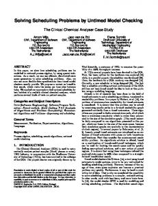
i (e.g. the main body, a link of the chassis, an axle, or a wheel) and a set of active or passive joints k (e.g. a joint connecting an axle to a wheel, or a \peristaltic" joint for modifying the length of the chassis), gure 4 illustrates. G(A) is represented using a traditional tree structure, in which the leaves represent the i and the arcs represent spatial relationships or joints. A con guration q of A is given by 6 + n parameters: six parameters (x; y; z; ; ; ) specifying the position/orientation of the main body in the reference frame of W , and n parameters specifying the values of the joints k . The terrain T is initially described using an elevation map de ned from a regular grid (x; y) expressed in the reference frame of W (such an elevation map

Motion Planning Combining Geometric and Physical Models. . . position/orientation and by force/torque parameters). In this model, the joints k of A are represented using the approach described in section 3, gure 6 illustrates. This new type of node in (A) requires to also consider the classical laws of the dynamic when propagating force and torques parameters in the network. Let ri (t) and i (t) be respectively the position and the orientation parameters at time t of a rigid body i of A. The motions of i are speci ed by the Euler/Newton equations: Ti = L_i (t) = I i (t)

Fi = mi ri (t) ;

Figure 4:

A six-wheeled vehicle on a terrain

is generally provided by a vision system). For making the collision and the contact computations possible, we have represented G(T ) as a connected set of patches.

(1)

where Fi and Ti are respectively the sums of forces and torques applied on i , Li (t) is the angular moment about the center of mass G , and I is the inertia tensor of i about the frame axes. L_ i (t) is also related to Coriolis and centrifugal terms (see [11]), but we will make the assumption that such terms are negligible (because the robot is supposed to move with a low velocity). Then, Fi and Ti can be calculated using the Euler's principle of superposition: i

i

Physical model of the vehicle. As explained in section 3, the physical model (A) of the rover A is

basically represented by a network of interacting particles. A rst way to obtain this network is to appropriately discretized the components i of A and to construct the appropriate connectors. Such an approach has already been used in [15] and in [16] for simulating the dynamic behaviour of a rover moving on a terrain. In spite of the eciency of this approach to simulate the vehicle/terrain interactions, it is not directly applicable to the motion planning problem because it is time consuming and task dependent4 . In order to reduce the computation time, we have developed an other instance of the model [5] [6] in which each sub-network associated to a rigid component of A is represented by a single node. Such a node is connected to its neighbours in the network using viscous/elastic connectors as described in section 3, but it diers from the basic particles by the fact that it obeys the laws of the physics of the solids (it is characterized in practice by

i

Fi = F d + Ti =

X Fi;j

X (G Pi;j  Fi;j ) + X

force j

i

(2)

forcej

torque k

Ti;k

(3)

where Ti;k are the torques acting on i , Pi;j are the points where the forces Fi;j are applied, G Pi;j is the vector from G to Pi;j , and  is the cross product. The term Fd includes the forces generated by the gravity and additional forces such as the viscosity of the environment. The set of forces Fi;j results from the evaluation of the physical interactions of i with the other components of (A) ?through the joints of A? and with the the involved components of (T ) ?through the wheel/ground contact interactions?. The torques Ti;k are generated by the control mechanisms (i.e. the \physical eector") associated to the wheels of A. i

i

4 On one hand, the required processing time increases

with the number of particles and of connectors. On the other hand, the processing of contact interactions requires to make use of a ne discretization of the interacting objects (and consequently to increase the number of particles).

Figure 5:

Representing a wheel of A by a set of spheres.

C. Laugier, C. Bard, M. Cherif, and A. Joukhadar tact interaction constructions described in section 3.2, gure 3 illustrates.

Physical model of the vehicle/terrain interactions. The most dicult problem to solve when deal-

Figure 6:

Modeling a 3D revolute mechanism.

Physical model of the Terrain. According to our approach (see section 3), the physical model (T ) of the terrain T is represented by a network of interacting particles. Constructing this network requires to rst determine an appropriate set of particles for representing T , and then to de ne the type of the interaction laws to associate to these particles. The rst step of the modeling process consists in converting the geometric model G(T ) of the terrain T into a set ST of spheres whose pro le approximates the surface of T (as shown in Figure 3). The sizes of the spheres which are used for constructing ST depend on the geometry of T , on the global physical characteristics of T (modeling deformable area requires more particles than rigid area ), and on the characteristics of the wheel/ground interactions to process (the sizes of the spheres used to represent T must be consistent with the number of particles and with the distribution factor used for modeling the wheels of A). In ST , each sphere (p; r) represents a particle (m; r; p), where m is a punctual mass, r is the radius of the associated non-penetration area, and p is the position of the particle. It should be noticed that this approach allows the representation of an hilly terrain using a reasonable number of elements, since the selected particles are not uniformely distributed onto the surface of T . The next step of the modeling process consists in connecting the previous particles using appropriate interaction connectors. Cohesion properties are obtained using spring/damper connectors, and surface-surface interaction characteristics are modeled using the con-

ing with a vehicle moving on a terrain, is to de ne realistic vehicle/terrain interaction laws. In our approach, such interaction laws are modeled using the basic contact interaction constructions described in section 3.2. But, the ability of the model to represent as accurately as possible the wheel/ground interactions depends on two criteria: the distribution of the contact points and the type of the surface-surface interactions to be considered. Thanks to our representation of (A) and of (T ), the distribution of the wheel/ground contact points can easily been determined using a fast distance computation algorithm involving a structured set of spheres [13]: these spheres represents the pairs (particle, non-penetration area) which model the wheels of A and the terrain T . In order to make the contact interaction computation possible, a set of elementary particles is distributed onto the contact area de ned by the contact points (see gure 3). The number of particles involved in this representation depends on both the size of the contact area and the accurancy the model. As explained in section 3.2, the surface-surface interactions are processed using two types of constructions: a viscoos-elastic law associated to a non-penetration threshold, and a surface adherence law that produces sliding and gripping eects. In order to process dry friction phenomena, we also make use of the nite state automaton described in gure 2.

4.2 Motion Planning Instanciation of the \Explore & Move" approach. As mentioned in 2.1, the problem to solve is

to nd a \safe" and \executable" motion ?(qstart ; qgoal ) allowing to move the rover A from a con guration qstart to a given con guration qgoal , while respecting a set of geometric/kinematic and of dynamic constraints COg and COd . Our approach to solve this problem is to apply an \Explore & Move" strategy. The \explore" step is executed using a discrete graph search strategy operating on the geometric model G(W ) of the

Motion Planning Combining Geometric and Physical Models. . . task; the \move" step is performed using a continuous motion generation technique operating on the physical model (W ) of the task. The \explore" function is applied at each planning step to determine a ranked set of potentially reacheable safe con gurations of A. These con gurations are then considered as the next subgoals to try to reach using the \move" function. In case of failure of the motion generation step, the system backtracks in order to process an unexplored solution. Let q be a con guration5 of A, and q~ = (x; y; ) be the 2D position/orientation parameters of q. A safe con guration of A is a con guration which satis es the following constraints COg: the wheels of A are in contact with the terrain, there is no collision between A and T , and some basic static equilibrium conditions are satis ed (no tip-over and non slidding geometric criteria). A safe con guration q of A is called a \stable placement" P (~q ) of A, where q~ represents the 2D position/orientation parameters of q. Because of the presence of the constraints COg , there exists obvious inter- dependencies between the parameters of a stable placement P (~q). This property allows us to reduce the dimension of the search space when searching for stable placements of A [4]: given a sub-con guration q~ = (x; y; ) of A, it is possible to compute the other con guration parameters of q which veri es the constraints COg . The related computation is performed by an iterative algorithm called the \placement algorithm". The basic idea in this algorithm is to simulate the falling of A onto the terrain T , at the 2D position/orientation speci ed by (x; y; ). This can be done by minimizing a \potential energy function" including a gravity term (applied to each component of A) and a spring energy term (applied to each wheel/axle joint), under a set of constraints expressing the fact that the contact points must stay on the surface of the ground (see [4] for more details). It should be noticed that this formulation of stability is based on simple geometric criteria, and that it does not guarantee the real stabil5 It has been shown in section 4.1 that a con guration

of the rover involves 6+ n parameters representing respectively the position/orientation of the main body in the 3D space and the joints parameters of the mechanical structure of A.

ity of A. It is the purpose of the next planning step to evaluate more complete stability criteria (see below).

The \Explore" function. A practical consequence of the previous property, is to make it possible to apply the discrete search strategy of the \Explore" function onto the subspace Csearch de ned by q~ ?i.e. the con guration space E (x; y; )?. This approach has already been used in [25]. It basically consists in applying an A algorithm to nd a near-optimal path in an incrementally generated graph G representing the explored con gurations of Csearch . Let q~i be the current subcon gurations of A in Csearch . The associated complete con guration of A in CA is given by the \placement" relation qi = P (~qi ), where P (~qi ) is computed using the previous \placement algorithm". Then, the expansion of the node Ni 2 G associated to q~i is obtained by evaluating a cost function and by applying a simple control u during a xed period of time
T . In the current implementation, the cost function estimates the length of the generated trajectory and the control u de nes 8 types of motion: 3 forward movements satisfying the non-holonomic constraints of A (left turn, straight, and right turn), 3 similar backward movements, and 2 \pure turns" (left and right) executed without moving A in the forward or in the backward direction (such turns are executed by applying appropriate controls onto the right and left wheels of A). The successors of q~i obtained using this technique are considered as candidates for potential stable placements of A, and only the successors which generates stable placements are stored into the ranked list which is considered for the next planning step. Let i be the best successor (according to the cost funcq~next tion) of q~i . The next planning step (i.e. the \Move" step) consists in trying to generate a continuous motion i = P (~qnext i ) allowing A to move from qi = P (~qi ) to qnext (see below). The \Move" function. The purpose of this motion generation step is to check for the existence of an exei , i.e. cutable motion allowing A to move from qi to qnext a motion which veri es the kinematic/dynamic constraints COd of the task (i.e. the kinematic/dynamic constraints of A, the constraints imposed by the ve-

C. Laugier, C. Bard, M. Cherif, and A. Joukhadar hicle/terrain interactions, and the constraints coming from the applied control strategy). Solving this problem requires to cope with dierential equations involving position, velocity and acceleration terms, and consequently to formulate the problem into the state-space STA of A. As it has already been shown in section 4.1, this can be done using our physical model (A; T ) of the task. But the main diculty which remain to overcome is to nd an appropriate way to generate a motion which allows A to move towards the next subi . Let t be the time incregoal represented by qnext ment of the motion generation process (t =
T=p), si be the state of A corresponding to the con guration qi , and let si (nt) be the state of A obtained after having applied n elementary motion step from si (i.e. after having applied a sequence of n controls on the \physical eectors" of (A)). Determining the required sequence of controls to apply to A can be done by executing an iterative algorithm involving two complementary functions: a function which hypothesizes a nominal sub-path ?ik between the current sub- con guration q~(nt) and the next sub-goal represented by i , and a function which tracks ?i while processq~next k ing the physical vehicle/terrain interactions, gure 7 illustrates. In the current implementation of the algorithm, ?ik is constructed using a technique derived from the Dubins approach [7]. Then, the obtained sub-path is a smooth curve made of straight line segments and of circular arcs (the choice of the gyration radius to apply at a given step of the algorithm depends on the length of the involved path6 and on the mechanical characteristics of A, see [6]). The tracking function operate on the model (A; T ). It takes as input the velocity controls applied on each controlled wheel during a time increment t. These controls are computed from the linear and steering speeds which are associated to the reference point of A when moving on ?ik . They are converted into a set of torques u(t) to apply to the \physical eectors" of 6 If this length is large enough, the velocities of the con-

trolled wheels are positive; otherwise, the velocities of the opposite controlled wheels have opposite signs and the vehicle will skid and use more energy to execute the motion.

(A), in order to be processed by the motion generator (see section 3.2). Since the motion generation step integrates physical phenomena like sliding or skidding, the state s?i (nt) of A obtained after having applied n successive controls may be dierent from the nominal state si (nt). The processed motion generation step will be considered as a failure when the sub-con guration q~i? (nt) is too far from its nominal value qi (nt). The previous algorithm is iterated until the neighbourhood of sinext is reached or until a failure is detected (see gure 7).

Figure 7:

The motion generation scheme.

5 The dextrous grasping problem 5.1 Task modeling As it has already been mentioned in section 2, our motion planning approach requires to combine geometric and physical models. It is the purpose of this section to describe the models which have been used to solve the dextrous grasping problem.

Geometric/kinematic models. Let G(A) and G(O) be respectively the geometric/kinematic models of the hand A and of the object O to be grasped. G(A)

is represented as an articulated object having 9 revolute joints for moving the ngers and 6 degrees of freedom for positioning the hand in the 3D space. This model is constructed using classical CAD models, and a con guration q of A is characterized by 15 parameters: six parameters (x; y; z; ; ; ) specifying the position/orientation of the hand in the reference frame of W , and 9 parameters specifying the values of the nger joints.

Motion Planning Combining Geometric and Physical Models. . . The object O is initially represented by a 3D occupancy grid which is either obtained by a vision reconstruction process or derived from a classical CAD model. For the purpose of the shape analysis process on which the \hand preshaping" step relies, G(O) has been converted into an octree representation (see [2]).

Physical model of the hand/object system. Ac-

cording to our approach (see section 3), the physical model (A; O) of the hand/object system is represented by a network of interacting particles. Constructing this network requires to rst determine an appropriate set of particles for representing A and O, and then to de ne the type of the interaction laws to associate to these particles. The rst step of the modeling process consists in converting the geometric models of G(O) and of the rigid components of G(A) into sets ST i of spheres whose pro les approximate the shapes of the associated components. As in the case of the rover application (see section 4.1), the sizes of the spheres which are used for constructing the sets STi depend on both geometric and physical criteria (shape, size, deformability factor, hand/object interaction characteristics). Each sphere (p; r) 2 ST i represents a particle (m; r; p), where m is a punctual mass, r is the radius of the associated nonpenetration area, and p is the position of the particle. The next step of the modeling process consists in connecting the previous particles using appropriate interaction connectors. Cohesion properties are obtained using spring/damper connectors, revolute joints are modeled by appropriately combining linear and torsion spring/damper connectors, and surface-surface interactions are characterized using the basic contact interaction constructions (see section 3.2). In this model, external forces are generated by the gravity, by the hand/object interactions, and by the forces/torques produced by the control mechanisms (i.e. the \physical eectors") which are associated to the nger joints. As we will see in the next section, these control mechanisms are modeled using appropriate sets of linear spring/damper connectors (the global characteristics of the associated network depend on the type of task to perform).

5.2 Motion planning Instantiation of the \Explore & Move" approach. As mentioned in 2.1, the problem to solve is

to nd a \safe" and "executable" motion for the robot hand A, starting from a given con guration qstart and ending at a partially speci ed goal con guration qgoal representing a \stable grasp" (i.e. a hand/object con guration which is accessible to the hand and which involves grasping forces allowing the robot to robustly maintain the object into the hand). qgoal is generally expressed in terms of contact relations involving features of the robot hand and of the object to be grasped. The rst step of the planning process (the \Explore" step) is to determine qgoal using an appropriate discrete search strategy operating upon the geometric model G(W ) of the task. In our approach, a partially speci ed goal con guration qgoal is represented by a \hand preshape" P which characterizes an in nite set of functionally equivalent grasps (see below). The second step of the planning process consists in searching for a particular stable grasp, by generating appropriate motion strategies constrained by both the selected \hand preshape" P and the hand/object physical interactions. This planning step is performed using the \move" function. In case of failure of the motion generation step (i.e. no stable grasp has been found), the system backtracks in order to process an unexplored solution represented by a new \hand preshape".

Hand preshaping using an appropriate \Explore" function. Because of the high dimension of

the hand con guration space CA , a classical exhaustive analysis of the set of possible grasp con gurations is not applicable when dealing with a dextrous hand. This is why we have chosen to apply another approach motivated by studies of human grasping: the human hand \preshapes" to t an object's form while reaching for it, before selecting a particular grasp using tactile and force feedback during grasp closure. Consequently, a \hand preshape" represents a class of hand con gurations from which the nal grasp is chosen. In this approach, the \hand preshaping" step relies on a taskoriented exploration of a subset of CA , and the grasp selection step makes use of a reactive motion genera-

C. Laugier, C. Bard, M. Cherif, and A. Joukhadar tor. The task-oriented exploration of CA is performed in our system using two complementary steps: (1) construct an appropriate task-oriented model of O which cleanly represents the object proportions and the accessibility relations, and (2) select a preshape P among the obtained set of candidates. An interesting property of this approach is to drastically reduce the complexity of the search step, by constructing a symbolic representation of the task which combines qualitative information (global shape, protuberances, relative size of components ...) with a limited amount of quantitative data such as the center of mass or the principal dimensions. In our approach, such a representation is constructed using the concept of \elliptical cylinder" (see [2]). Then, the task-oriented model of the task is obtained using an ecient heuristic reconstruction technique that is well- adapted to the needs of grasp planning [2]: a topographic analysis of the object shape is performed by slicing the octree model G(O), and the result of this analysis is used to reconstruct O as a hierarchy of elliptical cylinders and associated approach directions, gure 8 illustrates. Once the task-oriented model has been constructed, a particular hand preshape P and its associated goal region G on G(O) is heuristically selected. This choice mainly depends on the characteristics of the task to perform. It is perform using an heuristic function which combines hand/object proportion criteria, stability criteria, and functional knowledge about grasping. For instance, a preshape P representing a class of three-digits grasps will be chosen for robustly grasping an almost spherical object whose dimensions ts with the dimensions of the hand ngers. A preshape P produced by this planning step is characterized by the following parameters [2]: the relative hand/object location which is considered as the starting point for the closure step, the approach direction for the hand, and the intended con guration and contact parameters for the ngers (i.e. the number of nger involved, the type of contact to achieve ?tip, pad, or palm?, and the relative placement of the ngers when executing the grasp operation ?opposition between the thumb and the other ngers, opposition between the three ngers ...?). It has been shown in [2] that a small number of

dierent types of preshapes are needed (for instance, only 12 types of preshapes have to considered for our three- ngered hand).

3D reconstruction of a mug as a hierarchy of elliptical cylinders ECi and their associated approach directions Dik . Each pair (ECi ; Dik ) represents a candidate for a \hand preshape". Figure 8:

Grasp determination using a \Move" function.

The purpose of this motion generation step is to check for the existence of an executable motion of A ending at a con guration q ? goal corresponding to a stable grasp of O. The constraints COd to satisfy during this motion are the kinematic/dynamic constraints of A, the constraints imposed by the hand/object interactions that must respect some given equilibrium conditions, and the constraints coming from the applied control strategy. As in the case of the rover, this problem has to be formulated in the state space STA of A for being solved. This is done using our physical model (A; O) of the task (see section 5.1). Then, the equilibrium conditions SG P(O) can easily be expressed as follows: V~ = ~0 and F~ext = ~0, where V~ is the speed of O and each F~ext is an external force applied on O (i.e. a gravity term or a force applied by a nger of A)7 . Let qi and si be respectively the hand con guration and the hand state associated to the selected preshape P . Then, the problem to solve is to generate an executable motion ?(qi ; qgoal ) of A (i.e. a motion which veri es the constraints COd ) starting at si and ending at a state sgoal characterized by the equilibrium condition SG(O). Since COd includes contact conditions imposed by P , ?(qi ; qgoal ) obviously depends on 7 Generating a force-closure grasp allowing the execution

of a task requiring to apply a force Ftask onto the object O can easily been done by introducing this new term within the expression F~ext = ~0.

P

Motion Planning Combining Geometric and Physical Models. . . index and major

(a)

LS1 thumb (b)

a control point on the object

LS1 LS2

(c)

LS1 LS3 LS2

Figure 9: De ning grasping strategies using appropriate

sets of LS relations for connecting the joints of A: (a) executing a tip contact based grasp; (b) executing a pad contact based grasp; (c) executing a palm contact based grasp.

the type of grasp to achieve: a grasp consisting in surrounding the objet with the articulated ngers will not involve the same control strategy that a tip contact based grasp. In our approach, a particular grasping strategy is achieved using an appropriate set of linear spring/damper connectors (LS connectors) for connecting the joints and the nger tips of A, gure 9 illustrates. Let (Pi ; Pj ), (; ), and (lo; l) be respectively the pair of particles to connect, the rigidity/viscosity factors, and the nal/initial length of the considered LS connector. The values to associate to these parameters depend on the type of the involved hand/object contacts (tip, pad, or palm contacts) and on the characteristics of the grasp to achieve: pairs (Pi ; Pj ) are de ned by the hand/contact characteristics, (; ) parameterizes the motion generation process, and pairs (l; l0 ) are de ned by the preshape P and by the local morphological characteristics of O. For instance, a \spherical grasp" involves an l0 value depending on the global size of O, while a \cylindrical grasp" will generates a small l0 value for the pair (index, major), and a l0 value depending on the size of O for the pair (index, thumb). Complete motion strategies can also been generated using a similar approach using a \ghost" model of the moving object for representing the goal to achieve ( gure 10 illustrates).

6 Implementation and Experiments The approach presented in this paper has been implemented on a Silicon Graphics workstation within the

(b) (a) a control particle on a nger

(c)

Figure 10: De ning motion strategies using a set of LS re-

lations for connecting the control points of the moving object A with the associated \in nite mass particles" belonging to a \ghost" of A which is located at the goal con guration: (a) A is attracted towards the selected preshape; (b) the ngers of A attract each others in order to achieve the required grasp; (c) the goal con guration of the object O attracts the hand/object system.

robot programming system ACT8 . Several experiments have been successfully processed in simulation for both the rover application and the dextrous grasping application.

The Rover Application. The rover A considered for these experiments is a non-holonomic vehicle having an articulated mechanical structure and a locomotion system composed of six motorized wheels, gure 4 illustrates. The central pair of wheels is connected to the main body of A and the two others pairs of wheels are respectively connected to the front and the rear axles of A. These axles are connected to the chassis by joints allowing roll and yaw movements, and the front and the rear links of the chassis are articulated in order to enable a \peristaltic" transformation of A. Figure 11 shows the trajectory generated by the system when only forward and backward motions respecting the non-holonomic constraints of A are allowed. Figure 12 shows the trajectory obtained when \maneuvers" are allowed (i.e. when \pure turns" that locally violate the non-holonomic constraints can be executed by A, see section 4.2). In this case, the produced maneuver is executed by applying controls having opposite signs onto the wheels of each axle; the smooth part of the trajectory is executed by applying positive controls of various magnitudes onto the wheels of each 8 The ACT system is developed and currently marketed

by the Aleph Technologies Company.

C. Laugier, C. Bard, M. Cherif, and A. Joukhadar axle. Figure 13 shows the pro les of the forces applied on the six wheels of the rover when executing the last left turn of the trajectory shown in gure 11. In these pro les, the location of the forces having a large magnitude corresponds to the place where the wheels are crossing an irregular area.

Figure 11: Trajectories executed by the main body and the six wheels of A when no maneuver is allowed.

Figure 12: Trajectories executed by the main body and

the six wheels of A when maneuvers are allowed.

The dextrous grasping application. The articulated hand A used for these experiments is composed of three ngers, where each nger has three links connected by two revolute joints, see gure 14. In the physical model (A), the links of the ngers are mod-

Figure 13: The forces applied on the wheels of the three axles of A during the execution of the last left turn of the motion shown in the previous gure.

eled by n particles connected by (n ? 1) LS relations and by (n?2) TS relations. As explained in section 5.1, the number n of particles depends on the characteristics of the task to perform (and in particular on the deformability properties to consider). In the shown experiments, only 3 particles have been used to model each rigid link of the ngers of A. Several grasping experiments have been processed with this simple hand, by considering tip or pad contacts involving various friction parameters. Figure 14 shows how a grasping operation may fail when friction forces are not sucient to generate a stable grasp. Some other experiments have also been processed using a physical model of the Salisbury hand (this model is composed of 300 particles). Despite the increasing number of particles, these experiments have shown that the motion generation process could be still performed in \real time" (i.e. a motion step is generated in less than one second).

Motion Planning Combining Geometric and Physical Models. . .

Figure 14: (A simple articulated hand trying to grasp a bar: (1) hand preshaping step; (2) rst closure step ending when

the nger/object contacts have been achieved; (3) next closure step consisting in applying the computed forces at the contact points (the object is subjected to a deformation); (4) the bar slips out of the hand because the friction forces are not sucient to generate a stable grasp.

Acknowledgment The work presented in this paper has been partly supported by the CNES (Centre National des Etudes Spatiales) through the RISP national project, the MRE (Ministere de la Recherche et de l'Espace) and by the Esprit-BRA project SECOND. It has been also partly supported by the Rh^one-Alpes Region through the IMAG/INRIA Robotics project SHARP.

References [1] B.S. Baker and S. Fortune and E. Grosse: \Stable prehension with a multi- ngered hand", IEEE Int. Conf. on Robotics and Automation, 1985, March, St Louis. [2] C. Bard , C. Laugier , C. Milesi-Bellier, J.Troccaz, B. Triggs , G. Vercelli: \Achieving dextrous grasping by integrating planning and vision based sensing", International Journal of Robotics Research. To appear in 1994. [3] M.G. Bekker: \Introduction to Terrain-Vehicle Systems", The University of Michigan Press, 1969. [4] Ch. Bellier, Ch. Laugier, B. Faverjon, \A kinematic Simulator for Motion Planning of a Mobile Robot on a Terrain", IEEE/RSJ Int. Workshop on Intelligent Robot and Systems, Yokohama, Japan, July 1993.

[5] M. Cherif, Ch. Laugier, \Using Physical Models to Plan Safe and Executable Motions for a Rover Moving on a Terrain", First Workshop on Intelligent Robot Systems, J.L.Crowley and A. Dubrowsky (Eds), Zakopane, Poland, July 1993. [6] M. Cherif, Ch. Laugier, Ch. Milesi-Bellier, B. Faverjon, \Combining Physical and Geometric Models to Plan Safe and Executable Motions for a Rover Moving on a Terrain", Third Int. Symposium on Experimental Robotics, Kyoto, Japan, October 1993. [7] L.E. Dubins, \On Curves of Minimal Length with a Constraint on Average Curvature, and with Prescribed Initial and Terminal Positions and Tangents", in American Journal of Mathematics, 79:497-516, 1957. [8] R.S. Fearing: \Implementing a force strategy for objects re-orientation", IEEE Int. Conf. on Robotics and Automation, San Francisco, April, 1986. [9] T. Fraichard and C. Laugier: \Dynamic Trajectory Planning, Path-Velocity Decomposition and Adjacent Paths", Int. Joint Conf. on Arti cial Intelligence, 1993, August, Chambery, France. [10] D. Gaw, A. Meystel, \Minimum-time Navigation of an Unmanned Mobile Robot in a 2-1/2D World

C. Laugier, C. Bard, M. Cherif, and A. Joukhadar with Obstacles", IEEE Int. Conf. on Robotics and Automation, April 1986.

[11] H. Goldstein, \Classical Mechanics", 2nd edition, Addison-Wesley, Massachusetts, 1983. [12] H. Hanafusa and H. Asada: \Stable prehension by a robot hand with elastic ngers" 7th Int. Symp. on Industrial Robots, 1977, October, Tokyo. [13] J.E. Hopcroft, J.T. Schwartz, M. Sharir, \Ecient Detection of Intersections among Spheres", Int. Journal on Robotics Research, Vol. 2, No. 4, 1983. [14] P.M. Isaacs, M.F. Cohen: \Controlling dynamic simulation with kinematic constraints, behaviour functions and inverse dynamics", Computer Graphics(SIGGRAPH'87), 21(4), July 1987. [15] S. Jimenez, A. Luciani, C. Laugier, \Physical Modeling as an Help for Planning the Motions of a Land Vehicle", IEEE/RSJ Int. Workshop on Intelligent Robot and Systems, Osaka, Japan, November 1991. [16] S. Jimenez, A. Luciani, C. Laugier, \Predicting the Dynamic Behaviour of a Planetary Vehicle Using Physical Models", IEEE/RSJ Int. Workshop on Intelligent Robot and Systems, Yokohama, Japan, July 1993. [17] J.C. Latombe, \Robot Motion Planning", Kluwer Academic Publishers, Boston, USA, 1990. [18] A. Liegeois, C. Moignard, \Minimum-time Motion Planning for Mobile Robot on Uneven Terrains", in Robotic Systems, Kluwer 1992, pp. 271-278. [19] A. Luciani and al: \An uni ed view of multiple behaviour, exibility, plasticity and fractures: balls, bubbles and agglomerates", IFIP WG 5.10 on Modeling in Computer Graphics, Springer Verlag, 1991, pp.55-74. [20] H. Maekawa: \Stable grasp and Manipulation of 3D Object by Muti ngered Hands", International Symposium on Measurement and Control in Robotics (ISMCR'92), 1992, November, Tsukuba, Japan.

[21] M.T. Mason: \Manipulator grasping and pushing operations", Massachusetts Institute of Technology, 1982, June. [22] V. Nguyen: Constructing force-closure grasps in 3D, IEEE Int. Conf. on Robotics and Automation, 1987, March/April, Raleigh. [23] Z. Shiller, J.C. Chen, \Optimal Motion Planning of Autonomous Vehicles in Three Dimensional Terrains", IEEE Int. Conf. on Robotics and Automation, May 1990. [24] Z. Shiller, Y.R. Gwo, \Dynamic Motion Planning of Autonomous Vehicles", IEEE Trans. on Robotics and Automation, vol 7, No 2, April 1991. [25] Th. Simeon, B. Dacre Wright, \A Practical Motion Planner for All-terrain Mobile Robots", IEEE/RSJ Int. Workshop on Intelligent Robot and Systems, Yokohama, Japan, July 1993. [26] D. Terzopoulos, J. Platt, A. Barr, K. Fleischer: \Elastically deformable models", Computer Graphics, 21(4), July 1987. [27] D. Terzopoulos, K. Fleischer: \Modeling inelastic deformations: Visco-elasticity, plasticity, fracture", Computer Graphics, 22(4), August 1988. [28] J. Pertin-Troccaz: \Grasping: a state of the art", The Robotics Review, MIT Press, Spring, 1989.