Solving Decision Problems by Distributed Decomposition and Delegation. ---. Foundations of a Theory and its Application within a. Normative Group Decision ...
Solving Decision Problems by Distributed Decomposition and Delegation --Foundations of a Theory and its Application within a Normative Group Decision Support System framework Oliver Wendt, Peter Rittgen and Wolfgang Koenig, Frankfurt University, Germany email {wendt, rittgen, koenig}@wiwi.uni-frankfurt.de
1. Introduction Imagine being the manager of a project that aims to reorganize and optimize the distribution logistics of your company. Your project team consists of several members, each member being an expert on a different domain. Imagine furthermore, your team members would be geographically dispersed. We assume that the team members are linked by phone, fax, or electronic mail. Moreover, all team members use a tool like Lotus Notes to structure and access their documents. Still, you and your team members require the use of a normative group decision support system that
r r
provides imperatives on how to logically structure the decision problem and the solution process, and provides optimization tools.
As we are talking about so-called unstructured decision problems, we cannot set up an imperative to optimize the decision object (e.g. "You have to buy this particular part of the logistics services from an outside vendor!"). We do not even know which kind of partitioning of the problem is most suitable. Instead, we only can try to optimize the planning and decision process in a group of collaborators (which then, when being performed, may lead to optimal solutions of the decision objects). We set up on the paradigm that the solution of an unstructured decision problem is created by repeatedly decomposing the original decision problem and its components into less complex / unstructured components until we reach a sub-problem which in fact is structured (i.e. there is an imperative available on how to solve this particular sub-problem). So, integrating the solutions bottom up along the decomposition graph yields the solution of the originally unstructured problem. However, the decomposition structure of an unstructured problem is not trivial. We introduce the so-called ANDORI language which enables users to describe both AND and OR decomposition of an original problem as well as the description of so-called information edges between ANDed components of an original problem (e.g. precedence structures, see chapter 2).
-- 2 -The process of structuring and solving unstructured decision problems occurs facing a tradeoff between
r r
trying to find an optimal solution for the decision object (in our case for example reducing the logistics costs by buying appropriate services from outside vendors), and trying to minimize the search costs for a yet unknown result (in our case for example hiring a consultant to buy special expertise in logistics).
In particular, we run into a modeling problem as we are working in a discrete world and modeling all possible decompositions of a problem seems to be far too expensive. Instead, we need a technique that enables us to selectively build up a problem decomposition graph, top down, directed towards an optimal decomposition path. Thus, we develop a so-called modeling cost theory (chapter 3) that integrates both the benefits of a particular problem decomposition on the level of the decision object and the modeling costs that are necessary to realize this solution. Using particular estimators for both classes of costs, our normative group decision support system identifies the node in the decomposition graph which has to be expanded next (see chapter 4). Moreover, this decomposition graph also acts as a basis to optimise the delegation of the decomposition of sub-problems. There are two extreme approaches to coordinate delegates during the distributed process of decomposition: Either there is no coordination (i.e. all possible nodes for further decomposition are modeled in parallel, without for example learning particular structures of the global problem or its solution from other decomposers). Or we perform a centralized coordination (causing high communication costs and requiring a large central throughput). By evaluating the trade-off between the expected number of nodes to be expanded in the course of problem decomposition (in fact the modeling costs of all of these nodes) an the coordination costs, we may determine an optimal distribution degree of the problem decomposition (see chapter 5). All these tasks of structuring yet unstructured decision problems belong to phase 1 of the decision process which terminates when a decomposition graph representing a valid solution to the problem is found. In phase 2 the normative group decision support system supports the integration of the sub-solutions from the different collaborators and, in case of conflicts, suggests a revision of the original problem decomposition. After completion, in phase 3 the normative group decision support system controls the distributed execution of the decentralized problem solution process. However, in this present article we concentrate only on phase 1 of the decision process, the distributed decomposition and delegation and its support by a normative group decision support system which is called "Distributed Reasoning Support System (DRSS)".
-- 3 -2. Syntax and Semantics of ANDORI graphs We further specify our logistics case: Due to the fact that you (the project manager) received several offers of third-party forwarders that sound reasonable to you, you consider your logistics problem being a MAKE-OR-BUY problem (refer to fig. 1). You could either go on providing the distribution logistics all by yourself or buy a packaged service from one of those external forwarders 1. make or buy
MAKE
DIS
I plans
BUY
PHY
Figure 1: simple ANDORI graph The relation between the MAKE-OR-BUY problem and its two sub-problems is called an OR relation, due to the fact that the alternatives are mutually exclusive, which means that you will never implement both of the two partial plans, MAKE and BUY, to the real world, although you have to solve both of the two planning problems in order to find out which alternative is the one with the lowest cost. In case you decided to reason about the MAKE alternative first, you may want to think of distribution logistics as some sort of compound of physical logistics activities, in the sense of driving from customer A to customer B or loading the cargo into a truck, and dispositive logistics, which consist of planning the allocation of a given set of cargo to the available trucks and planning the routing for each of them. The relation between the MAKE problem and its two sub-problems is quite different to the one discussed on top level: It is not enough to just implement the solution of either one of the two sub-problems, you rather have to solve them both in order to find an appropriate plan for the MAKE problem. For this reason, the relation is called an AND relation and is denoted by an arc connecting the two vertical edges. The sub-problems of an AND decomposition may have functional dependencies denoted by information edges. Figure 1 shows a precedence relation between two nodes: in order to execute the physical logistics, the dispositve logistics department has to provide the plans for routing your trucks2. The plan itself is passed from the DIS node to the PHY node (Iplan). 1
Of course, this is a simplification, since it might be possible to find possible "mixtures" of making some services and buying some others.
2
It has to be noted here that the information edge I states a precedence relation constraining the execution of the partial plans and not the planning process itself. Planning may still be performed in parallel, although when designing the organization of the physical logistics we have to design a "business
-- 4 -Other types of functional dependencies are discussed in [Wendt 93]. So, the domain independent problem statement language ANDORI extends the known AND/OR graphs [Pearl 84] by the so-called information edges (I edges), hence its name. Due to time restrictions or a lack of competence you decide to consult (internal or external) experts and delegate the partial tasks to them. The three partial tasks are: DIS: PHY: BUY:
Find the best organization for planning our distribution logistics; evaluate the cost of implementing this organization and using it for the next five years. Find the best organization for physically distributing goods to our customers, evaluate the cost of implementing this organization and using it for the next five years. Find the best external forwarder by evaluating the quality and cost of their service for the next five years.
None of these problems is trivial in the sense that a solution might be given without further investigations. Unfortunately, the cost of further investigations into the BUY branch of the search tree will be sunk when it finally turns out that the MAKE branch leads to a superior solution (and vice versa). To constrain the search and modeling cost, we need an estimation telling us which parts of the global decomposition graph lead to an optimal solution and which cost this modeling brings about. Formally we speak of identifying the correct sub-graph in the decomposition hierarchy which rewards modeling (refer to chapter 4.5). Formally, an ANDORI graph is a tuple (V, EA, EO, EI, I, F) consisting of a set of vertices V, also called nodes, a set of AND edges EA, a set of OR edges EO, a set of information flow edges EI, a set of information flows I associated with the corresponding edges in EI, and a set of goal functions F associated with each vertex. The tuple elements are defined as follows: V:
a set of vertices (or nodes) representing problems or solutions in case that all sub-problems have been solved
2V :
the set of all sub-sets of V, i.e. collections of problems
EA ⊂ V × 2 V :
a set of AND edges, the first element of each pair being the parent vertex (super-problem), and the second being a set of child vertices (sub-problems)
EO ⊂ V × 2 V :
a set of OR edges with tuple elements as in EA
EI ⊂ V × V :
a set of directed I edges (information edges), the first element of each pair denoting the source vertex, and the second denoting the destination of the information flow
process" which is capable to execute any possible plan which might be provided by the DIS process in the excecution phase.
-- 5 -I = {I i i ∈ E I }:
a set of information flows (one for each I edge)
I i ∈ 2 D × B:
the first element of the pair is a set of variables (data flow), the second is a boolean function of this set (control flow)
D:
the set of all variables (data)
{
}
B = Θ Θ:2 D → {true, false}
the set of all boolean functions on the set of all variables F = { f i i ∈V }:
a goal function fi for each vertex i which has to be minimized3
Restrictions: ∀( p, C ) ∈ E A ∪ EO : p ∉C ∧ C ≥ 2:
no parent is its own child, and at least two children are required (no renaming)
∀(s, d ) ∈ EI : ∃(p, C ) ∈ EA :{s, d} ⊆ C:
information can only flow between the ANDed children of a node4
∀( p, C ) ∈ E A ∪ E O : f p = Θ({ f c c ∈ C}):
aggregation of goal functions along the hierarchy5
For the example of figure 1 we have: V = {make _ or _ buy, MAKE, BUY , DIS, PHY } EA = {(MAKE, {DIS, PHY })}, EI = {( DIS, PHY )},
{
{
EO =
}
I = I(DIS , PHY ) , I(DIS , PHY ) = I plans
F = fmake _ or _ buy , fMAKE , fBUY , fDIS , fPHY fmake _ or _ buy = min( fMAKE , fBUY ),
3
{(make_ or _ buy,{make, buy})}
}
fMAKE = fDIS + fPHY
We do not have to consider maximization problems explicitly, since maximization of a term f can be accomplished by minimizing -f.
4
Since OR nodes represent a choice between mutually exclusive alternatives, information cannot flow between them.
5
This restriction forces the goal function fp of the parent node p to be expressed by some arbitrary function Θ on the goal functions of its children. It ensures that the decomposition of a parent node is complete in the sense that the quality of the solution of p does not depend on anything else but the solution of its sub-problems.
-- 6 -Semantically, the ANDORI framework adopts the state space view of problems and problem solving, i.e. a problem P may be defined by a tuple (X, I, H, f, O) consisting of the set of all states X (the state space), a set of initial states I, a set of hard constraints H, a goal function f defined on all states complying with all hard constraints in H and a set of set of operators O transforming states (going from one state to another). Imagine the state space X = X1 × X 2 × × X n : to be the set of all possible combinations of action variables X1..Xn the
L
decision maker can control6. Initially the "world" is in a state x ∈ X . You may change this state x into a state x' by applying an operator o: X → X to the initial state. By applying a sequence of operators o ∈ O to the state x and its transformations you try to reach some optimal goal state x*, the solution of your problem P. What are the properties of this goal state x*? First of all, it must not violate any hard constraint hi ∈ H . Each of these hard constraints can be represented by a boolean function h: X → {true, false}. Let us define the solution space S ⊆ X to be the subset of all states in X,
{
which do not violate any of the hard constraints, i.e. S = x ∈ X h1 ( x ),
L, h ( x)}. Our final goal
is to find an x* ∈ S for which the value of our goal (cost) function f : S →
k
R is minimized.
We introduce a set I of initial states here (instead of just one initial state) to enable the description and solution of a problem class. The sequence of operators that solves the instance of the problem class associated with a specific initial state x ∈ I is a function of that state x. For example, our planning task PHY in the Make-or-buy example is of this type, since we do not know the plans delivered by DIS in advance. Therefore, the solution to PHY is a "program" capable to process all possible results of DIS correctly. In the light of these definitions, the semantics of an OR decomposition can be outlined as follows: The total solution space S for the given problem P is partitioned into p sets of alternatives that can be explored separately7. The solution to P is the one alternative with the minimal cost f. The following restrictions have to hold:
L
S = S1 ∪ S2 ∪ ∪ S p :
( )
( ( ) L, f (x )):
x S* = x S*i : fS x S*i = min fS1 x S*1 ,
Sp
* Sp
the total solution space S of the parent node is covered by its children the best alternative xS* of the parent problem is identical to the best solution xS*i over all sub-spaces Si.
6
In this paper we assume certainty about the environmental variables, i.e. we do not cope with uncertainty here, which would change the focus from "minimizing the cost f of the solution" to "minimizing the expected cost".
7
Note that in the case of unstructured problems (like our make-or-buy example) we do not know the solution space S in advance, i.e. we cannot enumerate the nodes of our search tree. Nevertheless, we are able to partition this unknown set S into smaller subsets S1 and S2, namely the set of all MAKE alternatives and the set of all BUY alternatives.
-- 7 --
L
Regarding the semantics of an AND decomposition, we define the following: The action variables X1 , X2 , , Xn are partitioned into q different groups in such a way that the following equations should8 hold true:
L
S = S1 × S2 × × Sq :
((
all variables are accounted for exactly once
L )) = min({f ( x) x ∈ S}):
fS x S*1 , x S*2 , , x S*q
S
the combination of the partial maxima is also a global maximum for the parent problem
The principal advantage of ANDORI graphs over AND/OR graphs is that the I edges enable the modeling of information flow between actors, thus explicating the functional dependencies between partial sub-problems and their respective solutions. These dependencies are hidden in pure AND/OR graphs, and can therefore not be dealt with. Different types of dependencies exist: Temporal precedence:
The most frequent dependency. Task A has to be performed before task B (see figure 1).
Conditional sequence:
The execution of task B depends on the result of task A.
Conditional loop:
A sequence of tasks is iterated depending on a loop condition.
Based on interpreting the information edge as the joint data and control flow we have developed an algorithm9 for detecting latent parallelism, which is described in [Wendt 93]. This algorithm supports the decision maker(s) when deciding which parts of the ANDORI graph may be delegated to independent problem solvers and where such a distributed problem solving leads to high coordination costs when integrating the (potentially incompatible) results. We have now completed the description of the ANDORI language itself. The following chapter addresses the search for a solution in ANDORI graphs.
8
In many cases it may be advantageous to violate those constraints in order to derive partial models that are easier to solve. This is "paid for" by higher costs for integrating the partial solutions.
9
This algorithm is based on a data flow analysis as used in compiler theory [Aho 84].
-- 8 -3. Modeling cost theory as a guide to optimal search in problem decomposition hierarchies Consider again the MAKE branch of our logistics problem. Different domains of the economic sciences have developed different methods of determining an optimal organization, for example Cost Accounting or Operations Research. You may either set up complex combinatorial optimization models for tour planning and simulate their results in order to get a cost figure or you may apply simple heuristic methods (for example take last years cost of your logistics department as a budget for this year's activities). Both methods solve the given task but differ in the solution process as well as in the solution quality. The simple heuristic only requires modeling a small part of the global problem and aiming for an "acceptable" solution, which can be handled much easier. But the heuristic cannot guarantee that the optimal solution of the global problem is reached. On the contrary, optimization methods lead to the optimum, but usually require a higher amount of modeling and computation time. Generally speaking, the more you spend on modeling, the higher the quality of the solution and the lower the cost of the execution. Between these two poles, various methods are known which provide a specific mixture of modeling simplicity, solution speed, quality of the solution and distance of the modeled problem to the original problem. The theory of complexity may be used to compare the computational resources needed for two algorithms A and B, solving the same problem to optimality. But it does not help us in the case of an unstructured problem, where we try to achieve the "best compromise" between the quality of the solution (in our case e.g. the number of miles of a round-trip) and the cost invested for obtaining this solution. Using a modeling cost theoretic approach [Koenig 94] we get: Minimize: C = Cf + Cm, Cf Cm
being the cost of executing the solution found in the decision process being the cost of modeling and solving the problem.
The cost of modeling includes for example:
r r r r r
the cost of learning a domain terminology of a solution method, the cost of learning and applying this method, the associated hardware and software cost, the cost of convincing the members of the project team of the quality of this method, and, the cost of assuring the quality of the correct application of the method.
While for example the cost of learning a new method is usually paid only once, the cost of applying this method to a problem as well as the opportunity cost incurred by applying a suboptimal method have to be viewed as a sum of discounted cash flows occurring over a long period of time.
-- 9 --
How can we apply these criteria in order to develop guidelines for distributed problem solving in the ANDORI framework? To answer this question, let us focus on a search in pure OR-trees from now on10.
4. Economic search: Optimally trading off solution quality and planning cost When we constructed our ANDORI tree for the logistics example (Fig. 1), it was clear that the bottom nodes of this tree are not leaf nodes in the sense that they represent "trivial problems". Therefore, in order to solve our global problem, planning has to proceed by "expanding" one of the bottom nodes, i.e. transforming it into simpler sub-problems. But, which of the nodes should we expand first? We are looking for a function f (i ∈V ) , telling us the cost of the optimal leaf node, that an expansion of node i will eventually reveal. Unfortunately, we may only estimate the true cost value f (i ∈V ) by an estimator f ' (i ∈ V ) . It can be shown [Pearl 84, p. 75] that performing a best-first search in an OR tree, which means to always expand the node i with the lowest cost estimator f ' (i ∈ V ) leads to an optimal solution of the problem if the estimator is optimistic, i.e. f ' (i) ≤ f (i ) ∀i ∈V . We have to continue our expansion process until the following condition is true: The node i with the lowest cost estimator is a leaf node. For leaf nodes f ' (i) = f (i ) and due to the optimism of the estimator f ' we therefore know that all other branches of our tree could only yield solutions with higher costs than f (i) . This in turn guarantees that i is one of the optimal solutions to our problem, i.e. it does not pay to continue the search process. Unfortunately, the total number of nodes that we will have to expand depends on the quality of our cost estimator f ' . If it is too optimistic (just imagine f ' (i ) = 0 ∀i ∈ V ), almost every node of the search tree will have to be expanded in order to guarantee the optimality of a solution. In contrast, we reduce the number of nodes to be expanded by minimizing the difference between f ' (i ) and f (i) . On the other hand, when we observe complex decision processes in organizations, we find people rather looking for realistic than for optimistic cost estimates for a given subset of all possible actions. This phenomenon can easily be explained by the existence of modeling costs: The best-first search described above just focuses on how to obtain an optimal solution in a minimal number of search steps. In contrast, when we encounter substantial modeling costs, it may be advantageous to give up the requirement of finding an optimal plan in order to reduce the cost of planning.
10
The extension of this search to general AND/OR graphs or ANDORI graphs is much more involved but does not add new insight to the findings presented here. The reader interested in the details of those extensions is referred to [Wendt 93].
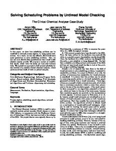
-- 10 -Basically, we have to replace our old cost estimator f ' (i ) , which was just representing the estimated cost of executing the best plan obtainable by pursuing alternative i by a new one f ' ' (i ) = f ' (i ) + m' (i ) that also accounts for the estimated modeling cost m' (i ) that we will have to pay in order to find this solution. A central finding of our modeling cost theory is, that (contrary to the results for f ' (i ) in the case of no modeling costs) it is not advisable to use an optimistic estimator f ' ' (i) . While in the case of no search cost you could easily "backtrack" to another, more promising branch of the search tree, once your initial cost estimation had turned out to be too optimistic, the exploration of a misleading branch of the search tree will now cause search costs that are sunk. That means that search errors cannot be undone anymore without losing invested modeling and search costs. Since we cannot use an optimistic estimator alone in the presence of search costs, we assume that it is possible11 to bind the costs from above, too, i.e. for every node i of our search tree we estimate the plan execution costs to be within the interval f '(i ); f '(i) and the cost of planning
[
[
]
]
to be bound within m'(i ); m'(i ) . Graphically we may represent this available cost information on each node by a box as in figure 2. 300
(20;300)
node 1 250
(25;250)
node 2 200 f'(i)
150
100
(10;100)
50 (15;20)
0 0
5
10
15
20
25
30
m'(i)
Figure 2:
Characterization of two possible branches of the search tree
Which of the two nodes given in fig. 2 should we expand? For every point (m' (i); f ' (i)) within the box i there is a probability density p(m' (i ); f ' (i )) indicating the chance that the search for a leaf node beneath node i will eventually yield a leaf of cost f ' (i ) after investing m'(i ) for further planning activities. The expected total cost f ' ' (i) for continuing the search with node i may be calculated to be
11
In practice, you will frequently hear people estimating costs to be "within the range of X and Y". We therefore believe this to be a valid assumption.
-- 11 --
m' ( i ) f ' ( i )
∫ ∫ p(m; f ) ⋅ (m + f )⋅ df ⋅ dm
f ' ' (i ) =
∀i ∈ V .
m' ( i ) f ' ( i )
As long as we do not have any further information on the probability density within the boxes, we will assume a uniform distribution. In this case, we may simply determine the center of gravity for each box and calculate the total cost for this point. With this method we get a total expected cost of 215 for node 1 and a cost of 155 for node 2. We therefore decide to expand node 2. Let us assume that node 2 decomposes into two new nodes, namely node 21 and node 22. One of them (node 21) being a leaf node of cost 170 and the second one having the upper and lower cost bounds illustrated in figure 3. As we see, the expanded node 2 itself disappeared, but the alternative node 1 is still available. The leaf node 21 is just a point (0; 170) on the y-axis, since it provides a plan of sure cost 170 which does not require any further modeling. (20;300)
300
node 1 (13;250)
250
node 22
node 21 200 f'(i)
150
f''(i)=170 (10;100)
100 (5;90)
50
0 0
5
10
15
20
25
30
m'(i)
Figure 3:
Should there be any further planning activities ?
How to proceed from this situation? Should we stop planning and execute the solution provided by node 21? When we calculate the centers of gravity for the two yet unexpanded nodes we obtain expected costs of 215 for node 1 (as before) and 179 for node 22. We see, that the centers of gravity for both boxes lie above the line through all points of total cost f ' ' (i) =170. Although these results recommend to stop the search, we should not do so. In fact, the old way of calculating the expected cost for the two unexpanded nodes is no longer appropriate as soon as we have an executable plan available! Since we can always use this plan with costs of 170 as a "backup solution" we do not have to fear obtaining a solution worse than 170 by continuing the search. Consider an expansion of node 22: Should we decide to expand this node and after a total investment of 10 units of search cost end up with a plan of execution cost 200, we will of course discard this plan and use plan 21 instead. Graphically this means,
-- 12 -that once a solution of cost b is obtained, the probability density above the dashed line "shrinks down" onto this line for every unexpanded node. Formally, this means
∫ ∫ p(m; f ) ⋅ (m + min( f ; b))⋅ df ⋅ dm
m' ( i ) f ' ( i )
f ' ' (i ) =
∀i ∈ V .
m' ( i ) f ' ( i )
Using this rationale to recalculate the expected costs for the two yet unexpanded nodes, we obtain expected total cost of 173 for node 1 and 159 for node 22. Thus it is indeed advisable to expand node 22 although there is a 50% chance of not finding any solution better than 170 by doing so. The expansion should be stopped when all unexpanded nodes yield estimates above the cost bound b .
5. Distribution of decomposition tasks to cooperating agents When discussing the motivation for our ANDORI graphs, we assumed that each node of the graph can be assigned to some actor who creates a plan to solve this partial problem. Apart from the information edges which indicate dependencies, the actors do not require any coordination before they return their (partial) results to the delegator. As we have seen in the last chapter, this totally parallel processing of the problem decomposition graph would lead to a rather inefficient search when the ANDORI graph contains many OR nodes. We therefore explored different mechanisms for coordinating such a parallel search. Totally distributed processing with no coordination (NC) Just imagine that you may dispose of n actors helping you with your task of searching an OR tree for the best solution to a given problem. Once you have expanded the top node of a pure OR tree, you may distribute the work of further exploring the m sub-problems to the n actors. Even if we assume that m=n and every actor receives one "chunk" of the solution space S, it will eventually turn out that n-1 of the n agents did explore the "wrong regions" of the solution space instead of helping the one agent (who got the right region assigned) to explore his region faster. Centralized coordination (CC) The other extreme would be to require each of the n agents just to expand the one assigned node and immediately return all child nodes to you. After you have collected all child nodes from all agents you sort them by their cost estimator f ' ' (i) and distribute the n best nodes of your list to the n actors in order to ask them again for just one expansion. As you may imagine, this model will reduce the total number of node expansions significantly, compared to the NC model. On the other hand, there will be a huge communication load compared to the NC model. Especially, the central coordinator becomes a bottleneck, when the number of available actors increases, thereby restricting the possible speedup [Finkel 87].
-- 13 -Distributed Coordination (DC) We therefore explored a distributed coordination model. After the initial distribution of m ≥ n nodes to the n agents there is no global coordination anymore until the point in time when all n agents have terminated their search. But in contrast to the NC model, each of the n processors "informs" the other agents of the intermediate results. To do this, we simply introduce a node distribution step after the node expansion step. This means that after all n actors have expanded the best node of their "private" list of yet unexpanded nodes, the new list gets resorted by increasing values of the estimator f ' ' (i) . Now the actor distributes the best nodes from its list of unexpanded nodes (up to a fraction d of the total number of nodes on this list) to other actors by deleting the nodes from their own list and "mailing" them to a different actor. The receiving actor for the transferred work could either be chosen randomly among all "coworkers" or by a predefined "distribution topology" 12. Our empirical tests with the different distribution models yielded the following results 13:
r
r r r r 12
Whether parallel search "pays off" strongly depends on the quality of the estimator f ' ' (i) . When its quality is poor (i.e. it is too optimistic) and modeling costs are low, many branches of the search tree eventually have to be explored. A lack of coordination does not matter in this case, almost every actor will always expand a so-called efficient node, i.e. a node that would have been expanded by a single actor system, too. In contrast, a very good estimator allows for a "straight forward" expansion from the root node to the optimal leaf node. By adding actors to the "task force" we may only expand inefficient nodes and therefore waste resources. For the three parallel models, the total number of node expansions in a DC model is bounded from below by the number of expansions in the CC model and from above by the number of expansions in the NC model. Nevertheless, not the CC but the DC model was the right choice in most of our tests: Especially when employing a higher number of actors, the "central agent" of the CC model became a serious bottleneck. Thus, the saved communication and waiting time largely offset the search time spent on the excess nodes for the DC model14. For the DC model, only a relatively small fraction d of nodes15 needs to be distributed in order to focus all actors on the most promising regions of the search tree. In the DC model, a random topology of the communication network16 outperformed all fixed topologies17. Among the latter, the networks with a small diameter performed best.
This means that each actor may only send work to a specified subset of the total number n of available subsets. In the extreme case this may only be one of them, thus defining a ring topology.
13
For a detailed description of the tested problems and the numerical results refer to [Wendt 94]
14
Especially for larger problems, the number of nodes expanded by DC did not even exceed the number expanded by the CC model significantly.
15
In the presence of high communication cost and likewise high central processing cost just the first node should be send to another actor.
-- 14 --
6. Application of the ANDORI framework within a Group Decision Support System (GDSS): Requirements and Current Status The use of a normative group decision support system based on ANDORI graphs and the decomposition and delegation theory outlined above requires the implementation of a decisionoriented information management. For yet unstructured decision problems, the decisionmakers are required to describe their problem decomposition and delegation hierarchy (including the cost estimators described in chapter 4). For a well-structured problem or subproblem the system should search a library for available solution methods that match the problem's structure and the decision maker should document the method he finally chooses for solving it. A preliminary prototype of such a systems called DRSS (Distributed Reasoning Support System) is based on the decomposition and delegation theory presented so far and has been implemented on a UNIX network under KEE (Knowledge Engineering Environment). In particular, it allows the graphical specification of decompositions and information edges between the ANDed sub-nodes. The DRSS identifies the node to be decomposed next and exploits possible parallelization of sub-processes according to a data-flow analysis. This node is allocated to an appropriate agent either by the agent of the parent node or by an automatic job-shop scheduling algorithm (especially when the agents are machines). This agent receives the current ANDORI graph of the original problem so he can explore the relevant context of his own partial problem before he will extend the ANDORI graph at the current node. Again, to solve his partial problem, an agent may specify an acceptable solution method for his subproblem, or he can likewise further decompose it. This method of repeated decomposition terminates, if for the solution of a sub-problem no further decomposition is necessary since the solution is obvious. Generally, the GDSS allows the distributed administration of plan versions and their comparison. Furthermore it maintains a history of the revised decision structures, which serves as a basis for empirical analysis of the decomposition and delegation work. Later, in phase two of the decision process, the GDSS shall support the integration of the subsolutions, or, in the case of conflicts, suggest a revision of the problem decomposition. In phase three, the GDSS shall control the execution of the derived solutions, i.e. the distributed execution of the decentralized problem solution process which has been planned in phases 1 and 2.
16
i.e. a random selection of the "receiving" agents in the distribution phase
17
Actually, the speedup achieved with the DC model did not deviate much from the theoretical upper bounds recently derived by [Karp 92].
-- 15 -So far, the following important arguments against our approach have been identified:
r
r r
Managers are occasionally reluctant to clearly model their decision indicating the parameters mentioned in chapter 4. Especially in larger companies, there is a tendency that managers expect their subordinates to structure the manger's decision problems. Managers do not like to expose their personal models to a decentralized evaluation by subordinate employees, who might reveal inconsistencies. The integrated optimization of both, the execution cost and the modeling cost produces a high complexity that may arise in the mental handlinng of the process and in quantifying the corresponding parameters under the pressure of everyday business. A cultural and organizational resistance arises from the fact that in many companies the decisions of the employees and the information inputs necessary for these decisions do not yet play a central role of the information management department. In these cases there is no institution within a company that actually introduces a group decision support system; the departments do not feel responsible for interfaces between the departments.
Summary and outlook The present paper is based on the paradigm that the solution of a yet unstructured decision problem with discrete action alternatives requires a planning of the problem solution process (the invention of a new solution) prior to the execution of this plan. First, we concentrated on the design of a distributed planning process using several agents (first phase of a decision process). Following a "modeling cost approach", the foundations of a general theory of problem decomposition and delegation of sub-problems have been developed. Based on this description of the decompositions and delegations using the domain independent and extendible language ANDORI, we derived rules to identify the particular region of a decomposition tree promising the best compromise between modeling cost and solution quality. That means that we provided means to select the optimal node to be decomposed next. Furthermore, models of task distribution to agents were evaluated. Finally we described a preliminary prototype of a group decision support system based on this theory as well as its organizational environment necessary for its application. The most important work that remains to be done concerns the following topics:
r
A support of the re-integration of the sub-processes and their solutions worked out by the different agents (phase 2 of the decision process) needs to be developed. In addition, an adequate classification of partially structured decision problems with the aim to aid the reuse of historical decompositions of decision problems and their components is not yet provided.
-- 16 --
r r r
An algorithmic support for allocating tasks to agents (solving an extended job-shop scheduling problem) should be developed and implemented. The modeling cost theory outlined in chapter 4 easily extends to AND/OR trees. Adapting it for searching ANDORI graphs still remains an open question. Although we empirically validated the superiority of the distributed coordination model, a normative theory which dynamically controls the optimal amount of communication is not yet available.
References [Aho 84]
Aho A.; Sethi R.; Ullman J.: Compilers: Principles, Techniques and Tools; Reading (Addison-Wesley) 1984.
[Finkel 87]
Finkel R.A.; Manber U.: DIB - A distributed implementation of backtracking; ACM Trans. Prog. Lang. Syst. 9 (1987); pp. 235-256.
[Karp 93]
Karp R.M.; Zhang Y.: Randomized Parallel Algorithms for Backtrack Search and Branch-and-Bound Computation; Journal of the ACM 40 (1993); pp. 765-789.
[Pearl 84]
Pearl J.: Heuristics: Intelligent search strategies for computer problem solving; Reading (Addison-Wesley) 1984.
[Koenig 94]
Koenig W.; Wendt O.: Optimale DV-Unterstützung der Logistik - dargestellt am Anwendungsbeispiel der Luftfrachtkommissionierung; submitted to WIRTSCHAFTSINFORMATIK.
[Wendt 93]
Wendt O.; Rittgen P.: ANDORI Graphs - an Extension of AND/OR Graphs for Distributed Problem Solving and Reasoning; Research Paper (93-09); Institute of Applied Computer Sciences; Frankfurt University.
[Wendt 94]
Wendt O.; Rittgen P.: Coordination of Distributed Planning and Problem Solving; Research Paper (94-13); Institute of Applied Computer Sciences; Frankfurt University.