The example of system synthesis is used as a case study to illustrate the necessity ... Since Multi-Objective Evolutionary Algorithms (MOEAs) [3] provide good ..... changes a selection bit in a selection list LS from selected to deselected, or vice.
In Evolutionary Multi-Criterion Optimization by Carlos M. Fonseca, Peter J. Fleming, Eckart Zitzler, Kalyanmoy Deb, and Lothar Thiele (Eds.). c Springer, Berlin, Heidelberg, 2003. In Lecture Notes in Computer Science (LNCS), Volume 2632,
Solving Hierarchical Optimization Problems Using MOEAs? Christian Haubelt1 , Sanaz Mostaghim2 , J¨ urgen Teich1 , and Ambrish Tyagi2 1
Department of Computer Science 12 Hardware-Software-Co-Design University of Erlangen-Nuremberg {christian.haubelt, teich}@cs.fau.de 2 Computer Engineering Laboratory (DATE) Department of Electrical Engineering and Information Technology University of Paderborn {mostaghim, tyagi}@date.upb.de
Abstract. In this paper, we propose an approach for solving hierarchical multi-objective optimization problems (MOPs). In realistic MOPs, two main challenges have to be considered: (i) the complexity of the search space and (ii) the non-monotonicity of the objective-space. Here, we introduce a hierarchical problem description (chromosomes) to deal with the complexity of the search space. Since Evolutionary Algorithms have been proven to provide good solutions in non-monotonic objectivespaces, we apply genetic operators also on the structure of hierarchical chromosomes This novel approach decreases exploration time substantially. The example of system synthesis is used as a case study to illustrate the necessity and the benefits of hierarchical optimization.
1
Introduction
The increasing complexity of typical search spaces demands new strategies in solving optimization problems. One possibility to overcome the large computation times is the hierarchical decomposition of the search as well as the objective space. The decomposition of optimization problems was already mentioned in [1] and formalized in [2]. While [1] only shows experimental results, Abraham et al. [2] discuss a very special kind of search space which possesses certain monotonicity properties that do not hold in SoC design. Since Multi-Objective Evolutionary Algorithms (MOEAs) [3] provide good results in non-monotonic optimization problems, we propose an extension of MOEAs towards hierarchical chromosomes. By using hierarchical chromosomes, we capture the knowledge about the search space decomposition. The concept of hierarchical chromosomes is based on the idea of regulatory genes as described in [4] where the activation and deactivation of genes is used to adapt to nonstationary functions. In this paper, the structure of the chromosome itself affects ?
This work was supported in part by the German Science Foundation (DFG), SPP 1040.
Solving Hierarchical Optimization Problems Using MOEAs
163
the fitness calculation, i.e., also the structure of the chromosomes is subject to the optimization. Therefore, two new genetic operators are introduced: (i) composite mutation and (ii) composite crossover. In this paper, we consider the example of system synthesis as a case study which includes binding and allocation problems to illustrate the necessity and benefits of hierarchical optimization. When applying hierarchical optimization to system synthesis, we have to consider two extensions: a) hierarchical problem decomposition and b) hierarchical design space exploration. In previous approaches such as [5], [6], etc., both the application specification and the architecture are modeled non-hierarchically. Here, we introduce a hierarchical approach to model embedded systems. This hierarchical structure could be coded directly in hierarchical chromosomes. We will show by experiment that for our particular problem the computation time required for the optimization decreases substantially. This paper is organized as follows: Section 2 introduces the problem of hierarchical optimization. Also first approaches to code these problems in hierarchical chromosomes including the genetic composite operators are presented. Afterwards, we apply this novel approach to the task of system synthesis. The benefits of hierarchical optimization in system synthesis are illustrated in Section 4.
2
Hierarchical Optimization Problems
This section describes the formalization of hierarchical optimization problems. Starting from (non-hierarchical) multi-objective optimization problems, we introduce the notion of hierarchical decision and hierarchical objective spaces. 2.1
Multi-Objective Optimization and Pareto-Optimality
First, we give a formal notation of multi-objective optimization problems. Definition 1 (Multi-Objective Optimization Problem (MOP)). A multiobjective optimization problem (MOP) is given by: minimize o(x), subject to c(x) ≤ 0 where x = (x1 , x2 , . . . , xm ) ∈ X is the decision vector and X is called the search space. Furthermore, the constraints c(x) ≤ 0 determine the set of feasible solutions, where c is k-dimensional, i.e., c(k) = (c1 (x), c2 (x), . . . , ck (x)). The objective function o is n-dimensional, i.e., we optimize n objectives simultaneously. There are q constraints ci , i = 1, . . . , q. Only those decision vectors x ∈ X that satisfy all constraints ci are in the set of feasible solutions, or for short in the feasible set called Xf ⊆ X. The image of X is defined as Y = o(X) ⊂ Rn , where the objective function o on the set X is given by o(X) = {o(x) | x ∈ X}. Analogously, the objective space is denoted by Yf = o(Xf ) = {o(x) | x ∈ Xf }. Since we are dealing with multi-objective optimization problems, there is generally not only one global optimum, but a set of so-called Pareto-points [7]. A Pareto-optimal solution xp is a decision vector which is not worse than any
164
Christian Haubelt et al. x 2,1 x 2,2 x 2,3 x 2,4 x1 x2
x 5,1 x 5,2
x3 x4
x5
x6 x7 x8 x9 x 7,1 x 7,2
x 8,1 x 8,2 x 8,3
Fig. 1. Example of a hierarchical decision vector consisting of a non-hierarchical part x1 , x3 , x4 , x6 , x9 and a hierarchical part x2 , x5 , x7 , x8 .
other decision vector x e ∈ X in all objectives. The set of all Pareto-optimal solutions is called the Pareto-optimal set, or the Pareto-set Xp for short. An approximation of the Pareto-set Xp will be termed quality set Xq subsequently. 2.2
Hierarchical Search Spaces and Hierarchical Objective Spaces
In the following, we assume that the search space has a hierarchical structure, i.e., each element xi of a decision vector x itself may be a vector (xi1 , xi2 , . . . , xiki ). In general, the decision� vector x consists of a non-hierarchical and a hierarchical part, i.e., x = xn , xh . Each element xhj ∈ xh itself may be a decision vector consisting of a non-hierarchical and a hierarchical part. Hence, this structure is not limited to only a single level of hierarchy. Example 1. Fig. 1 shows the example of a hierarchical decision vector x. The nonhierarchical part xn of the decision vector is given by the elements x1 , x3 , x4 , x6 , and x9 . The hierarchical part xh of x consists of four elements x2 , x5 , x7 , and x8 . By using hierarchical decision vectors, we must reconsider the objective functions, too. On the top-level, the objective function is given by: o(x1 , x2 , . . . , x9 ). Since we do not assume monotonicity for the objective functions, we must introduce a decomposition operator ⊗ to construct the top-level objective function from deeper levels of hierarchy, i.e., o(x1 , x2 , . . . , x9 ) = on (x1 , x3 , x4 , x6 , x9 ) ⊗ oh (x2 , x3 , x4 , x6 , x9 ), where on denotes the partial objective function for the nonhierarchical part of the decision vector. oh denotes the partial objective function for the elements of the hierarchicalN part of the decision vector. In general, o(x) = on (xn ) ⊗ oh (xh ) where oh (xh ) = xh o(xhi ). i
Abraham et al. name three advantages of hierarchical decomposition [2]: 1. The size of each search space of a decision vector xhi ∈ xh in the hierarchical part xh of the decision vector is smaller than the top-level search space. 2. The evaluation effort for each decision vector xhi ∈ xh of the hierarchical part xh is low because these elements are less complex. 3. The number of top-level decision vectors to be evaluated is a small fraction of the size of the original search space, when using a hierarchical search space. The last advantage refers to the fact that a feasible decision vector must be composed of feasible decision vectors of the elements in the subsystem. Thus,
Solving Hierarchical Optimization Problems Using MOEAs (b) 1 (a) 1
0
0
1
0
1
0
1
0
1
1
0
0
1
Composite Mutation
1
0
0
1
0
1
0
1
0
1
0
0
0
1
1
0
0
0
1
(d)
1
0 Repairing 0
0
0
1
0
0
1
0
1
0
1
0
1
0
0
0
1
1
0
0
0
1 1
0
0
0
1
0 (c)
(e) 1
1
0
165
0
1
1
1
0
Composite Mutation
1
0
1
0
1
1
1
0
1
1
0
0 Repairing 0
0
1
0
1
0
1
1
1
0
1
1
0
0
1
0
Fig. 2. Example of composite mutation in hierarchical chromosome.
we are able to restrict our search space dramatically. Unfortunately, we cannot generally assume that a Pareto-optimal top-level decision vector is composed of Pareto-optimal decision vectors of the elements in the hierarchical part. Abraham et al. define necessary and sufficient conditions of the decomposition function of the objectives which guarantee Pareto-optimality for the top-level decision vector depending on the Pareto-optimality of elements in the hierarchical part of the decision vector [2]. Pareto-optimal solutions of a top-level decision vector are only composable of Pareto-optimal solutions of the decision vector xhi ∈ xh iff the decomposition function of each objective function is a monotonic function. Although this observation is important and interesting, many optimization goals unfortunately do not possess these monotonicity properties. In fact, they depend on the decomposition operator ⊗. 2.3
Chromosome Structure for Hierarchical Decision Vectors
Due to the non-monotonicity property of the decomposition of the objective function, heuristic techniques are preferable for the optimization of hierarchically coded problems. Furthermore, Evolutionary Algorithms (EAs) seem to be good at exploring selection and assignment problems. Since we are dealing with multiobjective optimization problems, we propose a special chromosome structure particular to our problem for Multi-Objective Evolutionary Algorithms. In this paper, we focus on problems where the hierarchical part xh of the decision vector corresponds to a selection problem, i.e., the selection of an element xhi ∈ xh implies the selection of at least one subelement xhi,j ∈ xhi . For example, consider Fig. 1. The selection of element x2 implies the selection of at least one of the elements x2,1 , x2,2 , x2,3 , or x2,4 . Many problems like the selection of scenarios supported by a network processor can be coded that way [8]. This results in a number of network processors optimized for different scenarios. The advantage of such a strategy should be clear. As in the example of the network processors, we are not only interested in a single type of network processor. In fact, we would like to design a diversity of processors special to different
166
Christian Haubelt et al. (a)
(b)
0
0
0
0
0
0
1
0
1
0
1
1
0
0
1
1
0
1
0 1
1
1
0
1
0
0
1
0
0
1
1
(c)
1
0
1
0
0
1
1 1
1
(d) Composite Crossover
0
0
0
1
1
0
1
0
1
0
1
1
0
0
1
1
0
0
0 0
1
1
0
1
0
0
1
0
0
1
1
1 1
0
0
1
1 1
1
0
Fig. 3. Example of composite crossover applied to a hierarchical chromosome resulting in one valid and one invalid decision vector.
packet streams in type and number. The knowledge about an optimal implementation of a simple network processor may help to design more sophisticated types. The novelty of this approach is that not only parameters are optimized but also the structure of such a problem. Note, this differs from [4] where redundant chromosomes are provided for adapting to non-stationary environments. Thus, we need to define two new genetic operators regarding the structure of the chromosomes, namely (i) composite mutation and (ii) composite crossover. Composite Mutation The hierarchical nodes xhi ∈ xh in a hierarchical chromosome directly encode the use of associated elements xhi,j ∈ xhi of the decomposition of the problem. The composite mutation of a hierarchical chromosome changes a selection bit in a selection list LS from selected to deselected, or vice versa. As a result, leaves of the chromosome are selected or deselected. Fig. 2 shows the two cases that may occur during composite mutation. Here, we assume that at least one element xhi ∈ xh has to be selected and if an element xhi is selected at least one associated subelement xhi,j ∈ xhi must be selected, too. Fig. 2(a) shows one valid assignment to our decision vector. In Fig. 2(b), we see the deselection of an element xhi ∈ xh . Since no element h xi ∈ xh of the hierarchical part xh is selected, the assignment is invalid. Hence, in Fig. 2(d) one of the hierarchical elements xhi is selected. In the second case (Fig. 2(c)), an element xhi ∈ xh is selected leading to an invalid assignment (no associated subelement is selected). Thus, we randomly choose one of the associated subelements xhi,j ∈ xhi (Fig. 2(e)). Composite Crossover The second operator is called composite crossover. An example of how composite crossover works is shown in Fig. 3. Two individuals (Fig. 3(a) and (b)) are cut at the same hierarchical node in the chromosome. After that we interchange these two subvectors. This results in two new decision vectors as depicted in Fig. 3(c) and (d). This operation again may invalidate one
Solving Hierarchical Optimization Problems Using MOEAs C1
C2
DL p=0
p=100
C3
CL p=10
p = 200
p=10
C4
AL p=300
FL
p=0
p=100
167
C5 p=0
Network p=0 c=0
FPGA2 p=700
Scene
c=500
RISC1 SB p=50 c=50
SB
p=450 c=750
p=0 c=0
p = 350
CL FPGA1
RISC2
p=600
p=400 c=800
c=1000
FPGA1 p = 400
CL
FPGA2
Fig. 4. Specification graph for an MPEG4 coder.
or both assignments (as in Fig. 3(d)). We can repair this infeasibility by randomly choosing one of the associated subelements of a new selected hierarchical element.
3
Case Study: Hierarchical Optimization in System Synthesis
This section illustrates a way to code hierarchical optimization problems. As case study, we use the example of system synthesis. Since Evolutionary Algorithms have been proven to be a good optimization technique in system design [5], we extend this approach by proposing a hierarchical chromosome structure, the objective space decomposition, and the genetic composite operators. 3.1
Specification of Embedded Systems
Blickle et al. propose a graph-based approach for embedded system optimization and synthesis [5]. We introduce this model as a starting point and derive our enhanced hierarchical model subsequently based on this basic model. The specification model [5] consists of two main components: – A given functional specification that should be mapped onto a suitable architecture of hardware components as well as the class of possible architectures are described each by means of a universal directed graph g(V, E). – The user-defined mapping constraints Em between tasks and architecture components are specified in a specification graph gs . Additional parameters which are used for formulating the objective functions and further functional constraints may be assigned to either vertices or edges of gs . Example 2. The example used throughout this paper is an MPEG4 coder. The problem graph is shown in the upper part of Fig. 4. We start with a given scene (C1 ). This scene is decomposed into audio/visual objects (AVO) like images,
168
Christian Haubelt et al.
video, speech, etc. using the decomposition layer (DL). Each AVO is coded by an appropriate coding algorithm (CL). In the next step (Access Unit Layer. AL), the data are provided with time stamps, data type, etc. The FlexMux Layer (Flexible Multiplexer, FL) allows to group streams with the same quality of service requirements and sends the data to the network (C5 ). Between two data flow dependent operations, we insert an additional vertex in order to model the required communication. The processes of the problem graph are mapped onto a target architecture shown in Fig. 4 (lower part), consisting of two RISC processors, two field programmable gate arrays (FPGAs), and a single shared bus (SB). Additionally, the processor RISC1 is equipped with two special ports. The mapping edges (dashed edges) relate the vertices of the problem graph to vertices of the architecture graph. The edges represent user-defined mapping constraints in the form of a relation: “can be implemented by”. For the purpose of better visibility, additional mapping edges are depicted in the lower right corner of Fig. 4. The mapping edges are annotated with additional power consumptions which arise when a mapping edge is used in the implementation. Furthermore, all resources in Fig. 4 are annotated with allocation cost and power consumptions. These values have to be taken into account if the corresponding resource is used in an implementation of the problem. 3.2
Implementation and the Task of System Synthesis
An implementation, being the result of a system synthesis, consists of two parts: 1. the allocation α that indicates which elements of the problem and architecture graph are used in the implementation and 2. the binding β, i.e., the set of mapping edges which define the binding of vertices in the problem graph to components of the architecture graph. The term implementation will be used in the same sense as formally defined in [5]. It is useful to determine the set of feasible allocations and feasible bindings: Given a specification graph gs and an allocation α, a feasible binding is a binding β that satisfies the following requirements: 1. Each mapping edge e ∈ β starts and ends at an allocated vertex. 2. For each problem graph vertex being part of the allocation, exactly one outgoing mapping edge is part of the binding β. 3. For each allocated problem graph edge e ∈ (vi , vj ): – either both operations vi and vj are mapped onto the same vertex – or they are mapped on adjacent resources connected by an allocated edge to establish the required communication. With these definitions, we can define the feasibility of an allocation: A feasible allocation is an allocation α that allows at least one feasible binding β. We define an implementation by means of a feasible allocation and binding.
Solving Hierarchical Optimization Problems Using MOEAs
169
Definition 2 (Implementation). Given a specification graph gs , a (valid or feasible) implementation is a pair (α, β) where α is a feasible allocation and β is a corresponding feasible binding. Example 3. The dashed mapping edges shown in Fig. 4 indicate a binding for all processes: β = {(C1 , Scene), (DL, RISC1), (C2 , SB), (CL, RISC2), (C3 , SB), (AL, RISC1), (C4 , RISC1), (FL, RISC1), (C5 , Network)}. The allocation of vertices in the architecture graph is: α = {SB, RISC1, RISC2, Network, Scene}. Given this allocation and binding, one can see that our implementation is indeed feasible, i.e., α and β are feasible. With the model introduced previously, the task of system synthesis can be formulated as a multi-objective optimization problem. Definition 3 (System Synthesis). The task of system synthesis is the following multi-objective optimization problem: minimize o(α, β), subject to: α is a feasible allocation, β is a feasible binding, ci (α, β) ≤ 0, ∀i ∈ {1, . . . , q}. The constraints on α and β define the set of valid implementations. Additionally, there are functions ci , i = 1, . . . , q, that determine the set of feasible solutions. All possible allocations α and bindings β span the design space X. The task of system synthesis defined in Definition 3 is similar to the optimization problem defined in Definition 1 where α and β correspond to the decision vector x. In the following, we show how to solve this (non-hierarchical) optimization by using Evolutionary Algorithms as described in [5]. 3.3
Chromosome Structure for System Synthesis
We start with the chromosome structure of an EA for non-hierarchical specification graphs as described in [5]: Each individual consists of two components, an allocation and a binding, as defined in the previous section. The mapping task as described in [5] can be divided in three steps: 1. The allocation of resources is decoded from the individual and repaired with a simple heuristic, 2. The binding is performed, and 3. The allocation is updated in order to eliminate unnecessary resources and all necessary edges in the architecture graph are added to the allocation. One iteration of this loop results in a feasible allocation and binding of the vertices and edges of the problem graph gp to the vertices and edges of the architecture graph ga . If no feasible binding could be found, the whole decoding of the individual is aborted.
170
Christian Haubelt et al. α = {SB, FPGA2, Network}
Individual Allocation alloc
1 SB
0 RISC1
0 0 1 0 RISC2 FPGA1 FPGA2 Scene
1 Netw.
LR
RISC1
RISC2
Netw.
FPGA1
SB
FPGA2 Scene
Repairing
α = {SB, RISC1, FPGA2, Scene, Network} Binding LO
C1
DL
L B (C 1 )
Scene
L B (DL)
RISC1
L B (C 2 )
SB
L B (CL)
RISC2
L B (C 3 )
SB
L B (AL)
RISC1
L B (C 4 )
RISC1
C2
L B (FL)
RISC1
L B (C 5 )
Network
CL
FPGA1
C3
AL
FPGA2
C4
FL
C5
Decode Binding
β = {(C 1 , Scene), (DL, RISC1), (C2 , SB), (CL, FPGA2), (C3 , SB), (AL, RISC1), (C4 , RISC1), (FL, RISC1), (C5 , Network)}
Fig. 5. An example of the coding of an allocation.
The allocation of resources is directly encoded as bit string in the chromosome. This simple coding might result in many infeasible allocations. A simple repair heuristic only adds new resources to infeasible allocation until each process could be bound to at least one resource [5]. The order in which additional resources are added is automatically adapted by a repair allocation priority list LR . This list also undergoes genetic operators. The problem of coding the binding lies in the strong inter-dependence of the binding and the allocation. As crossover or mutation might change the allocation, a directly encoded binding could be meaningless for a different allocation. Hence, an allocation independent coding of the binding is used: A binding order list LO determines the next problem graph vertex to be bound. For each problem graph vertex, a priority list LB containing all adjacent mapping edges is coded. The first edge in LB that gives a feasible binding is included in the binding. Note that it is possible that no feasible binding is specified by the individual. In this case, β is the empty set, and the individual will be given a penalty value as its fitness value. Finally, resources that are not used will be removed from the allocation. Furthermore, all edges e ∈ Ea in the architecture graph ga are added to the allocation that are necessary to obtain a feasible binding. 3.4
Hierarchical Modeling
Many applications are composed of alternative functions and algorithms. For example, the coding layer of the MPEG4 coder could be refined by several different coding schemes. We can apply the same refinement also to the architecture graph in order to model different IP cores placed on an FPGA, etc. Thus, hierarchy
Solving Hierarchical Optimization Problems Using MOEAs
IN
RF dup
DIFF
DCT
DCT
LPCcoeff
Q CELPCoder
VM
−1
REC
BM
MTC
Q
171
−1
LF SC SF
LPCanalyze
MPEG4VideoCoder
CM
SyntheticObjects
SynthesizedSound
NaturalSound
Image&Video
VisualCoder
AudioCoder
CL
Fig. 6. Refinements of the coding layer of the MPEG4 coder shown in Fig. 4.
is used to model the designer’s knowledge about possible refinements and the decomposition of the system. To model these refinements, we propose a hierarchical extension to the previously introduced model of a specification graph. This hierarchical model [9] is based on hierarchical graphs. Each vertex v in the architecture or problem graph can be refined by a set of subgraphs associated with v. If a subset of these subgraphs is selected as a refinement of a vertex v, we are able to flatten our model, i.e., to replace the vertex v by the selected subgraphs. Example 4. Fig. 6 shows possible refinements of the coding layer of the MPEG4 coder shown in Fig. 4. There are two types of codings: audio and visual coding. The audio coder subgraph consists only of a single vertex and no edges. In the next level of the hierarchy, for example we can refine the audio coder vac by different subgraphs (NaturalSound, SynthesizedSound, . . .). One of the coding schemes for natural sounds is the CELP algorithm (Code Excited Linear Prediction) depicted in the upper left corner of Fig. 6. Thus, a hierarchical specification graph consists of three parts: 1. a hierarchical problem graph gp (Vp , Ep ) 2. a hierarchical architecture graph ga (Va , Ea ), and 3. a set of mapping edges Em map leaf problem graph vertices to leaf architecture graph vertices. 3.5
Hierarchical Chromosomes
In Section 3.3, an Evolutionary Algorithm coding for allocations and bindings of non-hierarchical specification graphs was revised. Here, we want to present
172
Christian Haubelt et al.
EA-based technique for hierarchical graphs. Therefore, we consider an EA that exploits the hierarchical structure of the specification by encoding the structure in the chromosome itself. In order to extend the presented approaches, we have to capture the hierarchical structure of the specification in our chromosomes first. Fig. 7 gives an example for such a chromosome. The depicted chromosome encodes an implementation of the problem graph first introduced in Fig. 6. The underlying architecture graph is the one shown in Fig. 4. The structure of the chromosome in Fig. 7 resembles the structure of the problem graph given in Fig. 6. The leaves of the chromosome are nearly identical to the non-hierarchical chromosome structure described in Section 3.3 except for the lack of the allocation and allocation repairing list. These have moved to the top-level node of the chromosome (see Fig. 7). Note that the allocation and allocation repairing list form the non-hierarchical part (xn ) of the chromosome.
CELPCoder
MPEG4VideoCoder Binding
Binding LO
coeff
analyze
CM dup
L B (coeff)
RISC1
FPGA1
L B (analyze)
RISC1
RISC2
L B (CM)
Network
L B (dup)
Scene
LS
0
LO
REC
Q
LS
1
RISC1
FPGA1
L B (Q)
RISC1
RISC2
0
Scene
0
LS
Synth.Sound
1
IN
Network
LS
0
Synth.Object
LS
RF
L B (REC)
L B (RF) L B (IN)
NaturalSound
DCT
LS
1
1
0
Image&Video
1
1
0
VisualCoder
AudioCoder
SL
1
Top Level
1
Allocation alloc
1
1
LR
SB
RISC1
0
0 RISC2
1
1 FPGA1
1 FPGA2
Scene
Network
Fig. 7. Hierarchical chromosome structure for the problem graph given in Fig. 6 and the architecture graph given in Fig. 4.
Each hierarchical node in the chromosome resembles a subgraph of the underlying problem graph. For each hierarchical vertex in the corresponding subgraph, the hierarchical node contains a selection list LS . Each entry in this list
Solving Hierarchical Optimization Problems Using MOEAs
173
describes the use of a subgraph in the implementation. Thus, the selection list LS corresponds to the hierarchical part (xh ) of the chromosome. If we encounter a subgraph that does not include hierarchical vertices, we encode it by using a non-hierarchical chromosome as described above. The binding order list and the binding priority list form the non-hierarchical part (xn ) at this level of hierarchy. Despite the modified internal structure, our hierarchical chromosome resembles exactly the non-hierarchical chromosome by still encoding an allocation and a binding. The main difference lies in the variable number of problem graph vertices allocated and bound in any given individual. We therefore still can use the same evolutionary operations, namely mutation and crossover. However, we propose two additional genetic operators making use of the hierarchical structure of the chromosome which have been introduced in Section 2.3. In summary, composite mutation is used in order to explore the design space of different allocations of leaf graphs of the problem graph (flexibility). The second genetic operator, composite crossover, is used for the same purpose, allowing larger changes as when using the composite mutation operator only.
4
Experimental Results
This section presents first results obtained by using our new hierarchical chromosome structure with the multi-objective evolutionary algorithm SPEA2 [10]. As example, we use the specification of the MPEG4 coder layer. Due to space limitations, we omit a detailed description. A detailed description of this case study including possible mappings of all modules as well as the results can be found in [9]. The specification consists of six leaf graphs for the coding layer, each representing a different coding algorithm. Our goal is to implement at least one of these algorithms while minimizing cost, power, and maximizing flexibility. The underlying architecture consists of 15 resources. The search space for this example consists of more than 2200 points. 4.1
Objective Space
Here, we introduce the three most important objectives during system synthesis namely the cost, power consumption, and flexibility of an implementation. Implementation Cost The implementation cost cost(i) for a given implementation i = (α, β) is given by the sum of cost of all allocated resources v ∈ α. Note, due to the resource sharing, the decomposition function of the implementation cost is a non-monotonic function. Power Consumption Our second objective, the overall power consumption is the sum of the power consumptions of all allocated resources and the additional power consumptions originating by binding processes to resources. Example 5. The implementation described in Example 3 possesses the overall power consumption power(i) = 1620.
174
Christian Haubelt et al.
Flexibility The third objective, the reciprocal of a system’s flexibility, captures the functional richness an implementation possesses. Without loss of generality, we only treat system specifications throughout this paper where the maximal flexibility equals the number of leaf graphs. For a comprehensive illustration of a system’s flexibility, see [11]. 4.2
Parameters of the Evolutionary Algorithm
All results were obtained by using the SPEA2 algorithm [10] with the following parameter: In our experiments, we have chosen a population size of 300 and an archive size of 70. The specific encoding of an individual makes special crossover and mutation schemes necessary. In particular, for the allocation α uniform crossover is used, that randomly swaps a bit between two parents with a probability of 0.25. For the lists (repair allocation priority lists LR , binding order lists LO and the binding priority lists LB (v)), order based crossover (also names position-based crossover) is applied (see [12]). For the composite crossover in hierarchical chromosomes, single-point crossover with a probability of 0.25 is chosen. Composite mutation is done on the selection list of each node of the hierarchical chromosome, and by swapping one element of the selection list with a probability of 0.2. 4.3
Exploration Results
As due to complexity reasons, we do not know the true Pareto-set, we compare the quality sets obtained by each approach against the quality set obtained by combining all these results and taking the Pareto-set of this union of optimal points. This set consists of 38 Pareto-optimal design points. A good measure of comparing two quality sets A and B is then to compute the so-called coverage . C(A, B) as defined in [13], where C(A, B) = |{b∈B|∃a∈A:a�b}| |B| Hierarchical Chromosomes By using hierarchical chromosomes, the coverage of the Pareto-set increases fast. After t = 1100 generations we achieved a hc coverage of C(o(Xq,t ), o(Xp )) ≈ 0.83% (average over the results from 5 different runs). As Fig. 8 shows, the hierarchical EA produces only a few Pareto-optimal points at the beginning. This is due to the fact, that the EA is also responsible for the exploration of allocations in the problem graph. The hierarchical EA could reach a full coverage of the Pareto-set when run sufficiently long. Non-Hierarchical EAs Here, we compare our new approach against a nonhierarchical approach. In this non-hierarchical exploration algorithm, we explore the design spaces individually for all 2k − 1 possible combinations where k is the total number of leaf subgraphs in the problem graph. Therefore,� we perform six different exploration runs for each individual leaf subgraph, 62 = 15 runs for combinations that select exactly two leaf subgraphs, etc. All in all, there are
Solving Hierarchical Optimization Problems Using MOEAs
175
hc
C(o(X q, t ), o(Xp ))
C 0.8 0.7 0.6 0.5
fm
C(o(X q, t ), o(Xp ))
0.4 0.3 0.2 0.1 100
200
300
400
500
600
700
800
900
1000
1100
1200
t
Fig. 8. Coverage of the Pareto-optimal implementations found after a given number of generations compared to the Pareto-set.
26 − 1 = 63 combinations of leaf subgraphs, where at least one leaf subgraph has to be chosen. Note that this method is in general not a feasible way to go as the number of EA runs grows exponentially with the number of leaf graphs. For each of these 63 cases we apply the EA for a certain number of generations for each combination k to obtain the quality set of the different leaf graph selections. Since we use the same number of generations for each combination, we simulate the case where each combination is selected with the same probability. With the given archives, we are able to construct the quality set of the fm , by simply taking the union of all archives of top-level design, denoted by Xq,t the combinations and calculating the Pareto-optimal points in the union. Fig. 8 shows the result compared with the Pareto-set of our particular problem. For our particular problem, we see that the hierarchical EAs is superior to the non-hierarchical exploration. At the beginning, the non-hierarchical EA constructs more Pareto-optimal solutions, since the hierarchical EA has to compose problem graphs with Pareto-optimal implementations first. By using the nonfm hierarchical EA, the maximum coverage of the Pareto-front is C(Xq,1200 , Xp ) ≈ 52%. However, as in the case of the hierarchical chromosomes, it should be possible to find all Pareto-optimal solutions by using this non-hierarchical EA.
5
Conclusions
In this paper, we propose an approach for solving hierarchical multi-objective optimization problems. Two challenges have to be considered: (i) the complexity of the search space and (ii) the non-monotonicity of the objective-space. We propose hierarchical chromosomes in order to deal with the complexity of these search spaces. Furthermore, two new genetic operators, namely composite mutation and composite crossover, have been introduced in order to not only optimize parameters but also the structure of the chromosome. We applied our novel approach to the problem of synthesis of embedded systems. The results to our
176
Christian Haubelt et al.
particular problem have shown the benefits of this new idea of hierarchical optimization by finding solutions with higher convergence than a non-hierarchical method in less number of generations. In the future, we would like to show the relevance of this approach on other more general optimization problems.
References 1. Josephson, J.R., Chandrasekaran, B., Carroll, M., Iyer, N., Wasacz, B., Rizzoni, G., Li, Q., Erb, D.A.: An Architecture for Exploring Large Design Spaces. In: Proc. of the Nat. Conference of AI (AAAI-98), Madison, Wisconsin (1998) 143–150 2. Abraham, S.G., Rau, B.R., Schreiber, R.: Fast Design Space Exploration Through Validity and Quality Filtering of Subsystem Designs. Technical report, Hewlett Packard, Compiler and Architecture Research, HP Laboratories Palo Alto (2000) 3. Rudolph, G., Agapie, A.: Convergence Properties of Some Multi-Objective Evolutionary Algorithms. In: Proc. of the 2000 Congress on Evolutionary Computation, Piscataway, NJ, IEEE Service Center (2000) 1010–1016 4. Dasgupta, D., McGregor, D.R.: Nonstationary Function Optimization using the Structured Genetic Algorithm. In M¨ anner, R., Manderick, B., eds.: Proceedings of Parallel Problem Solving from Nature (PPSN 2), Brussels, Belgium, Elsevier Science (1992) 145–154 5. Blickle, T., Teich, J., Thiele, L.: System-Level Synthesis Using Evolutionary Algorithms. In Gupta, R., ed.: Design Automation for Embedded Systems. 3. Kluwer Academic Publishers, Boston (1998) 23–62 6. Dick, R., Jha, N.: MOGAC: A Multiobjective Genetic Algorithm for HardwareSoftware Cosynthesis of Distributed Embedded Systems. In: IEEE Transactions on Computer-Aided Design of Integrated Circuits and Systems 17(10). (1998) 920–935 ´ 7. Pareto, V.: Cours d’Economie Politique. Volume 1. F. Rouge & Cie., Lausanne, Switzerland (1896) 8. Thiele, L., Chakraborty, S., Gries, M., K¨ unzli, S.: A Framework for Evaluating Design Tradeoffs in Packet Processing Architectures. In: Proceedings of the 39th Design Automation Conference (DAC 2002). (2002) 880–885 9. Teich, J., Haubelt, C., Mostaghim, S., Slomka, F., Tyagi, A.: Techniques for Hierarchical Design Space Exploration and their Application on System Synthesis. Technical Report 1/2002, Institute Date, Department of EE and IT, University of Paderborn, Paderborn, Germany (2002) 10. Zitzler, E., Laumanns, M., Thiele, L.: SPEA2: Improving the Strength Pareto Evolutionary Algorithm. Technical report, Swiss Federal Institute of Technology (ETH) Zurich (2001) TIK-Report 103. Department of Electrical Engineering. 11. Haubelt, C., Teich, J., Richter, K., Ernst, R.: Flexibility/Cost-Tradeoffs in Platform-Based Design. In Deprettere, E., Teich, J., Vassiliadis, S., eds.: Embedded Processor Design Challenges. Volume 2268 of Lecture Notes in Computer Science (LNCS)., Berlin, Heidelberg, Springer (2002) 38–56 12. Deb, K.: Multi-Objective Optimization Using Evolutionary Algorithms. John Wiley & Sons (2001) 13. Zitzler, E.: Evolutionary Algorithms for Multiobjective Optimization: Methods and Applications. PhD thesis, Department of Electrical Engineering, Swiss Federal Institute of Technology (ETH) Zurich (1999)