test problems, and we compare the results with several state of the art ... idea is to use MOCell as search engine and hybridizing it with DE, by replacing.
Solving Three-Objective Optimization Problems Using a new Hybrid Cellular Genetic Algorithm Juan J. Durillo, Antonio J. Nebro, Francisco Luna, and Enrique Alba Department of Computer Science, University of M´ alaga (Spain) {durillo, antonio, flv, eat}@lcc.uma.es
Abstract. In this work we present a new hybrid cellular genetic algorithm. We take MOCell as starting point, a multi-objective cellular genetic algorithm, and, instead of using the typical genetic crossover and mutation operators, they are replaced by the reproductive operators used in differential evolution. An external archive is used to store the nondominated solutions found during the search process and the SPEA2 density estimator is applied when the archive becomes full. We evaluate the resulting hybrid algorithm using a benchmark composed of three-objective test problems, and we compare the results with several state of the art multi-objective metaheuristics. The obtained results show that our proposal outperforms the other algorithms according to the two considered quality indicators.
1
Introduction
Multi-objective optimization refers to optimizing problems whose formulation involves two or more objectives, which are known as multi-objective optimization problems (MOPs). The solution to these kinds of problem uses not to be a single one; instead, a set of nondominated solutions has to be found. Each solution in this set is said to be a Pareto optimum, and when they are plotted in the objective space they are collectively known as the Pareto front. In the last few years evolutionary algorithms (EAs) have become very popular tools for solving MOPs since they are capable of obtaining the Pareto front in a single run. As a consequence, many multi-objective EAs have appeared in recent years, and the most well-known metaheuristics, such as NSGA-II [1], SPEA2 [2], PAES [3], and many others [4][5], belong to this family of techniques. Most of these algorithms are genetic algorithms (GA), a subclass into EAs. Our starting point is MOCell [6], a multi-objective cellular GA (cGA) that is characterized by the use of an external archive to store the non-dominated solutions found during the search and a feedback mechanism in which solutions from this archive randomly replaces existing individuals in the population after each iteration. In order to manage the insertion of solutions in the archive with the goal of obtaining a diverse set, MOCell includes a density estimator based on the crowding distance of NSGA-II [1]. This measure is also used to remove solutions from the archive when it becomes full. MOCell has proven to be very effective in solving bi-objective MOPs; in particular, it provides Pareto fronts with
a remarkable uniformity (spread) of their solutions. However, preliminary experiments have revealed that it has difficulties when dealing with three-objective MOPs (namely, those belonging to the DTLZ problem family [7]). In our research activity, we paid attention to differential evolution (DE) algorithms [8], another kind of EA. DE has been successfully applied as a singleobjective optimizer in continuous search problems within the last few years [9], and there are proposals which adapt it to multi-objective optimization [10–12]. In particular, we focused on the Generalized Differential Evolution 3 (GDE3) algorithm [11]. Preliminary experiments with GDE3 showed that it was able to reach solution sets which are very close to the Pareto front when solving some DTLZ problems. This work is aimed at designing a metaheuristic capable of producing the same satisfactory results in three-objective MOPs as MOCell achieves in biobjective problems. Our proposal is a new hybrid metaheuristic, called CellDE, which tries to combine the advantages of both MOCell (good diversity in biobjective MOPs) and GDE3 (good convergence in three-objective MOPs). The idea is to use MOCell as search engine and hybridizing it with DE, by replacing the typical genetic operators of crossover and mutation of GAs by the reproductive mechanism used in DE. To assess the performance of our algorithm, we have compared it to the techniques it derives, MOCell and GDE3, and to NSGA-II and SPEA2, the reference metaheuristics in the field. We have used a benchmark composed of the three-objective formulation of the MOPs included in the DTLZ and WFG [13] problem families. The rest of the paper is organized as follows. In Section 2, we give an introduction to cellular GAs and DE. Our proposal is described in Section 3. Section 4 is devoted to analyzing the obtained results in the experiments. Finally, Section 5 includes the conclusions and lines of future work.
2
Cellular GAs and Differential Evolution
GAs work on a set (population) of tentative solutions (individuals) which undergoes stochastic operators (typically selection, crossover, and mutation) in order to search for better solutions. The form in which this set of solutions is structured yields to different kinds of GAs (see Fig. 1). On the one hand, those algorithms that use a single population (panmixia) of individuals and apply operators to them as a whole; on the other hand, the so-called structured GAs, in which the population is decentralized somehow. Among the many types of structured GAs [14], the distributed and cellular models are two popular variants. Cellular GAs (cGAs) make use of the concept of (small) neighborhood in the sense that one individual can only interact with individuals belonging to its neighborhood in the breeding loop. These neighborhoods are defined among tentative solutions in the algorithm, with no relation to the geographical neighborhood definition in the problem space. The overlapped small neighborhoods of cGAs help in exploring the search space: the induced slow diffusion of solutions
(a)
(b)
(c)
Fig. 1. Panmictic (a), distributed (b), and cellular (c) GAs
through the population provides a kind of exploration (diversification), while exploitation (intensification) takes place inside each neighborhood by genetic operators. Differential evolution [8] is an evolutionary technique which is gaining popularity in recent years. Like many others EAs, DE uses a population of individuals which are recombined to reach improved solutions. In DE the search process is guided by generating a single offspring by adding a weighted difference vector between two parents to a third parent. DE works as follows. At each generation G, for each D dimensional solution xi,G , i = 1, 2, . . . , N (N is the population size), a new trial solution u is obtained as it is indicated in Algorithm 1, where CR controls the crossover operation and F is the scaling factor for mutation. Both CR and F remain constant during the execution of the algorithm. After that, the new solution ui,G is compared to the old vector xi,G , and the latter is replaced by the former if this one has an equal or better objective value.
3
Outline of CellDE
In this section we describe our proposal. The pseudocode of the algorithm is shown in Algorithm 2. The basic behavior of CellDE is that of a cGA following an asynchronous behavior, in the sense that all the cells are explored sequentially (in synchronous cGAs the cells are explored in parallel). The MOCell version taken as starting point is based on aMOCell3 [6], which is characterized by using an external archive to store the non-dominated solutions found so far Algorithm 1 Pseudocode of generating a new solution in DE. 1: // r1 , r2 , r3 ∈ {1, 2, . . . , N }, randomly selected, except mutually different from 2: proc differentialEvolution(i, r1 , r2 , r3 ) 3: jrand =floor(randi[0, 1) · D) + 1 4: for (j = 1; j 6 D; j = j + 1) do 5: if (randj [0, 1) < CR ∨ j =` jrand ) then ´ 6: ui[j],G = xr3[j],G + F · xr1[j],G − xr2[j],G 7: else 8: ui[j],G = xi[j],G 9: end if 10: end for 11: return ui,G 12: end proc differentialEvolution;
i
Algorithm 2 Pseudocode of CellDE. 1: proc stepsUp(CellDE) //Algorithm parameters in ‘CellDE’ 2: population ← randomPopulation() //Creates a random initial population 3: archive ← createFront() //Creates an empty Pareto front 4: while !terminationCondition() do 5: for individual ← 1 to CellDE.populationSize do 6: neighborhood←getNeighbors(population,position(individual)); 7: parent1←selection(neighborhood); 8: parent2←selection(neighborhood); 9: // parent1 and parent2 may be different 10: while parent1=parent2 do 11: parent2←selection(neighborhood); 12: end while 13: offspring←differentialEvolution(position(individual), position(individual), 14: 15: 16: 17: 18: 19: 20:
position(parent1), position(parent2)); evaluateFitness(offspring); insert(position(individual),offspring,population); addToArchive(individual); end for population←replaceIndividuals(population,archive); end while end proc stepsUp;
during the search and a feedback mechanism. The aMOCell3 algorithm was originally engineered using the crowding distance as density estimator to manage the diversity in the approximated Pareto front. As it has been reported in the literature [15], this estimator does not perform well with MOPs having more than two objectives. This leads us to use the density estimator of SPEA2 [2] in CellDE and also in the aMOCell3 algorithm used in this work. The main difference between CellDE and MOCell (we will refer aMOCell3 as MOCell in the rest of the paper) arises in the creation of new individuals. Instead of using the classical GA operators to generate new individuals, CellDE takes the operator used in DE: three different individuals are chosen and the new offspring solution is obtained based on the differences between them. Please, refer to [6] for a detailed description of the methods that will be used next. CellDE starts by creating a population of random solutions and an empty Pareto front (lines 2 and 3 in Algorithm 2). Individuals are arranged in a 2-dimensional grid, defining neighborhood structures over the population. For each individual xi,G , two different solutions of the neighborhood are selected (lines 7 and 8) which, along with the current individual, are used as the three parents to create the new offspring (line 13). This is a different approach to the one used in DE, where the three parents exclude the current solution; we take this scheme since it allows to enhance the intensification capabilities of the algorithm. The newly generated offspring is evaluated (line 14) and then it replaces the original solution if dominates it, or, if both are non-dominated, it replaces the worst individual in the neighborhood (line 15). After that, the new individual is sent to the archive, where it is checked for its insertion (line 16). Finally, after each generation, a feedback procedure is performed to replace a number of randomly chosen individuals by a number of solutions taken from the archive (line 18).
Table 1. Parameterization (L = individual length) Parameterization used in NSGA-II [1] Population Size 100 individuals Selection of Parents binary tournament + binary tournament Recombination simulated binary, pc = 0.9 Mutation polynomial, pm = 1.0/L Parameterization used in SPEA2 [2] Population Size 100 individuals Selection of Parents binary tournament + binary tournament Recombination simulated binary, pc = 0.9 Mutation polynomial, pm = 1.0/L Parameterization used in GDE3 [11] Population Size 100 individuals Recombination Differential Evolution, CR = 0.1, F = 0.5 Parameterization used in MOCell (aMOCell3) [6] Population Size 100 individuals (10 × 10) Neighborhood 1-hop neighbors (8 surrounding solutions) Selection of Parents binary tournament + binary tournament Recombination simulated binary, pc = 0.9 Mutation polynomial, pm = 1.0/L Archive Size 100 individuals Feedback 20% of the population (20 individuals) Parameterization used in CellDE Population Size 100 individuals (10 × 10) Neighborhood 1-hop neighbors (8 surrounding solutions) Selection of Parents binary tournament + binary tournament Recombination differential evolution, CR = 0.1, F = 0.5 Archive Size 100 individuals Feedback 20% of the population (20 individuals)
4
Computational Results
This section is devoted to the evaluation of CellDE. We have chosen several test problems taken from the specialized literature, and, in order to assess how competitive CellDE is, we have compared it to the two reference algorithms in the field, namely NSGA-II and SPEA2, as well as to the base algorithms used for designing CellDE, GDE3 and MOCell. All the algorithms have been implemented in Java using the jMetal framework [16]. The parameter settings used in the experiments are summarized in Table 1. The values are taken from the reference papers where the algorithms are described. The stopping condition in all of them is to evaluate 25000 solutions. The test problems we have used are the three-objective formulations of the Deb-Thiele-Laumanns-Zitzler (DTLZ) benchmark [7] and the Walking-FishGroup (WFG) problems [13]. A total number of sixteen MOPs has been used to evaluate the five metaheuristics. For assessing the performance of the algorithms, we have used two Pareto-compliant indicators: hypervolume (HV ) [17] 1 and additive epsilon indicator (Iǫ+ ) [18]. The latter is an indicator measuring the convergence of the resulting Pareto fronts, while the former measures both convergence and diversity. We have made 100 independent runs of each experiment, and we have obtained the median, x ˜, and interquartile range, IQR, as measures of location (or central tendency) and statistical dispersion, respectively. Since we are dealing with stochastic algorithms and we want to provide the results with confidence, the following statistical analysis has been performed in all this work [19]. Firstly,
Table 2. Median and interquartile range of the (additive) Epsilon (Iǫ ) indicator Problem DTLZ1 DTLZ2 DTLZ3 DTLZ4 DTLZ5 DTLZ6 DTLZ7 WFG1 WFG2 WFG3 WFG4 WFG5 WFG6 WFG7 WFG8 WFG9
NSGA-II x ˜IQR 7.62e-2 7.2e−2 1.24e-1 2.0e−2 4.51e+0 2.7e+0 1.12e-1 2.4e−2 1.07e-2 2.6e−3 8.57e-1 1.3e−1 1.27e-1 4.5e−2 5.66e-1 6.8e−2 3.23e-1 6.4e−2 1.24e-1 3.5e−2 4.32e-1 7.8e−2 4.71e-1 7.8e−2 4.31e-1 6.7e−2 4.65e-1 8.7e−2 7.51e-1 9.2e−2 4.39e-1 7.2e−2
SPEA2 x ˜IQR 4.16e-2 8.4e−3 8.20e-2 9.5e−3 4.73e+0 3.0e+0 7.93e-2 5.6e−1 7.74e-3 1.5e−3 7.82e-1 6.3e−2 9.82e-2 1.2e−2 6.56e-1 1.1e−1 2.37e-1 3.4e−2 9.22e-2 1.7e−2 3.26e-1 3.8e−2 3.52e-1 4.6e−2 3.30e-1 4.9e−2 3.37e-1 3.9e−2 6.22e-1 1.4e−1 3.28e-1 4.2e−2
GDE3 x ˜IQR 4.80e-2 6.6e−3 1.17e-1 1.7e−2 1.36e+1 5.2e+0 1.08e-1 1.9e−2 5.58e-3 4.8e−4 5.10e-3 5.5e−4 1.20e-1 3.6e−2 7.76e-1 1.1e−1 3.02e-1 4.5e−2 1.08e-1 3.6e−2 4.21e-1 1.0e−1 4.34e-1 6.4e−2 3.94e-1 6.2e−2 4.57e-1 1.1e−1 7.56e-1 5.4e−2 4.25e-1 5.8e−2
MOCell x ˜IQR 5.35e-1 5.1e−1 7.99e-2 8.5e−3 1.67e+1 7.8e+0 6.92e-2 1.0e−2 8.08e-3 1.6e−3 1.72e+0 1.5e−1 1.15e-1 3.0e−2 6.30e-1 1.8e−1 2.56e-1 3.8e−2 8.57e-2 1.8e−2 2.95e-1 4.3e−2 3.44e-1 4.2e−2 3.13e-1 4.4e−2 3.07e-1 3.8e−2 6.26e-1 1.6e−1 3.13e-1 4.5e−2
CellDE x ˜IQR 3.34e-2 3.3e−3 7.62e-2 8.8e−3 3.55e+0 3.3e+0 6.77e-2 8.6e−3 6.55e-3 1.1e−3 6.00e-3 7.9e−4 8.42e-2 1.6e−2 1.03e+0 1.5e−1 2.52e-1 3.9e−2 1.04e-1 3.0e−2 3.10e-1 4.1e−2 3.30e-1 4.7e−2 2.81e-1 3.6e−2 2.95e-1 3.7e−2 6.38e-1 3.3e−2 3.14e-1 3.7e−2
+ + + + + + + + + + + + + + + +
Table 3. Non-successful statistical test of the Iǫ indicator SPEA2 DTLZ3, DTLZ6 GDE3 DTLZ2, DTLZ4, DTLZ7, WFG4, WFG5, WFG7, DTLZ1 WFG8, WFG9 MOCell DTLZ2, DTLZ5, WFG1, DTLZ3, DTLZ7 WFG5, WFG6, WFG8 DTLZ7 CellDE DTLZ3, WFG2, WFG4, DTLZ2, DTLZ4, WFG2, DTLZ3 WFG5, WFG8 WFG3 WFG4, WFG5, WFG7, WFG8, WFG9 NSGA-II SPEA2 GDE3 MOCell
a Kolmogorov-Smirnov test is applied in order to check whether the values of the results follow a normal (gaussian) distribution or not. If the distribution is normal, the Levene test checks for the homogeneity of the variances. If samples have equal variance (positive Levene test), an ANOVA test is done; otherwise a Welch test is performed. For non-gaussian distributions, the non-parametric Kruskal-Wallis test is used to compare the medians of the algorithms. We always consider a confidence level of 95% (i.e., significance level of 5% or p-value under 0.05) in the statistical tests. Successful tests are marked with ‘+’ symbols in the last column in all the tables containing the results; conversely, ‘-’ means that no statistical confidence was found (p-value > 0.05). The best result for each problem has a gray colored background. For the sake of a better understanding of the results, we have also used a clearer grey background to indicate the second best result. To further analyze the results statistically, we have also included a post-hoc testing phase which allows for a multiple comparison of samples [20]. We have c . Tables 3 and 5 summarize used the multcompare function provided by Matlab this comparison by including only those problems for which the differences are not statistically different. We start by analyzing the results of the Iǫ indicator, which are included in Table 2. We observe that CellDE obtains the best (lowest) values in eight out of the sixteen problems evaluated and the second best results in five cases. MOCell
Table 4. Median and interquartile range of the HV indicator. Problem DTLZ1 DTLZ2 DTLZ3 DTLZ4 DTLZ5 DTLZ6 DTLZ7 WFG1 WFG2 WFG3 WFG4 WFG5 WFG6 WFG7 WFG8 WFG9
NSGA-II x ˜IQR 7.22e-1 1.0e−1 3.73e-1 8.3e−3 − 3.74e-1 7.6e−3 9.28e-2 3.0e−4 − 2.80e-1 6.0e−3 7.71e-1 5.2e−2 9.01e-1 4.7e−3 3.19e-1 2.5e−3 3.65e-1 8.2e−3 3.41e-1 9.4e−3 3.64e-1 1.0e−2 3.58e-1 1.0e−2 2.42e-1 6.7e−3 3.57e-1 7.2e−3
SPEA2 x ˜IQR 7.69e-1 1.5e−2 4.05e-1 2.6e−3 − 3.98e-1 1.9e−1 9.32e-2 1.9e−4 − 2.90e-1 3.5e−3 6.75e-1 7.4e−2 9.13e-1 1.9e−3 3.11e-1 2.7e−3 3.92e-1 4.8e−3 3.68e-1 6.9e−3 3.91e-1 1.4e−2 3.83e-1 5.5e−3 2.69e-1 9.2e−3 3.77e-1 3.8e−3
GDE3 x ˜IQR 7.62e-1 6.0e−3 3.74e-1 6.3e−3 − 3.71e-1 5.9e−3 9.39e-2 7.0e−5 9.49e-2 4.8e−5 2.92e-1 2.8e−3 6.42e-1 5.4e−2 9.05e-1 3.3e−3 3.23e-1 1.5e−3 3.52e-1 8.6e−3 3.55e-1 4.0e−3 3.81e-1 9.0e−3 3.63e-1 7.8e−3 2.40e-1 5.5e−3 3.61e-1 5.4e−3
MOCell x ˜IQR 0.00e+0 1.0e−1 4.10e-1 2.0e−3 − 4.05e-1 1.9e−3 9.33e-2 1.7e−4 − 2.81e-1 7.2e−3 7.17e-1 1.3e−1 9.12e-1 1.7e−3 3.15e-1 1.6e−3 4.07e-1 2.3e−3 3.68e-1 4.8e−3 3.97e-1 1.5e−2 4.00e-1 3.2e−3 2.69e-1 7.7e−3 3.86e-1 5.9e−3
CellDE x ˜IQR 7.86e-1 7.9e−4 4.16e-1 1.3e−3 − 4.07e-1 1.4e−3 9.36e-2 6.9e−5 9.46e-2 8.1e−5 3.03e-1 2.4e−3 5.27e-1 1.1e−1 9.14e-1 1.8e−3 3.11e-1 4.6e−3 3.95e-1 4.4e−3 3.71e-1 1.9e−3 4.16e-1 2.6e−3 4.07e-1 2.5e−3 2.59e-1 5.1e−3 3.86e-1 2.7e−3
+ + + + + + + + + + + + + +
Table 5. Non-successful statistical test of the HV indicator. SPEA2 GDE3
DTLZ4, DTLZ6 DTLZ2, DTLZ4
MOCell DTLZ6, DTLZ7, WFG8 CellDE NSGA-II
DTLZ1, DTLZ4, DTLZ7 DTLZ6, WFG1, WFG2, WFG5, WFG6, WFG8 WFG2, WFG3 SPEA2 GDE3 MOCell
is the second best algorithm (three best results and seven second best values) followed by SPEA2 (best value in two out of the sixteen problems evaluated and the second best value in three other problems). GDE only yields the best values in two problems. NSGA-II is the technique providing the poorest fronts, which confirms the fact that this algorithm has difficulties when solving MOPs having more than two objectives. Table 3 contains, for each pair of algorithms, the MOPs for which no statistical difference exists (at a confidence level of 95%) according to the Iǫ indicator. If we focus on CellDE, we can see that the differences in the values in five and eight problems with SPEA2 and MOCell, respectively, are not significant. This means that both SPEA2 and MOCell produce similar Pareto fronts in those problems. We analyze now the results obtained after applying the HV indicator (see Table 4). It can be seen that CellDE clearly outperforms the other algorithms, obtaining the best (highest) values in nine out of the sixteen MOPs evaluated, yielding also the second best values in three other problems. MOCell can be considered as the second most competitive algorithm according to HV since, although it reaches the best HV value in only a single MOP, it is the second best in eight out of the sixteen problems. GDE3 gets the best value in three MOPs, and the second best value only in one case, while SPEA2 obtains the best value in only one problem and the second best value in two cases. The least algorithm with respect to this indicator is NSGA-II, which only reaches the best value in one problem, yielding also the second best value in another one. As to GDE3 and MOCell, the base algorithms for CellDE, we can state that the search capabilities of the new approach improves significantly those of the two
DTLZ1
DTLZ1 NSGA−II
SPEA2 0.6
0.4
0.4
f3
f3
0.6
0.2
0.2
0 0
0 0 0.6
0.2 0.4
f1
0.6
0.2
0.4
0.4
0.4
0.2 0.6 0
f2
0.2 0.6 0
f1
DTLZ1
f2
DTLZ1 GDE3
MOCell
0.6
2.5 2
0.4
f
f3
3
1.5
0.2
1 0.5
0 0
0 0 0.6
0.2 0.4
f1
8
1
0.4
6
0.2 0.6 0
4
2
f
f1
2
2 0
f
2
DTLZ1 CellDE 0.6
f3
0.4
0.2
0 0 0.6
0.2 0.4
0.4
f
1
0.2 0.6 0
f2
Fig. 2. Front obtained when solving DTLZ1. From left to right, from top to bottom: NSGA-II, SPEA2, GDE3, MOCell, CellDE
former ones according to HV . We explain now the meaning of the ‘−’ symbol in Table 4. Since the HV indicator is not free from the arbitrary scaling of the objectives, the resulting Pareto fronts of the algorithms have to be normalized. In this normalization process, the nondominated solutions that are outside the limits of the true Pareto front are not considered to compute the HV value because, otherwise, the obtained values would be unreliable. Table 5 contains, for each pair of algorithms, the MOPs for which no statistical difference appears. The main conclusion that can be drawn from this table is that the differences in the HV values of CellDE with respect to the values of the other four algorithms are significant in all except two MOPs (WFG2 and WFG3 with SPEA2), thus providing our previous claims with statistical support. To illustrate the search capabilites of CellDE, we include in Fig. 2 the Pareto fronts reached by the different algorithms evaluated when solving problem DTLZ1. We observe that the fronts obtained by CellDE and SPEA2 have a better distribution of solutions than the other ones. Furthermore, in the case of CellDE, all the solutions have converged towards the true Pareto front, while in the SPEA2 front some solutions have not. We include in Fig. 3 the fronts obtained by CellDE for problems DTLZ2 and WFG7, where a uniform distribution of the solutions can be observed.
DTLZ2
DTLZ1 CellDE
CellDE
1
6
f3
f3
4 0.5
2 0 0
0
0 0
0 1
0.5
0.5
2
1 3
f2
1 1
f1
f2
4 2
f1
Fig. 3. Fronts obtained by CellDE when solving DTLZ2 (left) and WFG7 (right)
5
Conclusions and Future Work
In this work we have proposed a new algorithm called CellDE, which hybridizes the behavior of a cellular GA with a DE algorithm. It has been evaluated using a benchmark composed of sixteen three-objective optimization problems. To assess how competitive CellDE is, we have compared it to four state-ofthe-art algorithms, NSGA-II, SPEA2, MOCell, and GDE3, being the last two ones the starting point to design our algorithm. The obtained results show that CellDE clearly outperforms the other techniques according to the parameter settings, problems, and quality indicators used. A study of the behavior of CellDE when applied to problems having more than three objectives is a matter of future work.
Acknowledgements This work has been partially funded by the Spanish Ministry of Education and Science and FEDER under contract TIN2005-08818-C04-01 (the OPLINK project). Juan J. Durillo is supported by grant AP-2006-03349 from the Spanish Ministry of Education and Science.
References 1. Deb, K., Pratap, A., Agarwal, S., Meyarivan, T.: A fast and elitist multiobjective genetic algorithm: NSGA-II. IEEE Transactions on Evolutionary Computation 6(2) (2002) 182–197 2. Zitzler, E., Laumanns, M., Thiele, L.: SPEA2: Improving the strength pareto evolutionary algorithm. Technical Report 103, Computer Engineering and Networks Laboratory (TIK), ETH Zurich (2001) 3. Knowles, J., Corne, D.: The pareto archived evolution strategy: A new baseline algorithm for multiobjective optimization. In: Proceedings of the 1999 Congress on Evolutionary Computation, Piscataway, NJ, IEEE Press (1999) 9–105 4. Coello, C., Van Veldhuizen, D., Lamont, G.: Evolutionary Algorithms for Solving Multi-Objective Problems. 2nd Edition. Genetic Algorithms and Evolutionary Computation. Kluwer Academic Publishers (2007)
5. Deb, K.: Multi-Objective Optimization Using Evolutionary Algorithms. John Wiley & Sons (2001) 6. Nebro, A.J., Durillo, J.J., Luna, F., Dorronsoro, B., Alba, E.: Design issues in a multiobjective cellular genetic algorithm. In: Evolutionary Multi-Criterion Optimization (EMO 2007). LNCS 4403 (2007) 126 – 140 7. Deb, K., Thiele, L., Laumanns, M., Zitzler, E.: Scalable Test Problems for Evolutionary Multi-Objective Optimization. Technical Report 112, Computer Engineering and Networks Laboratory (TIK), Swiss Federal Institute of Technology (ETH), Zurich, Switzerland (2001) 8. Storn, R., Price, K.: Differential evolution - a simple and efficient adaptive scheme for global optimization over continuous spaces. Technical Report TR-95-012, Berkeley, CA (1995) 9. Price, K., Storn, R., Lampinen, J.: Differential Evolution A Practical Approach to Global Optimization. Natural Computing Series. Springer-Verlag, Berlin, Germany (2005) 10. Lampinen, J.: De’s selection rule for multiobjective optimization. Technical report, Lappeenranta University of Technology, Department of Information Technology (2001) 11. Kukkonen, S., Lampinen, J.: GDE3: The third Evolution Step of Generalized Differential Evolution. In: IEEE Congress on Evolutionary Computation (CEC’2005). (2005) 443 – 450 12. Hern´ andez-D´ıaz, A.G., Santana-Quintero, L.V., Coello, C.A.C., Caballero, R., Molina, J.: A new proposal for multi-objective optimization using differential evolution and rough sets theory. In: Conference on Genetic and Evolutionary Computation (GECCO’06). (2006) 675 – 682 13. Huband, S., Hingston, P., Barone, L., While, L.: A Review of Multiobjective Test Problems and a Scalable Test Problem Toolkit. IEEE Transactions on Evolutionary Computation 10(5) (October 2006) 477–506 14. Alba, E., Tomassini, M.: Parallelism and evolutionary algorithms. IEEE Transactions on Evolutionary Computation 6(5) (2002) 443 – 462 15. Kukkonen, S., Deb, K.: Improved pruning of non-dominated solutions based on crowding distance for bi-objective optimization problems. In: 2006 IEEE Congress on Evolutionary Computation (CEC’2006). (2006) 1179 – 1186 16. Durillo, J.J., Nebro, A.J., Luna, F., Dorronsoro, B., Alba, E.: jMetal: a java framework for developing multi-objective optimization metaheuristics. Technical Report ITI-2006-10, Dpto. de Lenguajes y Ciencias de la Computaci´ on, University of M´ alaga (2006) 17. Zitzler, E., Thiele, L.: Multiobjective Evolutionary Algorithms: A Comparative Case Study and the Strength Pareto Approach. IEEE Transactions on Evolutionary Computation 3(4) (1999) 257–271 18. Knowles, J., Thiele, L., Zitzler, E.: A Tutorial on the Performance Assessment of Stochastic Multiobjective Optimizers. Technical Report 214, Computer Engineering and Networks Laboratory (TIK), ETH Zurich (2006) 19. Demˇsar, J.: Statistical comparisons of classifiers over multiple data sets. J. Mach. Learn. Res. 7 (2006) 1–30 20. Hochberg, Y., Tamhane, A.C.: Multiple Comparison Procedures. Wiley (1987)