step using Krylov subspace methods [1â6], that generally cost less than the ...... S7. 25. 6370. 3.28E-3. 30. 2488. 3.42E-3. 0.025. S7. 16. 6523. 2.14E-3. 25. 4276.
NUMERICAL LINEAR ALGEBRA WITH APPLICATIONS Numer. Linear Algebra Appl. 2003; 10:247–270 (DOI: 10.1002/nla.287)
Solving linear initial value problems by Faber polynomials P. Novati∗ Dipartimento di Scienze Matematiche; Universit di Trieste, Via Valerio 12=1; 34100 Trieste; Italy
SUMMARY In this paper we use the theory of Faber polynomials for solving N -dimensional linear initial value problems. In particular, we use Faber polynomials to approximate the evolution operator creating the so-called exponential integrators. We also provide a consistence and convergence analysis. Some tests where we compare our methods with some Krylov exponential integrators are �nally shown. Copyright ? 2002 John Wiley & Sons, Ltd.
1. INTRODUCTION Given a matrix A ∈ RN ×N and a continuous function g : [0; T ] → RN , we consider the linear initial value problem (IVP) y� (t) = −Ay(t) + g(t); y(0) = y0
t ∈ [0; T ]
(1)
For the remainder of the discussion we assume A to be time independent. As well known, in this situation the solution of (1) is given by � t exp((s − t)A)g(s) ds (2) y(t) = exp(−tA)y0 + 0
Solving (1) with a classical method involves at each step an attempt to approximate the exponential function. In particular with explicit schemes the approximation is of polynomial type, whereas implicit schemes involve a rational approximation. The drawback we want to overcome regards the fact that, generally, these approximations do not take into account the location in the complex plane of the spectrum of A, that we denote by �(A). This constitutes a drawback regarding especially explicit methods, because if �(A) is contained in a region of the complex plane where the approximation of the exponential function is not good, the method may lead to poor results, in the sense that generally a drastic reduction of the time step is required, especially in sti� cases. On the other hand, rational approximations ∗
Correspondence to: P. Novati, Dipartimento di Scienze Matematiche, Universit di Trieste, Via Valerio 12=1, 34100 Trieste, Italy.
Published online 30 October 2002 Copyright ? 2002 John Wiley & Sons, Ltd.
Received 28 February 2001 Revised 21 January 2002
248
P. NOVATI
arising from the use of implicit schemes generally allow to attain acceptable approximations of the matrix exponential but they require the solution of one or more linear systems at each step, that constitutes a computational disadvantage, at least unless optimal preconditioners are available. To overcome these problems, in recent years some authors have proposed one-step integration techniques based on the direct computation of the matrix exponential operator at each step using Krylov subspace methods [1–6], that generally cost less than the solution of a linear system. Such methods are usually called Krylov exponential integrators (see Reference [4]). The computation is based on the projection of the matrix exponential onto the Krylov subspaces using the Arnoldi or Lanczos algorithms. Concerning the rate of convergence, these methods show a very appreciable behaviour (see e.g. Reference [2]) but they also present the typical disadvantages of the projective schemes, that is, the construction of the projection subspaces. In particular, using the classical Arnoldi algorithm to build the Krylov subspaces there is the well-known problem of the growth of the computational cost (see References [1, 6]). On the other hand, using the Lanczos algorithm there is the possibility of breakdown, with consequent failure of the method, and in general there are stability problems due to the fact that oblique projections instead of orthogonal ones are used. Like Krylov exponential integrators, the methods for (1) we are going to introduce are onestep methods based on the computation of the matrix exponential operator, but this evaluation is performed by means of truncating Faber series de�ned on a certain compact subset � of the complex plane containing (or, more generally, approximating) �(A) (see References [7, 8]). As pointed out in the works just mentioned this technique is quite e�cient both by convergence and computational point of views, because of the properties of approximations of Faber polynomials and by the fact that there exists a recursion they satisfy (see e.g. References [9–12]). We call Faber exponential integrators such kind of procedures. A similar approach, based on Chebyshev polynomials and series, that is of particular interest when A is symmetric or skew-symmetric, has recently been used in References [13–15]. The standard approaches for the solution of (1) by means of the direct computation of the matrix exponential operator are based on the use of a quadrature formula for the integral in (2). In this way, more than one matrix exponential usually must be computed at each time step. Therefore, it is fundamental to employ an e�cient but not too expensive method for matrix functions. In this sense, the aim of this paper is to show the e�ectiveness of the Faber approximation technique as a tool for (1). In order to clarify the notation used throughout the paper, unless otherwise speci�ed the vector norm is always the Euclidean norm, and the matrix norm is always the spectral norm. Moreover, for a complex valued function h : K ⊆ C → C, we de�ne �h�K : supz∈K |h(z)|. The paper is structured as follows: In Section 2 we give an outline about the theory of Faber polynomials and series. In Section 3 we consider the computation of the matrix exponential and of the matrix function (I − exp(−A))A−1 (the last one can arise when solving (1) with constant forcing term) by truncated Faber series. An error analysis of this kind of approximation is furnished in Section 4. In Section 5 we describe the common approaches used for the solution of (1) with a polynomial type method. Section 6 is devoted to the properties of consistency and convergence of Faber integrators. In Section 7 we provide some further numerical issues about Faber coe�cients, introduced in Section 2. Finally, in Section 8 we test our method on problems arising from the discretization of a parabolic equation. Copyright ? 2002 John Wiley & Sons, Ltd.
Numer. Linear Algebra Appl. 2003; 10:247–270
249
SOLVING LINEAR INITIAL VALUE PROBLEMS
2. BACKGROUND ON FABER POLYNOMIALS AND SERIES Let M := {� ⊂ C : � is compact; C� \� is simply connected and � contains more than one point} Given � ∈ M, by the Riemann Mapping Theorem we can consider the conformal surjection � ( ∞) = ∞; (∞) = 1 (3) : C� \{w : |w|6�} → C� \�; where the constant � is the capacity of �. Let � : C� \� → C� \{w : |w|6�} be the inverse mapping of . The jth Faber polynomial is de�ned as the polynomial part of the Laurent expansion at ∞ of [�(z)] j (cf. [12], Section 2) [�(z)] j = z j +
j−1 �
j ¿0
�j; k z k ;
k=−∞
that is Fj (z) := z j +
j−1 �
�j; k z k ;
j ¿0:
k=0
As well known, in the particular case that � coincides with the closure of the internal part of an ellipse or with a bounded interval in the complex plane, Faber polynomials reduce to scaled and translated Chebyshev polynomials. We refer to References [16, 17] for a detailed description of these cases. Let � be the boundary of � and, for R¿�, let �(R) be the equipotential curve �(R) := {z : |�(z)| = R} ◦
Moreover, let us denote by �(R) the closure of the interior of �(R), and by �(R) its internal part. For R = � we de�ne �(�) := � and �(�) := �. Let f be a function analytic on �: By Reference [12] (Theorem 1, p. 167), f can be uniquely expanded into a series of Faber polynomials ∞ � (4) f(z) = aj (f)Fj (z); z ∈ � j=0
where the coe�cients aj (f) are called Faber coe�cients with respect to f and the compact �; they are de�ned as � 1 f( (w)) dw; j ¿0; �¡R (5) aj (f) := 2�i |w|=R wj+1 Now consider the sequence of polynomials {qm−1 (z)}m¿1 obtained by truncating the series (4), that is qm−1 (z) :=
m−1 �
aj (f)Fj (z)
(6)
j=0
Copyright ? 2002 John Wiley & Sons, Ltd.
Numer. Linear Algebra Appl. 2003; 10:247–270
250
P. NOVATI
Given a general square matrix B ∈ CN ×N and a vector u ∈ CN , under the hypothesis that �(B) ⊂ �, it is known that the sequence ym := qm−1 (B)u
(7)
converges to f(B)u (see Reference [7]). Moreover, by the properties of Faber polynomials, it is known that the sequence {qm−1 (z)}m¿1 approximates asymptotically f on � as well as the sequence of best uniform approximation polynomials. In this sense the method (7) is said to be asymptotically optimal with respect to f and � (see e.g. Reference [16]). We call (7) Faber series method (FSM). De�ning ◦
� := max{r : r¿�; f analytic on �(r)}
(8) ◦
we have that a su�cient condition for the convergence of the FSM is �(B) ⊂ �(�), because ◦ qm−1 (z) converges to f(z) uniformly in each compact subset contained in �(�) (cf. References [7, 8]). Moreover, setting the error em = ym − f(B)u if �(B) ⊂ �(r), with r¡�, by Reference [7] we know that r lim �em �1=m 6 m→∞ �
(9)
so that � gives a measure of the rate of convergence of the method. 3. THE COMPUTATION OF exp(−�A)v AND (I − exp(−�A))A−1 v Now suppose to know a certain � ∈ M with capacity � such that �(A) ⊂ �. By the conformal mapping theory, it is well known that if is the conformal surjection relative to � (cf. (3)) then has a Laurent expansion of the type �2 �1 + 2 + · · · ; |w|¿� (10) (w) = w + �0 + w w For the sequence {Fm }m¿0 of Faber polynomials with respect to �, the following well-known recursion holds F0 (z) = 1;
F1 (z) = z − �0
and for m¿2
Fm (z) = (z − �0 )Fm−1 (z) − (�1 Fm−2 (z)
(11)
+ · · · + �m−1 F0 (z)) − (m − 1)�m−1 Now, consider �rst the computation of the matrix exponential. By Section 2, working with the function f(z) = exp(−�z); �¿0, the FSM for the computation of exp(−�A)v is based on the expansion exp(−�z) =
∞ �
aj (�)Fj (z);
z ∈�
(12)
j=0
Copyright ? 2002 John Wiley & Sons, Ltd.
Numer. Linear Algebra Appl. 2003; 10:247–270
SOLVING LINEAR INITIAL VALUE PROBLEMS
251
where Fj is the jth Faber polynomial with respect to � and 1 aj (�) := 2�i
� |w|=R
exp(−� (w)) dw; wj+1
j ¿0;
�¡R
(13)
Thus, the FSM has the form wm (�) = pm−1; � (�A)v
where pm−1; � (�z) :=
m−1 �
aj (�)Fj (z)
(14)
j=0
In order to understand the notation used, we must point out that pm−1; � is a polynomial whose coe�cients depend on � in a non-polynomial form, see (13). Regarding the computation of the approximations wm (�) of (14), the following result can be easily proved by direct computation using (11) and (14). Proposition 3.1 For �¿0 the approximations wm (�) can be carried out recursively by
w0 (�) = 0;
w1 (�) = a0 (�)v;
wm (�) = wm−1 (�) + −··· −
w2 (�) = w1 (�) +
a1 (�) (A − �0 I )d0; � a0 (�)
am−1 (�) am−1 (�) (A − �0 I )dm−2; � − �1 d m−3; � am−2 (�) am−3 (�)
am−1 (�) (m − 1)�m−2 d0; � a0 (�)
(15)
m¿3
where d0; � := w1 (�), dk;� := wk+1 (�) − wk (�); (k ¿1). Concerning the convergence, since the exponential function is analytic on the whole complex plane, � (8) can be chosen arbitrarily large. Hence, the series (14) converges uniformly on every compact subset of C. As consequence the corresponding method (15) converges no matter where �(A) is located with respect to �, for each �¿0. Moreover, by (9), the rate of convergence is superlinear. Now consider the computation of (I − exp(−�A))A−1 v. Since for the above description we are able to compute the matrix exponential, we can proceed in two phases computing �rst u = A−1 v and then (I − exp(−�A))u. However, this kind of approach requires the solution of a linear system which, as well known, could present some problems. It is more convenient to deal directly with the operator ’(�A) := (I − exp(−�A))(�A)−1 . In fact, solving a linear system with a polynomial method involves the approximation of the function 1=z, singular at 0, whereas the function ’ has only a removable singularity in 0 (see Reference [8]). Hence, �(’) can be chosen arbitrarily large as for the exponential case. Following what stated for the exponential case, we write ’(�z) =
∞ �
a�j (�)Fj (z);
z ∈�
(16)
j=0
Copyright ? 2002 John Wiley & Sons, Ltd.
Numer. Linear Algebra Appl. 2003; 10:247–270
252
P. NOVATI
where 1 a�j (�) = 2�i
� |w|=R
1 − exp(−� (w)) dw; � (w)wj+1
j ¿0;
�¡R
(17)
Therefore, the FSM for the computation of (I − exp(−�A))A−1 v gives xm (�) = �p�m−1; � (�A)v
where p�m−1; � (�z) :=
∞ �
a�j (�)Fj (z)
(18)
j=0
The approximations xm (�) can be clearly carried out using the recursion stated in Proposition 3.1.
4. ERROR ANALYSIS In this section we want to provide upper bounds for the errors of (14) and (18). Since we are interested in the general case of A not diagonalizable, we work in terms of the �eld of values of A, de�ned as � H � z Az : z ∈ C= { 0 } F(A) := zH z Moreover, as extensively explained in Reference [18], in order to analyse convergence of a matrix iterative process it is suitable to work with the �eld of values of the matrix involved. In fact, this tool allows to estimate not only the asymptotic performance of the iterative scheme (such informations can be derived from the spectral properties of the matrix) but it is also useful to understand the behaviour of the method for a �nite number of iteration. For the following result see Reference [19, Theorem 4.1]. Lemma 4.1 Let d(z; F(A)) be the distance between a point z and F(A). Then �(zI − A)−1 �61=d(z; F(A))
Theorem 4.1 Let � be convex and assume that F(A) ⊆ �(s); for some �6s. Let moreover f be a function such that s¡�, with � de�ned by (8). Given a general polynomial method pm−1 (A)v ≈ f(A)v such that limm→∞ �pm−1 − f�� = 0, for any s¡r¡�, the error em = pm−1 (A)v − f(A)v is such that �em �6�v��f − pm−1 ��(r)
r+s r−s
(19)
Proof By the de�nition of em , for any s¡r¡� it is � 1 em = (f(z) − pm−1 (z))(zI − A)−1 v dz 2�i �(r) Copyright ? 2002 John Wiley & Sons, Ltd.
Numer. Linear Algebra Appl. 2003; 10:247–270
SOLVING LINEAR INITIAL VALUE PROBLEMS
Then we get �em �6
�f − pm−1 ��(r)
2�
� |w|=r
Hence, by Lemma 4.1, we obtain �em �6
�v��f − pm−1 ��(r)
2�
253
| � (w)|�( (w)I − A)−1 v� dw �
� � � � � (w) � � � (w) − u(w) � dw |w|=r
where u(w) ∈ �(s): Since �
� � � � � � � � � w � (w) � (w) � � dw = 1 � � dw � (w) − u(w) � r |w|=r � (w) − u(w) � |w|=r
using the relation ([12] p. 16)
� � � w � (w) � r + s � � � (w) − u(w) � 6 r − s
we get the statement. Now, consider the error of approximation of the FSM. Let � ∈ M with capacity �; from now on we always assume that � can be continuously extended to � (this holds for instance when � is a Jordan curve). Let V (�) be the total boundary rotation of �, de�ned as � 2� |d arg( (�ei ) − (�ei 0 ))|; 06 0 ¡2� (20) V (�) := 0
We assume V (�)¡+∞. If � is convex then V (�) = 2�. Remark 4.1 In what follows we often use the quantity V (�(R)), R¿�, instead of V (�). However, it is known that the hypothesis V (�)¡+∞ implies the inequality V (�(R))¡+∞. Indeed, as shown in Reference [20], for R¿� su�ciently large, �(R) is convex, and in any case, given �¡R1 ¡R2 , we have V (�(R2 ))6V (�(R1 ))6V (�). Let f be analytic on �. Let us denote with Fm−1 (f) the truncated Faber series (6). We have the following general result. Proposition 4.1 Let R¡�, with � = �(f) de�ned by (8). Then, for every �6r¡R, �f − Fm−1 (f)��(r) 6
V (r=R)m �f��(R) � 1 − r=R
(21)
where V = V (�(r)): Proof The bound (21) is easily derived using the well-known relations (see e.g. Reference [10]) max |Fj (z)|6
z∈�(r)
V j r ; �
Copyright ? 2002 John Wiley & Sons, Ltd.
|aj (f)|6
�f��(R)
Rj
(22)
Numer. Linear Algebra Appl. 2003; 10:247–270
254
P. NOVATI
Lemma 4.2 If � is symmetric with respect to the real axis, then, given R¿�, for the mapping we have �2 (23) (−R)¿ (−�) − R + R Proof Writing �
(−�) = (−R) +
−�
�
(t) dt
−R
where the integral path is the real line segment [−R; −�], using the bound �2 � � | � (w)|61 + ; |w|¿� |w|
(24)
(see Reference [11]), we have �
(−�) − (−R) = | (−�) − (−R)|6 � 6
−�
1+ −R
= R− Now, let
� := M
�
� � 2 �
t
−�
−R
| � (t)| dt
dt
�2 R
� ∈ M : � is symmetric with respect to the
�
real axis; convex; and � is a Jordan curve
(25)
Theorem 4.2 � Assume that F(A) ⊆ �(s); for some s¿�: Then, for the error em (�) = wm (�) − Let � ∈ M. exp(−�A)v of (14) we have � �m−1 s exp(�) �em (�)�6C exp(�E) ; m¿4s (26) m where
� � 1 C = 8�v�es 1 + ; 8s
E = 1 − (−�)
(27)
Proof By (19) and (21), for �6s¡r¡R we get (using also V=� = 2 because � is convex) �em (�)�62�v�
(r=R)m r + s max | exp(−�z)| 1 − (r=R) r − s z∈�(R)
Copyright ? 2002 John Wiley & Sons, Ltd.
(28)
Numer. Linear Algebra Appl. 2003; 10:247–270
SOLVING LINEAR INITIAL VALUE PROBLEMS
255
If in (28) we put r = s(1 + 1=m), m¿1, we obtain s¡r 62s
and
r+s = 2m + 1 r−s
Moreover we have � r m
R
=
� s m �
R
1+
1 m
�m 6e
� s m
(29)
R
Since the exponential function is analytic in the whole complex plane, in (28) we can choose R arbitrarily large. Hence, we can put R = m, so that, for m¿4s,
1 1 6 62 1 − r=R 1 − 2s=R � � � � 1 1 62m 1 + 2m + 1 6 2m 1 + 2m 8s
(30) (31)
Substituting (29), (30), (31) in (28) we �nd �
� � 1 s m �em �68�v�e 1 + m max |exp(−�z)|; 8s m z∈�(m)
m¿4s
(32)
Moreover, since � is convex, the same is true for each �(m), m¿1 (see Reference [20]). Hence, by the nature of the exponential function we easily get max |exp(−�z)| = exp(−� (−m))
z∈�(m)
(33)
Now, by Lemma 4.2 (−m)¿ (−�) − m and thus exp(−� (−m))6(exp(�))m−1 exp(�(1 − (−�)))
(34)
By (32), using (33) and (34) we easily get the thesis. Copyright ? 2002 John Wiley & Sons, Ltd.
Numer. Linear Algebra Appl. 2003; 10:247–270
256
P. NOVATI
Theorem 4.3 Under the hypothesis of the previous theorem, for the error e�m (�) = xm (�)−(I −exp(−�A))A−1 v of method (18) we have the bound � �m−1 s exp(�) �e�m (�)�6C� exp(�E) ; m¿ max(4s; m) � (35) m where m� is the smallest integer such that
� 60, C and E are de�ned by (27). (−m)
Proof Since ’ is analytic in the whole complex plane except for a removable singularity in 0, we can proceed as in the previous proof getting � � � s m−1 � 1 − exp(−�z) � � � ; m¿4s �e�m (�)�6C� max � z∈�(m) � m �z where C is de�ned by (27). Now, by the nature of the exponential function we get � � � � � 1 − exp(−�z) � � � � 6 max � 1 − exp(−� real(z)) � max �� � � � z∈�(m) z∈�(m) �z � real(z) 6
1 − exp(−� (−m)) � (−m)
(36)
� and thus, for each m¿m, 1 − exp(−� (−m)) 6 exp(−� (−m)) � (−m) Using Lemma 4.2 as before we get the thesis.
5. THE SOLUTION OF THE SYSTEM Now let us see how to use the methods described in Section 3 in order to solve (1). By (2), we can express y(t + �) as � � exp(−(� − )A)g(t + ) d
(37) y(t + �) = exp(−�A)y(t) + 0
Formula (37) can be used as the basis for a time-stepping procedure. 5.1. First approach The standard approach for the numerical implementation of (37) consists of using a general quadrature formula of the type � � p � exp(−(� − )A)g(t + ) d ≈ � �j exp(−(� − j )A)g(t + j ) (38) 0
Copyright ? 2002 John Wiley & Sons, Ltd.
j=1
Numer. Linear Algebra Appl. 2003; 10:247–270
SOLVING LINEAR INITIAL VALUE PROBLEMS
257
where the j and �j are the quadrature nodes and weights, respectively, in [0; �]. Except the case of the trapezoidal rule, the use of any other higher-order quadrature formula requires the evaluation of more than one matrix exponential at each step. For this reason, some Krylov exponential integrators consider g as a constant on the interval of integration or use approximate projection formulas. This is intended to avoid the construction of more than one Krylov subspaces sequence (see e.g. Reference [1]). Using the FSM to compute the matrix exponentials of (38), if yn is an approximation of y(t), �xed a certain integer m¿1 we consider the following one-step method for the approximation of y(t + �): yn+1 := pm−1; � (�A)yn + �
p �
�j pm−1; �− j ((� − j )A)g(t + j )
(39)
j=1
where the polynomial pm−1; � is de�ned by (14). We call Faber exponential integrator the method (39) and we denote it by F[m; k], where k indicates that the error of the quadrature formula is of the type O(�k ). Remark 5.1 Clearly, depending on the quadrature rule, in order to get an error of the type O(�k ), the function g must be smooth enough. Hence, whenever we refer to the method F[m; k], we always assume that g satis�es the necessary smoothness properties. Although formula (39) could appear quite complicated and expensive, we can use the recursion stated in Proposition 3.1 to carry out it, so that the total computation requires generally (p + 1)(m − 1) matrix–vector products at each step. Note that if in (38) the point � is a quadrature node then (39) requires only p(m − 1) matrix by vector products. 5.2. Second approach If in the integral term of (37) we consider constant the function g in [t; t + �], i.e. we approximate g(t + ) with g(t) for ∈ [0; �], we get �
� y(t + �) ≈ exp(−�A)y(t) + exp(−(� − )A) d g(t) 0
Hence, from the identity � � exp(−(� − )A) d = A−1 (I − exp(−�A)) = �’(�A)
(40)
0
we can use the relation y(t + �) ≈ exp(−�A)y(t) + �’(�A)g(t) as the basis for the following one-step integration scheme yn+1 := pm−1; � (�A)yn + �p�m−1; � (�A)g(tn )
(41)
where the polynomial p�m−1; � is de�ned by (18). Obviously (41) works well only if g(tn ) approximates well g(t) for t ∈ [tn ; tn+1 ], so that the time step � does not need to be drastically Copyright ? 2002 John Wiley & Sons, Ltd.
Numer. Linear Algebra Appl. 2003; 10:247–270
258
P. NOVATI
reduced. We call F[m] the method (41). To carry out (41) we can use the recursion of Proposition 3.1. This allows to achieve yn+1 with 2(m − 1) matrix vector applications at each step. In the case of time-constant forcing g(t) = g, by (37) and (40) we get y(t + �) = exp(−�A)y(t) + A−1 (I − exp(−�A))g = exp(−�A)y(t) + �’(�A)g
(42)
so that it is natural to use the method F[m] described by (41), obviously with g(tn ) = g for each n, i.e. yn+1 := pm−1; � (�A)yn + �p�m−1; � (�A)g
(43)
For the particular case of g = 0, the method (43) becomes simply yn+1 := pm−1; � (�A)yn
(44)
which obviously requires m − 1 matrix by vector applications at each step. It is interesting to observe that in this case F[m] generalizes the explicit Runge–Kutta method, in the sense that if (w) = w then pm−1; � is the truncated Taylor expansion of the exponential function in a neighbourhood of 0.
6. CONSISTENCY AND CONVERGENCE Before studying the consistency properties of the two approaches, we must give error bounds for the approximations of the exponential and the function ’, as � → 0. Proposition 6.1 � For the FSM, as � → 0 we have Let � ∈ M. �em (�)� = O(�m );
�e�m (�)� = O(�m+1 )
(45)
Proof By (28), �em (�)�62�v� exp(−� (−R))
(r=R)m r + s ; 1 − r=R r − s
s¡r¡R¡+∞
De�ning �rst r = 2s, we get r+s =3 r−s so that �em (�)�6const exp(−� (−R)) Copyright ? 2002 John Wiley & Sons, Ltd.
(r=R)m ; 1 − r=R
r¡R¡+∞
Numer. Linear Algebra Appl. 2003; 10:247–270
SOLVING LINEAR INITIAL VALUE PROBLEMS
259
Since we can choose arbitrarily R¿r, for �¡1 let us de�ne R = r=�. In this way, as � → 0 −� (−R) = 2s + O(�)
(46)
so that �em (�)� = O(�m )
that proves the �rst part of (45). Proceeding as before, by (19), (21) and (36), de�ning r = 2s and R = r=�, we �nd �e�m (�)�6const
1 − exp(−� (−r=�)) �m+1 � (−r=�) 1−�
Using (46) we get 1 − exp(−� (−r=�)) = O(1) � (−r=�) that completes the proof. Every one-step method can be written in the form yn+1 = yn + ��(tn ; yn ; �) and the local discretization error is de�ned as d(t; �) =
y(t + �) − y(t) − �(t; y(t); �); �
t ∈ [0; T ]
We have the following results. Theorem 6.1 The F[m; k] method is consistent with the problem (1) with consistency order equal to q = min(m; k) − 1: Proof For the F[m; k] method we have �(tn ; yn ; �) :=
p � pm−1; � (�A) − I yn + �j pm−1; �− j ((� − j )A)g(tn + j ) � j=1
(47)
Thus by (37) we have d(t; �) =
(exp(−�A) − pm−1 (�A)) y(t) � � � 1 � exp(−(� − )A)g(t + ) d − pj=1 �j pm−1; �− j ((� − j )A)g(t + j ) + � 0
= d1 (t; �) + d2 (t; �) + d3 (t; �) Copyright ? 2002 John Wiley & Sons, Ltd.
Numer. Linear Algebra Appl. 2003; 10:247–270
260
P. NOVATI
where d1 (t; �) :=
exp(−�A) − pm−1 (�A) y(t) �
1 d2 (t; �) := � d3 (t; �) :=
�
p �
�
exp(−(� − )A)g(t + ) d −
p �
�j exp(−(� − j )A)g(t + j )
j=1
0
�j exp(−(� − j )A)g(t + j ) −
j=1
p �
�j pm−1; �− j ((� − j )A)g(t + j )
j=1
A bound for d1 (t; �) can be obtained using (45), that is �d1 (t; �)�6k1 �m−1 �y�C[0; T ]
(48)
where �y�C[0; T ] := maxt∈[0;T ] �y(t)�. For d2 (t; �), by hypothesis �d2 (t; �)�6k2 �k−1
(49)
For d3 (t; �), proceeding as for d1 (t; �), we �nd
p �
�d3 (t; �)�6
|�j | k1 �m−1 �g�C[0; T ]
(50)
j=1
Finally, by (48), (49), (50), it follows: max �d(t; �)�6O(�q )
t∈[0;T ]
Example 6.1 If we use the Faber iteration with m = 5 together with the Simpson rule for (38), which implies k = 5, we obtain a method of order 4 which requires 12 matrix by vector applications at each step. Theorem 6.2 The F[m] method is consistent with the problem (1). If g : [0; T ] → RN is of class C 1 , the consistency order is equal to 1. If g(t) = g is constant, then the consistency order is m − 1. Proof For the F[m] method �(tn ; yn ; �) :=
pm−1; � (�A) − I yn + p�m−1; � (�A)g(tn ) �
Copyright ? 2002 John Wiley & Sons, Ltd.
(51)
Numer. Linear Algebra Appl. 2003; 10:247–270
SOLVING LINEAR INITIAL VALUE PROBLEMS
261
and so by (37) we have d(t; �) =
exp(−�A) − pm−1 (�A) y(t) � � 1 � + exp(−(� − )A)g(t + ) d − p�m−1; � (�A)g(t) � 0
= d1 (t; �) + d2 (t; �) + d3 (t; �) where exp(−�A) − pm−1 (�A) y(t) � � � 1 � 1 � d2 (t; �) := exp(−(� − )A)g(t + ) d − exp(−(� − )A)g(t) d
� 0 � 0 � 1 � d3 (t; �) := exp(−(� − )A)g(t) d − p�m−1; � (�A)g(t) � 0 d1 (t; �) :=
As in previous theorem, a bound for d1 (t; �) is given by �d1 (t; �)�6k1 �m−1 �y�C[0; T ]
(52)
For d2 (t; �), applying Lagrange’s theorem to all components of g, we easily get �d2 (t; �)�6k3 ��g� �C[0; T ]
(53)
For d3 (t; �), using (40) and (45) we �nd �d3 (t; �)� = �(’(�A) − p�m−1; � (�A))g(t)� 6 k4 �m−1 �g�C[0; T ]
(54)
Finally, by (52)–(54), it follows that the method is consistent with the problem (1) with order 1. If in particular g(t) = g, clearly d2 (t; �) = 0 and so �d(t; �)�6k5 �m−1 . Regarding the convergence of the above methods, we can state the following result. Theorem 6.3 Let m¿2. If the F[m; k] (or F[m]) method is consistent with order q, then it is convergent with the same order. Proof It is su�cient to show that the function �(t; y; �) de�ned by (47) (or (51)) is Lipschitzian with respect to the variable y. We have �(t; ya ; �) − �(t; yb ; �) = Copyright ? 2002 John Wiley & Sons, Ltd.
pm−1; � (�A) − I (ya − yb ) � Numer. Linear Algebra Appl. 2003; 10:247–270
262
P. NOVATI
hence, using (45), ��(t; ya ; �) − �(t; yb ; �)� 6
1 �pm−1; � (�A) − I ��ya − yb � �
1 (�pm−1; � (�A) − e−�A � + �e−�A − I �)�ya − yb � �
∞ �j �A�j � 1 m � ya − yb � c� + 6 � j! j=1
6
6 (�A� + O(�))�ya − yb �
Note that we did not distinguish between F[m; k] and F[m], because the proof is the same.
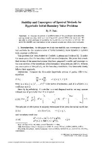
7. SOME NUMERICAL CONSIDERATION The practical implementation of the recursion (15) requires the evaluation of a certain number of the Laurent coe�cients {�j }j¿0 of the mapping relative to a compact subset � containing �(A). In general, �(A) is not known and it is necessary to estimate it using some eigenvalue method (see e.g. References [7, 8, 20, 21]). Consequently, � is usually de�ned as the convex polygonal compact obtained joining the outermost points of the estimate set [20]. For the evaluation of the Laurent coe�cients {�j }j¿0 of , in our tests we employed the software SC Matlab Toolbox, written by Driscoll in 1995 (see Reference [22]). We must point out that especially when � is convex, a small number of computed leading coe�cients of usually allows to get a good approximation of �. In Figure 1, we can see some examples of convex polygonal domains and the approximations obtained computing l (de�ned at the top of each picture) leading coe�cients of the corresponding . In general, always assuming that � is convex, the choice of l = 10 usually leads to good results. Hence, numerically, the mapping with its (generally in�nite) development is replaced by an approximation ˜ (w) = w + �˜0 + �˜1 + �˜2 + · · · + �˜l ; w w2 wl
|w|¿˜�
with �˜ ≈ �. The implementation of the recursion (15) requires also the evaluation of the Faber coe�cients aj (�), j ¿0. After computing ˜ , the computation of the Faber coe�cients can be performed using any suitable quadrature formula. Anyway one can also use the following result. Proposition 7.1 For j ¿1, aj−1 (�) + Copyright ? 2002 John Wiley & Sons, Ltd.
� j aj (�) = ∞ i=1 i�i aj+i (�) �
(55)
Numer. Linear Algebra Appl. 2003; 10:247–270
263
SOLVING LINEAR INITIAL VALUE PROBLEMS
l=4
l=4
3
3
2
2
1
1
0
0
_ 1
_1
_2
_2
_3 _ 0.5
0
0.5
1
1.5
2
2.5
_3 _ 0.5
0
0.5
l=6 3
2
2
1
1
0
0
_1
_1
_2
_2
0
0.5
1.5
2
2.5
1.5
2
2.5
l=6
3
_3 _ 0.5
1
1
1.5
2
2.5
_3 _ 0.5
0
0.5
1
Figure 1.
Proof Integrating by parts aj (�); j ¿1, and by (10), we get aj (�) =
1 2�i
=−
� |w|=R
� 1 j 2�i
� 1 =− j 2�i
exp(−� (w)) dw; wj+1
�
R¿�
|w|=R
exp(−� (w)) wj
|w|=R
� � exp(−� (w)) �1 2�2 1 − 2 − 3 − · · · dw wj w w
�
�
(w) dw
that proves the thesis. Clearly, on replacing by ˜ , formula (55) has a �nite number l + 2 of terms. It generalizes the well-known recursion for Chebyshev coe�cients that can be expressed in terms of modi�ed Bessel functions (see e.g. Reference [13]). As for Chebyshev coe�cients, formula Copyright ? 2002 John Wiley & Sons, Ltd.
Numer. Linear Algebra Appl. 2003; 10:247–270
264
P. NOVATI
(55) cannot be used forward, in view of its instability. Once a priori estimate of the required number m of coe�cients is available (using for instance a priori upper bound for the error of approximation), after computing am+1 (�); am+2 (�) : : : ; am+j (�), recursion (55) must be used backward. We observe that for both F[m; k] and F[m], the mapping ˜ and the Faber coe�cients have to be computed only once, at the beginning. Together with the above numerical consideration, here we want to show an improvement of the bound (22) for the exponential function, i.e. |aj (�)|6
e−� (−R) Rj
(56)
Proposition 7.2 � For each R¿� we have Let � ∈ M. |a0 (�)| 6 e−�
(−R)
� |aj (�)| 6 j−1 e−� jR
� (−R)
1+
� � 2 �
R
j ¿1
;
(57)
Proof For j = 0 the thesis follows immediately by (13) and the geometry of �. For j ¿1, using integration by parts we get aj (�) =
1 2�i
=−
� |u|=R
� 1 j 2�i
exp(−� (u)) du u j+1
�
|u|=R
exp(−� (u)) uj
�
(u) du
(58)
Now, using the bound (see Reference [11]) | � (Rei )|61 +
� � 2
R
;
R¿�
we get the thesis for j ¿1. � j (�), j ¿0, as the bounds for |aj (�)| given by (56) and (57), reDe�ning �j (�) and � spectively, the following tables show a comparison between these two bounds for � = 0:05 and � = 0:01, in the case of an ellipse. In particular we consider the ellipse associated with the conformal mapping (w) = w + 5 + 2=w, with capacity � = 4. For the bounds we choose R = �. As we can see, the di�erence between the two estimates appears more evident as � becomes smaller. The improvement given by (57) is of particular importance when � → 0, because � j (�) → 0 for j¿0 (see (57)), as the corresponding exact � 0 (�) → 1 and � in this situation � values |aj (�)|. Note that Proposition 7.2 can be used to improve the bounds (21) and (26). However, such an improvement does not allow to attain qualitatively better results in Section 6. Copyright ? 2002 John Wiley & Sons, Ltd.
Numer. Linear Algebra Appl. 2003; 10:247–270
SOLVING LINEAR INITIAL VALUE PROBLEMS
j
|aj (�)|
�j (�)
� j (�) �
0 1 2 3 4 5 0 1 2 3 4 5
7.8E-1 3.9E-2 6.5E-5 1.1E-9 ¡1E-14 ¡1E-14 9.5E-1 9.5E-3 6.3E-7 8E-14 ¡1E-14 ¡1E-14
9.7E-1 2.4E-1 6.1E-2 1.5E-2 3.8E-3 9.5E-4 9.9E-1 2.5E-1 6.2E-2 1.5E-2 3.9E-3 9.7E-4
9.7E-1 9.7E-2 1.2E-2 2.0E-3 3.8E-4 7.6E-5 9.9E-1 2.0E-2 2.5E-3 4.1E-4 7.7E-5 1.5E-5
265
8. NUMERICAL EXPERIMENTS The problems we consider arise from the semi-discretization of the parabolic equation @u(x; y; z; t) @u(x; y; z; t) @u(x; y; z; t) = �u(x; y; z; t) − �1 + r(x; y; z; t) − �2 @t @x @y x; y; z ∈ (0; 1);
� 1 ; �2 ∈ R
u(x; y; z; t) = 0
for (x; y; z) on the boundary
where � is the three-dimensional Laplacian operator, using central di�erences on a uniform meshgrid of n + 2 points in each direction. The semi-discretization yields usual systems of ordinary linear di�erential equations of the type y� (t) = −Ay(t) + g(t);
t ∈ [0; T ]
y(0) = y0
(59)
where A ∈ RN ×N , with N = n3 , and g : [0; T ] → RN . De�ning h = 1=(n + 1), and
� � � � � �21 h2 �22 h2 n := cos + 1− +1 1− n+1 4 4 �(A) is contained in the rectangle (1=h2 )Rn , where Rn := [6 − 2 Re n ; 6 + 2 Re n ] × [−2i Im n ; 2iIm n ]: In order to provide an estimate for F(A) of this example we use the following result [23, p. 79]. Theorem 8.1 Given A ∈ RN ×N , let M := 12 (A + AT ), M˜ := 12 (A − AT ). Then F(A) ⊆ [a; b] × [−ic; ic] Copyright ? 2002 John Wiley & Sons, Ltd.
(60)
Numer. Linear Algebra Appl. 2003; 10:247–270
266
P. NOVATI
where a, b, c, are such that F(M ) = [a; b], F(M˜ ) = [−ic; ic]. The rectangle (60) is the smallest that contains F(A). In our case, M is the matrix obtained discretizing as before the Laplacian operator, so that � � � � 6 ; 1 + cos F(M ) = 2 1 − cos h n+1 n+1 and for M˜ , we have
� � � � 2(�1 + �2 ) ˜ ; i cos −i cos F(M ) = h n+1 n+1
Therefore, once the conformal mapping relative to (1=h2 )Rn has been computed, the smallest value s such that �(s) ⊇ F(A), can be estimated by solving � � � � 2(�1 + �2 ) 6 cos (61) +i (w) = 2 1 − cos h n+1 h n+1 If w˜ is the solution of (61), then s6|w˜ |. In the following numerical examples we make a comparison between the Faber exponential integrators (39) and (41) built on the compact � := (1=h2 )Rn and some Krylov exponential integrators. In particular we consider the standard Arnoldi exponential integrator, extensively studied in References [1, 6], implemented with the modi�ed Gram–Schmidt process without reorthogonalization. We also consider the exponential integrator based on the incomplete Arnoldi process of order P, that we denote with Arnoldi (P). For this method, various numerical experiments on our example reveal that the choice of P = 4 is the most convenient in the sense of the convergence rate with respect to the total amount of work. Finally, we consider the exponential integrator based on the Lanczos biorthogonalization algorithm, studied in References [2, 3]. Since all these approaches are of polynomial type like the FSM, we can make an e�ective comparison simply by choosing, for each problem, corresponding integrators (cf. Section 5 and Reference [1]). We integrate equations of type (59) between 0 and T , varying the time step �. The degree m of the two methods at each step is chosen so that the �nal error, i.e. the error at time T (err in the tables below), is almost equal for all the methods. Our aim is to give particular attention to the computational costs of the methods relative to similar accuracy results. Computational costs are considered in terms of number of scalar products (nsp). In this context, we must point out that an application of A costs about as much as seven scalar products. In order to understand how much work would be required for problems with a less sparse matrix, we remark that the number of matrix–vector products is equal to the degree m for the Faber and the Arnoldi based exponential integrators, whereas it is equal to 2m for the Lanczos-based method. In all tests Faber methods are built computing only the �rst four leading Laurent coe�cients of the mapping relative to (1=h2 )Rn , i.e., we approximate by ˜ (w) = w + �˜0 + �˜1 + �˜2 + �˜3 w w2 w3 so that the corresponding recurrence relation for Faber polynomials involves six terms (cf. Section 3). Copyright ? 2002 John Wiley & Sons, Ltd.
Numer. Linear Algebra Appl. 2003; 10:247–270
267
SOLVING LINEAR INITIAL VALUE PROBLEMS
Table I. Arnoldi �1
Faber
�2
T
�
m
nsp
err
m
nsp
err
50
20
0.05
70
50
0.02
100
100
0.02
0.05 0.025 0.01 0.005 0.02 0.01 0.005 0.002 0.02 0.01 0.005 0.002
50 40 18 12 56 38 26 15 80 48 28 16
1605 2168 1449 1572 1965 1983 2090 2190 3768 2985 2363 2416
2.20E-9 2.99E-9 2.49E-8 4.21E-9 8.51E-9 4.62E-9 5.78E-9 2.69E-9 1.30E-9 1.44E-9 5.91E-9 1.14E-9
70 36 18 11 62 38 25 17 85 47 26 15
455 462 561 660 402 488 633 1056 554 607 660 924
1.57E-9 3.34E-9 1.85E-9 2.84E-9 6.61E-9 6.81E-9 6.42E-9 6.28E-9 1.31E-9 1.05E-9 4.93E-9 1.16E-9
Arnoldi (4) 50
20
0.05
70
50
0.02
100
100
0.02
0.05 0.025 0.01 0.005 0.02 0.01 0.005 0.002 0.02 0.01 0.005 0.002
75 38 20 12 63 38 24 14 83 48 29 16
789 793 1030 1212 661 793 993 1424 873 1005 1205 1663
Lanczos 2.92E-9 4.18E-9 1.44E-9 2.59E-9 6.49E-9 6.94E-9 3.86E-9 2.04E-9 5.41E-9 2.92E-9 4.22E-9 1.44E-9
65 40 25 14 60 37 30 16
988 1216 1900 2128 912 1124 1824 2432
2.36E-9 0.24E-9 6.20E-9 1.67E-8 8.49E-9 2.98E-9 2.38E-9 4.96E-9
32 18
1945 2736
1.75E-8 3.33E-9
Remark 8.1 For our test problem, we use a matrix whose spectrum is explicitly known. Anyway, it is worth noting that we do not use the spectral decomposition of the matrix, but only the convex hull of its spectrum. 8.1. A non-symmetric model problem In the �rst test problem we de�ne n = 15, i.e. N = 3375, h = 1=16, g ≡ 0, y0 = (1; 1; : : : ; 1)T and vary �1 , �2 . Since g ≡ 0, the problem simply consists of computing a certain number of matrix exponentials. Hence we compare the F[m] method with the corresponding Arnoldi, Arnoldi (4) and Lanczos schemes. In Table I we can note that even if, in most of the tests, the number of iterations m of the Krylov methods is less than the corresponding m of the Faber method, in terms of the number of scalar products the F[m] method performs surely better. This di�erence of costs is particularly evident with respect to the Arnoldi method for large (with respect to T ) values of �, because in this situation, to get a certain accuracy, m has to be chosen su�ciently large. In fact, as well known, the cost of each Arnoldi step increases with the number of iterations. Copyright ? 2002 John Wiley & Sons, Ltd.
Numer. Linear Algebra Appl. 2003; 10:247–270
268
P. NOVATI
Table II. Arnoldi
Faber
�1
�2
T
�
m
nsp
err
m
nsp
err
60
0
0.1
40
20
0.1
0.1 0.05 0.02 0.01 0.005 0.1 0.05 0.025 0.01 0.005
50 48 40 30 21 47 46 44 30 20
3210 4478 6504 7293 7761 2876 4153 6402 7293 7182
1.11E-9 3.07E-9 6.31E-9 1.70E-9 2.11E-9 4.84E-9 9.50E-9 1.08E-9 1.60E-9 3.19E-9
66 64 46 34 26 55 53 50 35 25
858 1247 1782 2395 3465 713 1029 1617 2468 3326
1.64E-9 3.48E-9 4.74E-9 2.58E-9 1.12E-9 5.25E-9 6.01E-9 1.49E-9 0.64E-9 4.03E-9
Arnoldi (4) 60
40
0
20
0.1
0.1
0.1 0.05 0.02 0.01 0.005 0.1 0.05 0.025 0.01 0.005
70 68 60 31 22 57 57 48 31 21
1472 2144 3780 3548 4771 1196 1794 2514 3548 4548
1.11E-9 3.07E-9 6.31E-9 1.70E-9 2.11E-9 4.84E-9 9.50E-9 1.08E-9 1.60E-9 3.19E-9
Lanczos 60
1824
2.57E-9
30 21 55
5016 6073 1672
2.43E-8 1.63E-8 8.63E-9
23
7341
5.75E-9
For this reason, especially when m is large, the incomplete version Arnoldi(4) represents an e�ective schemes. Regarding the Lanczos method, the experiments show that sometimes it does not allow to attain the accuracy of the other methods. Moreover, the empty lines in the table below indicates that the Lanczos method is very unstable and does not converge (the same is valid for the Tables II and III). 8.2. A non-symmetric model problem with forcing term As before we de�ne n = 15, i.e. N = 3375, y0 = (1; 1; : : : ; 1)T . In Table II some tests on a problem (59) with time constant forcing term g = y0 , are shown. Regarding the computational cost, all consideration given for the previous example remains valid also for this one. In this example we use iteration (43) for all the methods and, in order to optimize the cost, it is also possible to distinguish between the number of iterations performed to compute the matrix exponential (m1 ) and that for the computation of ’(�A) (m2 ). In any case, the relationship between the costs of the methods is substantially independent of this choice. In Table III we can observe some tests on a problem (59) with the time varying forcing term g(t) = y0 t. Since we use the scheme described by (39) we need a quadrature formula. The formula chosen (q in Table III) is the Simpson rule built on k points that we indicate with Sk . Therefore, the weights (�1 ; �2 ; �3 ; : : : ; �k ) of (39) are given by ( 13 ; 43 ; 23 ; : : : ; 13 ). Copyright ? 2002 John Wiley & Sons, Ltd.
Numer. Linear Algebra Appl. 2003; 10:247–270
269
SOLVING LINEAR INITIAL VALUE PROBLEMS
Table III. Arnoldi
Faber
�1
�2
T
�
q
m
nsp
err
m
nsp
err
40
0
0.1
0.1 0.05 0.025 0.02 0.01
S9 S7 S7 S7 S5
20 25 16 16 20
2736 6370 6523 8214 16758
7.29E-3 3.28E-3 2.14E-3 1.25E-3 1.26E-4
25 30 25 25 25
1267 2488 4276 5385 7761
7.32E-3 3.42E-3 2.66E-3 1.61E-3 1.27E-4
Arnoldi (4) 40
0
0.1
0.1 0.05 0.025 0.02 0.01
S9 S7 S7 S7 S5
26 30 18 17 20
2156 4056 4989 5922 10094
5.97E-3 5.61E-3 7.14E-3 7.07E-3 7.24E-3
Lanczos 20 25 16 16 18
2432 4940 6566 8268 13406
3.81E-3 5.64E-3 7.22E-2 4.13E-2 7.13E-3
As we can see, the behaviour is similar to that of previous examples. It is not much useful to give more complicated tests, because all the methods are applied in the same manner and the only important di�erence is given by the computation of the matrix functions.
9. FINAL REMARKS In our tests we are supposed to know the exact location of the spectrum of the matrix A, that is, the rectangle (1=h2 )Rn . However, as explained in Section 7, when �(A) is not known the implementation of the Faber expansion method requires a preliminary work to locate it. Some authors consider such preliminary phase as a serious drawback of expansion methods for matrix functions. Anyway, for practical problems like (1), where more than one or a lot of matrix functions always with the same matrix must be computed, the cost of the preliminary phase is surely negligible with respect to the total amount of work (see e.g. References [8, 13]). Moreover, other numerical experiments show that when the function involved is analytic in the whole complex plane as in (1), even a poor approximation of �(A) leads to acceptable results. For these reasons, in the author’s opinion, the Faber expansion method actually constitutes an e�cient alternative to the Krylov approaches for (1) based on the Arnoldi or Lanczos algorithms and their variants, especially when the matrix of the problem is large and sparse as in the case considered for the numerical experiments. REFERENCES 1. Gallopoulos E, Saad Y. E�cient solution of parabolic equations by Krylov approximation methods. SIAM Journal on Statistical and Scienti�c Computing 1992; 13:1236 –1264. 2. Hochbruck M, Lubich C. On Krylov subspace approximation to the matrix exponential operator. SIAM Journal on Numerical Analysis 1995; 34(5):1911–1925. 3. Hochbruck M, Lubich C. Exponential integrators for quantum-classical molecular dynamics. BIT 1999; 39: 620 – 645. Copyright ? 2002 John Wiley & Sons, Ltd.
Numer. Linear Algebra Appl. 2003; 10:247–270
270
P. NOVATI
4. Hochbruck M, Lubich C, Selhofer H. Exponential integrators for large systems of di�erential equations. SIAM Journal on Scienti�c Computing 1998; 19:1552–1574. 5. Knizhnerman L. Calculation of functions of unsymmetric matrices using Arnoldi’s method. Computational Mathematics and Mathematical Physics 1991; 31(1):1– 9 (English Edition by Pergamon Press: Oxford). 6. Saad Y. Analysis of some Krylov subspace approximations to the matrix exponential operator. SIAM Journal on Numerical Analysis 1992; 29:209 –228. 7. Moret I, Novati P. The computation of functions of matrices by truncated Faber series. Numerical Functional Analysis and Optimization 2001; 22:697–719. 8. Novati P. Polynomial methods for the computation of functions of large unsymmetric matrices. Ph.D. Thesis, Universit a degli Studi di Padova, 2000. 9. Curtiss JH. Faber polynomials and Faber series. American Mathematical Monthly 1971; 78:577– 596. 10. Ellacott SW. Computation of Faber series with application to numerical polynomial approximation in the complex plane. Mathematics of Computation 1983; 40:575 – 587. 11. Kovari T, Pommerenke C. On Faber polynomials and Faber expansions. Mathematische Zeitschrift 1967; 99:193 –206. 12. Smirnov VI, Lebedev NA. Functions of a complex variable—constructive theory. MIT Press: Cambridge, MA, 1968. 13. Bergamaschi L, Vianello M. E�cient computation of the exponential operator for large, sparse, symmetric matrices. Numerical Linear Algebra with Applications 2000; 7(1):27– 45. 14. Tal-Ezer H. Spectral methods in time for hyperbolic equations. SIAM Journal on Numerical Analysis 1986; 23:11– 26. 15. Tal-Ezer H. Spectral methods in time for parabolic problems. SIAM Journal on Numerical Analysis 1989; 26:1–11. 16. Eiermann M. On semiiterative methods generated by Faber polynomials. Numerische Mathematik 1989; 56:139 –156. 17. Eiermann M, Niethammer W, Varga RS. A study of semiiterative methods for nonsymmetric systems of linear equations. Numerische Mathematik 1985; 47:505 – 533. 18. Eiermann M. Fields of values and iterative methods. Linear Algebra and Its Applications 1993; 180:167–197. 19. Spijker MN. Numerical ranges and stability estimates. Applied Numerical Mathematics 1993; 13:241– 249. 20. Starke G, Varga RS. A hybrid Arnoldi–Faber iterative method for nonsymmetric systems of linear equations. Numerische Mathematik 1993; 64:213 –240. 21. Manteu�el TA, Starke G. On hybrid iterative methods for nonsymmetric systems of linear equations. Numerische Mathematik 1996; 73:489 – 506. 22. Driscoll TA. Algorithm 756: A MATLAB toolbox for Schwarz–Christo�el mapping. ACM Transactions on Mathematical Software 1996; 22(2):168 –186. 23. Householder AS. The Theory of Matrices in Numerical Analysis. Blaisdell: New York, 1964.
Copyright ? 2002 John Wiley & Sons, Ltd.
Numer. Linear Algebra Appl. 2003; 10:247–270