Solving log-determinant optimization problems by a Newton-CG primal proximal point algorithm Chengjing Wang ∗, Defeng Sun † and Kim-Chuan Toh
‡
September 29, 2009 Abstract We propose a Newton-CG primal proximal point algorithm for solving large scale log-determinant optimization problems. Our algorithm employs the essential ideas of the proximal point algorithm, the Newton method and the preconditioned conjugate gradient solver. When applying the Newton method to solve the inner sub-problem, we find that the log-determinant term plays the role of a smoothing term as in the traditional smoothing Newton technique. Focusing on the problem of maximum likelihood sparse estimation of a Gaussian graphical model, we demonstrate that our algorithm performs favorably comparing to the existing stateof-the-art algorithms and is much more preferred when a high quality solution is required for problems with many equality constraints.
Keywords: Log-determinant optimization problem, Sparse inverse covariance selection, Proximal-point algorithm, Newton’s method
1
Introduction
In this paper, we consider the following standard primal and dual log-determinant (logdet) problems: (P )
min{hC, Xi − µ log det X : A(X) = b, X Â 0},
(D)
max {bT y + µ log det Z + nµ(1 − log µ) : Z + AT y = C, Z Â 0},
X
y,Z
∗
Singapore-MIT Alliance, 4 Engineering Drive 3, Singapore 117576 (
[email protected]). Department of Mathematics and NUS Risk Management Institute, National University of Singapore, 2 Science Drive 2, Singapore 117543 (
[email protected]). The research of this author is partially supported by the Academic Research Fund Under Grant R-146-000-104-112. ‡ Department of Mathematics, National University of Singapore, 2 Science Drive 2, Singapore 117543 (
[email protected]); and Singapore-MIT Alliance, 4 Engineering Drive 3, Singapore 117576. †
1
where S n is the linear space of n × n symmetric matrices, C ∈ S n , b ∈ Rm , µ ≥ 0 is a given parameter, and h·, ·i stands for the standard trace inner product in S n . Here A : S n → Rm is a linear map and AT : Rm → S n is the adjoint of A. We assume that A is surjective, and hence AAT is nonsingular. The notation X Â 0 means that X is a n symmetric positive definite matrix. We further let S+n (resp., S++ ) to be the cone of n × n symmetric positive semidefinite (resp., definite) matrices. Note that the linear maps A and AT can be expressed, respectively, as h iT A(X) = hA1 , Xi, . . . , hAm , Xi ,
T
A (y) =
m X
yk A k ,
k=1
where Ak , k = 1, · · · , m are given matrices in S n . It is clear that the log-det problem (P ) is a convex optimization problem, i.e., the n objective function hC, Xi − µ log det X is convex (on S++ ), and the feasible region is convex. The log-det problems (P ) and (D) can be considered as a generalization of linear semidefinite programming (SDP) problems. One can see that in the limiting case where µ = 0, they reduce, respectively, to the standard primal and dual linear SDP problems. Log-det problems arise in many practical applications such as computational geometry, statistics, system identification, experiment design, and information and communication theory. Thus the algorithms we develop here can potentially find wide applications. One may refer to [5, 25, 22] for an extensive account of applications of the log-det problem. For small and medium sized log-det problems, including linear SDP problems, it is widely accepted that interior-point methods (IPMs) with direct solvers are generally very efficient and robust; see for example [22, 23]. For log-det problems with m large and n moderate (say no more than 2, 000), the limitations faced by IPMs with direct solvers become very severe due to the need of computing, storing, and factorizing the m × m Schur matrices that are typically dense. Recently, Zhao, Sun and Toh [29] proposed a Newton-CG augmented Lagrangian (NAL) method for solving linear SDP problems. This method can be very efficient when the problems are primal and dual nondegenerate. The NAL method is essentially a proximal point method applied to the primal problem where the inner sub-problems are solved by an inexact semi-smooth Newton method using a preconditioned conjugate gradient (PCG) solver. Recent studies conducted by Sun, Sun and Zhang [21] and Chan and Sun [6] revealed that under the constraint nondegenerate conditions for (P ) and (D) (i.e., the primal and dual nondegeneracy conditions in the IPMs literature, e.g., [1]), the NAL method can locally be regarded as an approximate generalized Newton method applied to a semismooth equation. The latter result may explain to a large extent why the NAL method can be very efficient. As the log-det problem (P ) is an extension of the primal linear SDP, it is natural for us to further use the NAL method developed for linear SDPs to solve log-det problems. Following what has been done in linear SDPs, our approach is to apply a Newton-CG primal proximal point algorithm (PPA) to (1), and then to use an inexact Newton method 2
to solve the inner sub-problems by using a PCG solver to compute inexact Newton directions. We note that when solving the inner sub-problems in the NAL method for linear SDPs [29], a semi-smooth Newton method has to be used since the objective functions are differentiable but not twice continuously differentiable. But for log-det problems, the objective functions in the inner sub-problems are twice continuously differentiable (actually, analytic) due to the fact that the term −µ log det X acts as a smoothing term. This interesting phenomenon implies that the standard Newton method can be used to solve the inner sub-problem. It also reveals a close connection between adding the log-barrier term −µlog detX to a linear SDP and the technique of smoothing the KKT conditions [6]. In [19, 20], Rockafellar established a general theory on the global convergence and local linear rate of convergence of the sequence generated by the proximal point and augmented Lagrangian methods for solving convex optimization problems including (P ) and (D). Borrowing Rockafellar’s results, we can establish global convergence and local convergence rate for our Newton-CG PPA method for (P ) and (D) without much difficulty. In problem (P ), we only deal with a matrix variable, but the PPA method we develop in this paper can easily be extended to the following more general log-det problems to include vector variables: min{hC, Xi − µ log det X + cT x − ν log x : A(X) + Bx = b, X Â 0, x > 0},
(1)
max{bT y + µ log det Z + ν log z + κ : Z + AT y = C, z + B T y = c, Z Â 0, z > 0},
(2)
where ν > 0 is a given parameter, c ∈ Rl and B ∈ Rm×l are given data, and κ = nµ(1 − log µ) + lν(1 − log ν). In the implementation of our Newton-CG PPA method, we focus on the maximum likelihood sparse estimation of a Gaussian graphical model (GGM). This class of problems includes two subclasses. The first subclass is that the conditional independence of a model is completely known, and it can be formulated as follows: n o (3) min hS, Xi − log detX : Xij = 0, ∀ (i, j) ∈ Ω, X Â 0 , X
where Ω is the set of pairs of nodes (i, j) in a graph that are connected by an edge, and S ∈ S n is a given sample covariance matrix. Problem (3) is also known as a sparse covariance selection problem. In [7], Dahl, Vandenberghe and Roychowdhury showed that when the underlying dependency graph is nearly-chordal, an inexact Newton method combined with an appropriate PCG solver can be quite efficient in solving (3) with n up to 2, 000 but on very sparse data (for instance, when n = 2, 000, the number of upper nonzeros is only about 4, 000 ∼ 6, 000). But for general large scale problems of the form (3), little research has been done in finding efficient algorithms to solve the problems. The second subclass of the GGM is that the conditional independence of the model is partially known, and it is formulated as follows: n o X (4) min hS, Xi − log det X + ρij |Xij | : Xij = 0, ∀ (i, j) ∈ Ω, X Â 0 . X
(i,j)6∈Ω
3
In [8], d’Aspremont, Banerjee, and El Ghaoui, among the earliest, proposed to apply Nesterov’s smooth approximation (NSA) scheme to solve (4) for the case where Ω = ∅. Subsequently, Lu [11, 12] suggested an adaptive Nesterov’s smooth (ANS) method to solve (4). The ANS method is currently one of the most effective methods for solving large scale problems (e.g., n ≥ 1, 000, m ≥ 500, 000) of the form (4). In the ANS method, the equality constraints in (4) are removed and included in the objective function via the penalty approach. The main idea in the ANS method is basically to apply a variant of Nesterov’s smooth method [17] to solve the penalized problem subject to the single constraint X Â 0. In fact, both the ANS and NSA methods have the same principle idea, but the latter runs much slowly than the former. In contrast to IPMs, the greatest merit of the ANS method is that it needs much lower storage and computational cost per iteration. In [11], the ANS method has been demonstrated to be rather efficient in solving randomly generated problems of form (4), while obtaining solutions with low/moderate accuracy. However, as the ANS is a first-order method, it may require huge computing cost to obtain high accuracy solutions. In addition, as the penalty approach is used in the ANS method to solve (4), the number of iterations may increase drastically if the penalty parameter is updated frequently. Another limitation of the ANS method introduced in [11] is that it can only deal with the special equality constraints in (4). It appears to be difficult to extend the ANS method to deal with more general equality constraints of the form A(X) = b. Our numerical results show that for both problems (3) and (4), our Newton-CG PPA method can be very efficient and robust in solving large scale problems generated as in [8] and [11]. Indeed, we are able to solve sparse covariance selection problems with n up to 2, 000 and m up to 1.8 × 10⁶ in about 54 minutes. For problem (4), our method consistently outperforms the ANS method by a substantial margin, especially when the problems are large and the required accuracy tolerances are relatively high. The remaining part of this paper is organized as follows. In Section 2, we give some preliminaries including a brief introduction on concepts related to the proximal point algorithm. In Section 3 and 4, we present the details of the PPA method and NewtonCG algorithm. In Section 5, we give the convergence analysis of our PPA method. The numerical performance of our algorithm is presented in Section 6. Finally, we give some concluding remarks in Section 7.
2
Preliminaries
For the sake of subsequent discussions, we first introduce some concepts related to the proximal point method based on the classic papers by Rockafellar [19, 20]. Let H be a real Hilbert space with an inner product h·, ·i. A multifunction T : H ⇒ H is said to be a monotone operator if hz − z 0 , w − w0 i ≥ 0, whenever w ∈ T (z), w0 ∈ T (z 0 ). 4
(5)
It is said to be maximal monotone if, in addition, the graph G(T ) = {(z, w) ∈ H × H| w ∈ T (z)} is not properly contained in the graph of any other monotone operator T 0 : H ⇒ H. For example, if T is the subdifferential ∂f of a lower semicontinuous convex function f : H → (−∞, +∞], f 6≡ +∞, then T is maximal monotone (see Minty [14] or Moreau [15]), and the relation 0 ∈ T (z) means that f (z) = min f . Rockafellar [19] studied a fundamental algorithm for solving 0 ∈ T (z),
(6)
in the case of an arbitrary maximal monotone operator T . The operator P = (I + λT )−1 is known to be single-valued from all of H into H, where λ > 0 is a given parameter. It is also nonexpansive: kP (z) − P (z 0 )k ≤ kz − z 0 k, and one has P (z) = z if and only if 0 ∈ T (z). The operator P is called the proximal mapping associate with λT , following the terminology of Moreau [15] for the case of T = ∂f . The PPA generates, for any starting point z 0 , a sequence {z k } in H by the approximate rule: z k+1 ≈ (I + λk T )−1 (z k ). Here {λk } is a sequence of positive real numbers. In the case of T = ∂f , this procedure reduces to n o 1 z k+1 ≈ arg min f (z) + kz − zk k2 . (7) z 2λk Definition 2.1. (cf. [19]) For a maximal monotone operator T , we say that its inverse T −1 is Lipschitz continuous at the origin (with modulus a ≥ 0) if there is a unique solution z¯ to z = T −1 (0), and for some τ > 0 we have kz − z¯k ≤ akwk, where z ∈ T −1 (w) and kwk ≤ τ. We state the following lemma which will be needed later in the derivation of the PPA method for solving (P ). Lemma 2.1. Let Y be an n × n symmetric matrix with eigenvalue decomposition Y = P DP T with D = diag(d). We assume that d1 ≥ · · · ≥pdr > 0 ≥ dr+1 · · · ≥ dn . Let x2 + 4γ + x)/2 and φ− γ > 0 be given. For the two scalar functions φ+ γ (x) := γ (x) := ( p 2 ( x + 4γ − x)/2 for all x ∈ 0, where φ+ γ is defined by (8) in Lemma 2.1. Recall that for the linear SDP case (where µ = 0), the complementarity condition XZ = 0 with X, Z º 0, is equivalent to Π+ (X − λZ) = X, for any λ > 0, where Π+ (·) is the metric projector onto S+n . One can see from (12) that when µ > 0, the log-barrier term µlog detX in (P ) contributed to a smoothing term in the projector Π+ . Lemma 3.1. Given any Y ∈ S n and λ > 0, we have n1 o 1 − min kY − Zk2 − µ log det Z = kφ (Y )k2 − µ log det(φ+ γ (Y )), ZÂ0 2λ 2λ γ
(13)
where γ = λµ. Proof. Note that the minimization problem in (13) is an unconstrained problem and the objective function is strictly convex and continuously differentiable. Thus any stationary point would be the unique minimizer of the problem. The stationary point, if it exists, is the solution of the following equation: Y = Z − γZ −1 .
(14)
By Lemma 2.1(a), we see that Z∗ := φ+ γ (Y ) satisfies (14). Thus the optimization problem in (13) has a unique minimizer and the minimum objective function value is given by 1 1 − kY − Z∗ k2 − µ log det Z∗ = kφ (Y )k2 − µ log det(φ+ γ (Y )). 2λ 2λ γ This completes the proof. By defining log 0 := −∞, we can see that problems (P ) and (D) are equivalent to (P 0 )
min{hC, Xi − µ log det X : A(X) = b, X º 0},
(D0 )
max {bT y + µ log det Z : Z + AT y = C, Z º 0}.
X
y,Z
7
Due to this equivalence, from now on we focus on (P 0 ) and (D0 ), rather on (P ) and (D). Let l(X; y) : S n × Rm → R be the ordinary Lagrangian function for (P ) in extended form: ( hC, Xi − µ log det X + hy, b − A(X)i if X ∈ S+n , l(X; y) = (15) ∞ otherwise. The essential objective function in (P 0 ) is given by ( hC, Xi − µ log det X if X ∈ FP , f (X) = maxm l(X; y) = y∈R ∞ otherwise.
(16)
For later developments, we define the following maximal monotone operator associated with l(X, y): Tl (X, y) := {(U, v) ∈ S n × Rm | (U, −v) ∈ ∂l(X, y), (X, y) ∈ S n × Rm }. Let Fλ be the Moreau-Yosida regularization (see [15, 28]) of f in (16) associated with λ > 0, i.e., Fλ (X) = minn {f (Y ) + Y ∈S
1 1 kY − Xk2 } = min {f (Y ) + kY − Xk2 }. n Y ∈S++ 2λ 2λ
(17)
From (16), we have n
o 1 kY − Xk2 Y ∈S++ y∈Rm 2λ n o 1 2 = sup min l(Y ; y) + kY − Xk = sup Θλ (X, y) , n 2λ y∈Rm Y ∈S++ y∈Rm
Fλ (X) =
min sup n
l(Y ; y) +
(18)
where
n o 1 l(Y ; y) + kY − Xk2 Y ∈S++ 2λ o n 1 T 2 = bT y + min hC − A y, Y i − µlog detY + kY − Xk n Y ∈S++ 2λ n1 o 1 1 2 kY − W (X, y)k − µlog detY . = bT y − kWλ (X, y)k2 + kXk2 + min λ n Y ∈S++ 2λ 2λ 2λ
Θλ (X, y) = min n
Here Wλ (X, y) := X − λ(C − AT y). Note that the interchange of min and sup in (18) follows from [18, Corollary 37.3.2]. By Lemma 3.1, the minimum objective value in the above minimization problem is attained at Y∗ = φ+ γ (Wλ (X, y)). Thus we have 1 1 (Wλ (X, y))k2 − µlog det φ+ kXk2 − kφ+ γ (Wλ (X, y)) + nµ. (19) 2λ 2λ γ Note that for a given X, the function Θ(X, ·) is analytic, cf. [24]. Its first and second order derivatives can be computed as in the following lemma. Θλ (X, y) = bT y +
8
Lemma 3.2. For any y ∈ Rm and X Â 0, we have ∇y Θλ (X, y) = b − Aφ+ γ (Wλ (X, y)) 0 T ∇2yy Θλ (X, y) = −λA(φ+ γ ) (Wλ (X, y))A
(20) (21)
Proof. To simplify notation, we use W to denote Wλ (X, y) in this proof. To prove (20), note that 0 + + 0 + −1 ∇y Θ(X, y) = b − A(φ+ γ ) (W )[φγ (W )] − λµA(φγ ) (W )[(φγ (W )) ] 0 + − = b − A(φ+ γ ) (W )[φγ (W ) + φγ (W )].
By Lemma 2.1(c), the required result follows. From (20), the result in (21) follows readily. Let yλ (X) be such that yλ (X) ∈ arg sup Θλ (X, y). y∈Rm
Then we know that φ+ γ (W (X, yλ (X))) is the unique optimal solution to (17). Consequently, we have that Fλ (X) = Θλ (X, yλ (X)) and ∇Fλ (X) =
´ 1 1³ X − φ+ (W (X, y (X))) = C − A T y − φ− (W (X, yλ (X))). λ γ λ λ γ
(22)
n Given X 0 ∈ S++ , the exact PPA for solving (P 0 ), and thus (P ), is given by
X
k+1
−1
n
k
= (I + λk Tf ) (X ) = arg minn
X∈S++
o 1 k 2 kX − X k , f (X) + 2λk
(23)
where Tf = ∂f . It can be shown that k k X k+1 = X k − λk ∇Fλk (X k ) = φ+ γk (W (X , yλk (X ))),
(24)
where γk = λk µ. The exact PPA outlined in (23) is impractical for computational purpose. Hence we consider an inexact PPA for solving (P 0 ), which has the following template.
9
n Algorithm 1: The Primal PPA. Given a tolerance ε > 0. Input X 0 ∈ S++ and λ0 > 0. Set k := 0. Iterate:
Step 1. Find an approximate maximizer y k+1 ≈ arg sup
n
y∈Rm
o θk (y) := Θλk (X k , y) ,
(25)
where Θλk (X k , y) is defined as in (19). Step 2. Compute k k+1 X k+1 = φ+ )), γk (Wλk (X , y
Z k+1 =
1 − φ (Wλk (X k , y k+1 )). λk γk
(26)
Step 3. If kRdk+1 := (X k − X k+1 )/λk k ≤ ²; stop; else; update λk ; end. k k+1 Remark 3.1. Note that b−A(X k+1 ) = b−Aφ+ )) = ∇y Θλk (X k , y k+1 ) ≈ 0. γk (Wλk (X , y
Remark 3.2. Observe that the function Θλ (X, y) is twice continuously differentiable (actually, analytic) in y. In contrast, its counterpart Lσ (y, X) for a linear SDP in [29] fails to be twice continuously differentiable in y and only the Clarke’s generalized Jacobian of ∇y Lσ (y, X) (i.e., ∂∇y Lσ (y, X)) can be obtained. This difference can be attributed to the term −µ log det X in problem (P 0 ). In other words, −µ log det X works as a smoothing term that turns Lσ (y, X) (which is not twice continuously differentiable) into an analytic function in y. This idea is different from the traditional smoothing technique of using a smoothing function on the KKT conditions since the latter is not motivated by adding a smoothing term to an objective function. Our derivation of Θλ (y, X) p shows that the + smoothing technique of using a squared smoothing function φγ (x) = ( x2 + 4γ + x)/2 can indeed be derived by adding the log-barrier term to the objective function. The advantage of viewing the smoothing technique from the perspective of adding a log-barrier term is that the error between the minimum objective function values of the perturbed problem and the original problem can be estimated. In the traditional smoothing technique for the KKT conditions, there is no obvious mean to estimate the error in the objective function value of the solution computed from the smoothed KKT conditions from the true minimum objective function value. We believe the connection we discovered here could be useful for the error analysis of the smoothing technique applied to the KKT conditions. For the sake of subsequent convergence analysis, we present the following proposition. n be the unique optimal Proposition 3.1. Suppose that (P 0 ) satisfies (9). Let X ∈ S++ −1 −1 0 solution to (P ), i.e., X = Tf (0). Then Tf is Lipschitz continuous at the origin.
10
Proof. From [20, Prop. 3], it suffices to show that the following quadratic growth condi¯ for some positive constant α: tion holds at X f (X) ≥ f (X) + αkX − Xk2
∀ X ∈ N such that X ∈ FP
(27)
n where N is a neighborhood of X in S++ . From [4, Theorem 3.137], to prove (27), it suffices to show the second order sufficient condition for (P 0 ) holds. n , we have Now for X ∈ S++ 2 n h∆X, ∇2XX l(X; y)(∆X)i = µhX −1 ∆XX −1 , ∆Xi ≥ µλ−2 max (X)k∆Xk , ∀ ∆X ∈ S ,
where λmax (X) is the maximal eigenvalue of X, this is equivalent to h∆X, ∇2XX l(X; y)(∆X)i > 0, ∀ ∆X ∈ S n \ {0}.
(28)
Certainly, (28) implies the second order sufficient condition for Problem (P 0 ). We can also prove in parallel that the maximal monotone operator Tl is Lipschitz continuous at the origin.
4
The Newton-CG Method for Inner Problems
In the algorithm framework proposed in Section 3, we have to compute y k+1 ≈ argmax {θk (y) : y ∈ Rm }. In this paper, we will introduce the Newton-CG method to achieve this goal.
11
Algorithm 2: The Newton-CG Method. Step 0. Given µ ∈ (0, 12 ), η¯ ∈ (0, 1), τ ∈ (0, 1], τ1 , τ2 ∈ (0, 1), and δ ∈ (0, 1), choose y 0 ∈ Rm . Step 1. For k = 0, 1, 2, . . . , Step 1.1. Given a maximum number of CG iterations nj > 0 and compute. ηj := min{¯ η , k∇y θk (y j )k1+τ }. Apply the CG method to find an approximate solution dj to (∇2yy θk (y j ) + ²j I)d = −∇y θk (y j ),
(29)
where ²j := τ1 min{τ2 , k∇y θk (y j )k}. Step 1.2. Set αj = δ mj , where mj is the first nonnegative integer m for which θk (y j + δ m dj ) ≥ θk (y j ) + µδ m h∇y θk (y j ), dj i. Step 1.3. Set y j+1 = y j + αj dj .
From (21) and the positive definiteness property of φ0+ (W (y; X)) (for some properties of the projection operator one may refer to [13]), we have that −∇2yy θk (y j ) is always positive definite, then −∇2yy θk (y j ) + ²j I is positive definite as long as ∇y θk (y j ) 6= 0. So we can always apply the PCG method to (29). Of course, the direction dj generated from (29) is always an ascent direction. With respect to the analysis of the global convergence and local quadratic convergence rate of the above algorithm, we will not present the details, and one may refer to Section 3.3 of [29] since it is very similar to the semismooth Newton-CG algorithm used in that paper. The difference lies in that dj obtained from (29) in this paper is an approximate Newton direction; in contrast, dj obtained from (62) in [29] is an approximate semimsooth Newton direction.
5
Convergence Analysis
Global convergence and the local convergence rate of our Newton-CG PPA method to problems (P 0 ) and (D0 ) can directly be derived from Rockafellar [19, 20] without much difficulty. For the sake of completeness, we shall only state the results below. Since we cannot solve the inner problems exactly, we will use the following stopping
12
criteria considered by Rockafellar [19, 20] for terminating Algorithm 2: (A) sup θk (y) − θk (y
k+1
)≤
²2k /2λk ,
²k ≥ 0,
∞ X
²k < ∞;
k=0
(B) sup θk (y) − θk (y
k+1
)≤
δk2 /2λk kX k+1
k 2
− X k , δk ≥ 0,
∞ X
δk < ∞;
k=0
(B 0 ) k∇y θk (y k+1 )k ≤ δk0 /λk kX k+1 − X k k, 0 ≤ δk0 → 0. In view of Proposition 3.1, we can directly obtain from [19, 20] the following convergence results. Theorem 5.1. Let Algorithm 1 be executed with stopping criterion (A). If (D0 ) satisfies n condition (10), then the generated sequence {X k } ⊂ S++ is bounded and {X k } converges to X, where X is the unique optimal solution to (P 0 ), and {y k } is asymptotically maximizing for (D0 ) with min(P 0 )=sup(D0 ). If {X k } is bounded and (P 0 ) satisfies condition (9), then the sequence {y k } is also bounded, and the accumulation point of the sequence {y k } is the unique optimal solution to (D0 ). Theorem 5.2. Let Algorithm 1 be executed with stopping criteria (A) and (B). Assume that (D0 ) satisfies condition (10) and (P 0 ) satisfies condition (9). Then the generated n sequence {X k } ⊂ S++ is bounded and {X k } converges to the unique solution X to (P 0 ) 0 0 with min(P )=sup(D ), and kX k+1 − Xk ≤ θk kX k − Xk, for all k sufficiently large, where 2 −1/2 θk = [af (a2f + σk2 )−1/2 + δk ](1 − δk )−1 → θ∞ = af (a2f + σ∞ ) < 1, σk → σ∞ ,
and af is a Lipschitz constant of Tf−1 at the origin. The conclusions of Theorem 5.1 about {y k } are valid. Moreover, if the stopping criterion (B 0 ) is also used, then in addition to the above conclusions the sequence {y k } → y, where y is the unique optimal solution to (D0 ), and one has ky k+1 − yk ≤ θk0 kX k+1 − X k k, for all k sufficiently large, where θk0 = al (1 + δk0 )/σk → δ∞ = al /σ∞ , and al is a Lipschitz constant of Tl−1 at the origin.
13
Remark 5.1. In Algorithm 1 we can also add the term − 2λ1k ky − y k k2 to θk (y). Actually, in our MATLAB code, one can optionally add this term. This actually corresponds to the PPA of multipliers considered in [20, Section 5]. Convergence analysis for this improvement can be conducted in a parallel way as for Algorithm 1. Note that in the stopping criteria (A) and (B), sup θk (y) is an unknown value. Since θk (y) − 2λ1k ky − y k k2 is a strongly concave function with modulus λ1k , then one has the estimate 1 k∇y θk (y k+1 )k2 , sup θk (y) − θk (y k+1 ) ≤ 2λk thus criteria (A) and (B) can be practically modified as follows: k∇y θk (y k+1 )k ≤ ²k , ²k ≥ 0, k∇y θk (y k+1 )k ≤ δk kX k+1 − X k k, δk ≥ 0,
∞ X k=0 ∞ X
²k < ∞; δk < ∞.
k=0
6
Numerical Experiments
In this section, we present some numerical results to demonstrate the performance of our PPA on (3) and (4), for Gaussian graphical models with both synthetic and real data. We implemented the PPA in Matlab. All runs are performed on an Intel Xeon 3.20GHz PC with 4GB memory, running Linux and Matlab (Version 7.6). We measure the infeasibilities and optimality for the primal and dual problems (P ) and (D) as follows: RD =
kC − AT y − Zk , 1 + kCk
RP =
kb − A(X)k , 1 + kbk
RG =
|pobj − dobj| , 1 + |pobj| + |dobj|
(30)
where pobj = hC, Xi − µlog det(X) and dobj = bT y + µlog det(Z) + nµ(1 − log µ). The above measures are similar to those adopted in [29]. In our numerical experiments, we stop the PPA when max{RD , RP } ≤ Tol, (31) where Tol is a pre-specified accuracy tolerance. Note that the third equation XZ = µI in (11) holds up to machine precision because of the way we define Z in (26) in the PPA. Unless otherwise specified, we set Tol = 10−6 as the default. We choose the initial iterate X 0 = I, and λ0 = 1. To achieve faster convergence rate when applying the CG method to solve (29), one may apply a preconditioner to the linear system. But a suitable balance between having an effective preconditioner and additional computational cost must be determined. In our implementation, we simply adopt the preconditioner used in [29], i.e., we use diag(M ) as 14
the preconditioner, where M := −λAAT + ²I, and A is the matrix representation of A with respect to the standard bases of S n×n and Rm , and ² is set to 10−4 . We should note that in the PPA, computing the full eigenvalue decomposition of the matrix Wλk (X k , y) to evaluate the function Θλk (X k , y) in (25) may constitute a major part of the overall computation. Thus it is essential for us to use an eigenvalue decomposition routine that is as efficient as possible. In our implementation, we use the LAPACK routine dsyevd.f (based on a divide-and-conquer strategy) to compute the full eigenvalue decomposition of a symmetric matrix. On our machine, it is about 7 to 10 times faster than Matlab’s eig routine when n is larger than 500. In the ANS method of [12, 11], having an efficient eigenvalue decomposition routine is even more crucial. Thus in our experiments, we also use the faster eigenvalue routine for the ANS method. We focus our numerical experiments on the problems (3) and (4). The problem (4) is not expressed in the standard form given in (1), but it can easily be expressed as such by introducing additional constraints and variables. To be precise, the standard form reformulation of (4) is given as follows: min hC, Xi − µ log det(X) + ρT x+ + ρT x− − ν log x+ − ν log x− s.t. Xij = 0 ∀ (i, j) ∈ Ω − Xij − x+ ij + xij = 0 ∀ (i, j) 6∈ Ω
X Â 0,
(32)
x+ , x− > 0,
where we set ν = 10−16 . We should emphasize that our algorithm is sensitive to the scaling of the data, especially for problem (4). Thus in our implementation, we first scale the data by setting Ak ← Ak /kAk k, C ← C/kCk and b ← b/kbk. In this paper, we mainly compare the performance of our PPA with the ANS method in [11, 12], whose Matlab codes are available at http://www.math.sfu.ca/~zhaosong/. The reason for comparing only with the ANS method is because it is currently the most advanced first order method developed for solving the covariance selection problems (3) and (4). In the ANS method, the convergence criterion is controlled by two parameters ²o , ²c , which stand for the errors in the objective value and primal infeasibility, respectively. b of the As mentioned in [26, 27], we may evaluate the performance of an estimator Σ true covariance matrix Σ by a normalized L2 -loss function which is defined as follows: b − IkF /n. Lloss = kΣ−1 Σ 2 Thus in our numerical experiments, we also report the above value when it is possible to do so.
6.1
Synthetic experiments I
All instances used in this section were randomly generated in a similar manner as described in d’Aspremont et al. [8]. Indeed, we generate a random sparse positive definite matrix 15
n Σ−1 ∈ S++ with a density of about 10% non-zero entries as follows. First we generate an n × n random sparse matrix U with non-zero entries set to ±1. Then set
A = U0 ∗ U; d = diag(A); A = max(min(A − diag(d), 1), −1); B = A + diag(1 + d); Σ−1 = B + max(−1.2 ∗ min(eig(B)), 0.001) ∗ I; The sample covariance matrix S for (3) is generated in a similar manner as in [8], [11] via the following script: E = 2 ∗ rand(n) − 1;
E = 0.5 ∗ (E + E0 );
E = E/kEkF ;
S = Σ + 0.15 ∗ kSigmakF ∗ E; S = S + max(−min(eig(S)), 0.001) ∗ I; The set Ω is generated as in the Matlab codes developed by Lu for the paper [11], specifically, Ω = {(i, j) : (Σ−1 )ij = 0, |i − j| ≥ 5}. In this synthetic experiment, we apply the PPA to the problem (3). The performance of the PPA is presented in Table 1. For each instance in the table, we report the matrix dimension (n); the number of linear constraints (m); the number of outer iterations (it), the total number of sub-problems (itsub) solved by the PPA, and the average number of PCG steps (pcg) taken to solve each linear system; the primal (pobj) and dual (dobj) objective values; the primal (RP ) and dual (RD ) infeasibilities, the relative gap (RG ), and Lloss 2 ; the time (in seconds) taken. We may observe from the table that the PPA can very efficiently solve the problem (3) with synthetic data. Notice that for each of the test b of (3) is not problems, the Lloss value is relatively large, which implies that the solution Σ 2 a good estimate of the true covariance matrix Σ. Table 1: Performance of the PPA on (3) with synthetic data (I). problem
m|n
it/itsub/pcg
rand-500 rand-1000 rand-1500 rand-2000
112405 | 500 450998 | 1000 1015845 | 1500 1806990 | 2000
20| 64| 12.0 20| 58| 9.6 20| 56| 9.9 21| 56| 9.5
pobj 1.03683335 2.40071007 3.88454593 5.45208775
16
RP /RD /RG /Lloss 2
dobj 3 3 3 3
1.03692247 2.40077132 3.88461977 5.45213093
3 3 3 3
1.5-8| 5.2-8| 3.6-8| 1.2-8|
9.1-7| 6.2-7| 7.3-7| 4.3-7|
4.3-5| 1.3-5| 9.5-6| 4.0-6|
2.1 2.9 3.5 4.0
time 0 0 0 0
109.9 510.0 1512.5 3214.5
In Table 2, we compare the performance of our PPA and the ANS method on the first three instances reported in Table 1. For the PPA, Tol in (31) is set to 10−6 , 10−7 and 10−8 ; for ANS, ²o is set to 10−1 , 10−2 and 10−3 , and ²c is set to 10−4 , so that the gap (= |pobj − dobj|) can fall below 10−1 , 10−2 and 10−3 , respectively. For each instance in the table, we give the matrix dimension (n) and the number of linear constraints (m); the gaps achieved, and the times taken (in seconds). From Table 2, we can see that both methods are able to solve all instances within a reasonable amount of time. However, the PPA consistently outperforms the ANS method by about a factor of two when the required accuracy in the computed solution is high. Table 2: Comparison of the PPA and the ANS method on (3) with synthetic data (I). problem
6.2
m|n
rand-500
112405 | 500
rand-1000
450998 | 1000
rand-1500
1015845 | 1500
tolerance PPA (Tol) ANS (²o , ²c ) 10−6 10−7 10−8 10−6 10−7 10−8 10−6 10−7 10−8
(10−1 , 10−4 ) (10−2 , 10−4 ) (10−3 , 10−4 ) (10−1 , 10−4 ) (10−2 , 10−4 ) (10−3 , 10−4 ) (10−1 , 10−4 ) (10−2 , 10−4 ) (10−3 , 10−4 )
gap
time ANS
PPA
ANS
PPA
8.91-2 3.42-3 3.98-4 6.12-2 4.51-3 8.03-4 7.38-2 5.06-3 8.59-4
9.60-2 9.58-3 9.72-4 9.24-2 9.87-3 9.93-4 9.56-2 9.86-3 9.94-4
109.9 140.6 156.4 510.0 604.1 667.3 1512.5 1833.8 2029.1
90.1 159.1 362.4 380.4 696.8 1346.6 1232.1 2308.2 4510.8
Synthetic experiments II
We note that the procedure used in [8] to generate the data matrix S is not in line with the standard practice in statistics. But since the covariance selection problem is a problem in statistics, we prefer to generate the data matrix S according to the standard practice; see for example, [26, 27]. Thus in this sub-section, the true covariance matrices Σ and the index sets Ω are generated exactly the same way as in the previous sub-section. But the sample covariance matrices S are generated differently. For each test problem, we sample 2n instances from the multivariate Gaussian distribution N (0, Σ) to generate a sample covariance matrix S. In the first synthetic experiment, we apply the PPA to the problem (3). The performance of the PPA is presented in Table 3. Again, the PPA can very efficiently solve the problem (3) with S generated from 2n samples of the Guassian distribution N (0, Σ).
17
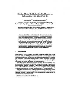
Comparing with Table 1, it appears that the log-det problems in Table 3 are harder to solve when n is large. However, the Lloss value for each problem in the latter table is much 2 smaller than that in the former table. Thus it appears that generating S from sampling the Guassian distribution N (0, Σ) is statistically more meaningful than the procedure used in the previous sub-section. In Figure 1, we show that the PPA can also obtain very accurate solution for the instance rand-500 reported in Table 3 without incurring substantial amount of additional computing time. As can be seen from the figure, the time taken only grows almost linearly when the required accuracy is geometrically reduced. Table 3: Performance of the PPA on (3) with synthetic data (II). problem
m|n
it/itsub/pcg
rand-500 rand-1000 rand-1500 rand-2000
112172 | 500 441294 | 1000 979620 | 1500 1719589 | 2000
19| 20| 23| 22|
42| 46| 56| 52|
16.9 24.0 21.7 20.9
pobj
RP /RD /RG /Lloss 2
dobj
-3.13591727 -9.74364421 -1.91034252 -3.00395927
2 2 3 3
-3.13589617 -9.74359627 -1.91033197 -3.00395142
2 2 3 3
4.2-7| 8.6-7| 7.5-7| 9.8-7|
9.5-7| 3.9-7| 4.7-7| 3.3-7|
3.4-6| 2.5-6| 2.8-6| 1.3-6|
1.7-2 2.0-2 1.8-2 1.5-2
130 120
time (seconds)
110 100 90 80 70 60 50 −4 10
−5
10
−6
−7
10
10
−8
10
−9
10
accuracy
Figure 1: Accuracy versus time for the random instance rand-500 reported in Table 3. In Table 4, we compare the performance of our PPA and the ANS method on the first three instances reported in Table 3. For the PPA, Tol in (31) is set to 3 × 10⁻⁶ , 3 × 10⁻⁷ and 3 × 10⁻⁸ ; for ANS, ²o is set to 10−1 , 10−2 and 10−3 , and ²c is set to 10−4 , so that the gap (= |pobj − dobj|) can fall below 10−1 , 10−2 and 10−3 , respectively. From Table 4, we can see that the PPA consistently outperforms the ANS method by a substantial margin, which ranges from a factor of 5 to 26.
18
time 82.6 765.4 2654.8 5353.4
Table 4: Comparison of the PPA and the ANS method on (3) with synthetic data (II). problem
m|n
tolerance PPA (Tol) ANS (²o , ²c )
rand-500
112172 | 500
rand-1000
441294 | 1000
rand-1500
979620 | 1500
3 × 10⁻⁶ 3 × 10⁻⁷ 3 × 10⁻⁸ 3 × 10⁻⁶ 3 × 10⁻⁷ 3 × 10⁻⁸ 3 × 10⁻⁶ 3 × 10⁻⁷ 3 × 10⁻⁸
(10−1 , 10−4 ) (10−2 , 10−4 ) (10−3 , 10−4 ) (10−1 , 10−4 ) (10−2 , 10−4 ) (10−3 , 10−4 ) (10−1 , 10−4 ) (10−2 , 10−4 ) (10−3 , 10−4 )
gap PPA
ANS
5.58-3 3.05-4 4.45-5 1.35-2 6.04-4 7.64-5 2.23-2 2.36-3 2.51-4
9.79-2 9.94-3 9.94-4 9.91-2 9.94-3 9.94-4 9.94-2 9.94-3 9.94-4
time PPA ANS 75.7 96.3 109.9 704.9 885.3 1006.6 2499.4 2964.2 3429.2
518.3 1233.2 2712.3 4499.8 11715.4 26173.1 13601.7 32440.2 65773.7
In the second synthetic experiment, we consider the problem (4). We set ρij = 1/n1.5 for all (i, j) 6∈ Ω. We note that the parameters ρij are chosen empirically so as to give a b F. reasonably good value for kΣ − Σk In Tables 5 and 6, we report the results in a similar format as those appeared in Table 3 and 4, respectively. Again, we may observe from the tables that the PPA outperformed the ANS method by a substantial margin. Table 5: Performance of the PPA on (4) with synthetic data (II). problem
m|n
it/itsub/pcg
rand-500 rand-1000 rand-1500 rand-2000
112172 | 500 441294 | 1000 979620 | 1500 1719589 | 2000
25| 78| 28| 100| 28| 89| 30| 94|
18.2 30.6 28.9 26.5
pobj -3.11255742 -9.70441465 -1.90500086 -2.99725089
dobj 2 2 3 3
RP /RD /RG
-3.11253082 -9.70433319 -1.90497111 -2.99723060
2 2 3 3
6.5-8| 8.9-9| 5.5-8| 2.1-8|
8.5-7| 4.7-7| 9.4-7| 6.1-7|
4.3-6| 4.2-6| 7.8-6| 3.4-6|
Table 6: Comparison of the PPA and the ANS method on (4) with synthetic data (II). problem
rand-500
m|n
112172 | 500
tolerance PPA (Tol) ANS (²o , ²c ) 3 × 10⁻⁶
(10−1 , 10−4 )
19
gap
time ANS
PPA
ANS
PPA
6.20-3
9.90-2
163.0
510.3
time 1.7-2 2.0-2 1.8-2 1.5-2
173.9 2132.2 5724.1 12217.7
Table 6: Comparison of the PPA and the ANS method on (4) with synthetic data (II). problem
m|n
rand-1000
441294 | 1000
rand-1500
979620 | 1500
6.3
tolerance PPA (Tol) ANS (²o , ²c ) 3 × 10⁻⁷ (10−2 , 10−4 ) 3 × 10⁻⁸ (10−3 , 10−4 ) 3 × 10⁻⁶ (10−1 , 10−4 ) 3 × 10⁻⁷ (10−2 , 10−4 ) 3 × 10⁻⁸ (10−3 , 10−4 ) 3 × 10⁻⁶ (10−1 , 10−4 ) 3 × 10⁻⁷ (10−2 , 10−4 ) 3 × 10⁻⁸ (10−3 , 10−4 )
gap PPA 4.94-4 9.24-5 4.45-2 3.49-3 2.75-4 8.86-2 3.36-3 3.80-4
ANS 9.94-3 9.94-4 9.88-2 9.94-3 9.94-4 9.90-2 9.94-3 9.94-4
time PPA ANS 196.1 1236.9 218.1 2747.0 1839.7 4460.8 2278.7 11562.8 2716.8 26278.6 5254.1 13830.3 6663.0 34208.0 7605.1 73997.1
Real data experiment
In this part, we compare the PPA and the ANS method on two gene expression data sets. Since [2] had already considered these data sets, we can refer to [2] for the choice of the parameters ρij . 6.3.1
Rosetta Inpharmatics Compendium
We applied our PPA and the ANS method to the Rosetta Inpharmatics Compendium of gene expression profiles described by Hughes et al. [9]. The data set contains 253 samples with n = 6136 variables. We aim to estimate the sparse covariance matrix of a Gaussian graphical model whose conditional independence is unknown. Naturally, we formulate it as the problem (4), with Ω = ∅. As for the parameters, we set ρij = 0.0313 as in [2]. As our PPA can only handle problems with matrix dimensions up to about 3000, we only test on a subset of the data. We create 3 subsets by taking 500, 1000, and 2000 variables with the highest variances, respectively. Note that as the variances vary widely, we normalized the sample covariance matrices to have unit variances on the diagonal. In the experiments, we set Tol = 10−6 for the PPA, and (²o , ²c ) = (10−2 , 10−6 ) for the ANS method. The performances of the PPA and ANS methods for the Rosetta Inpharmatics Compendium of gene expression profiles are presented in Table 7. From Table 7, we can see that although both methods can solve the problem, the PPA is nearly two times faster than the ANS method when n = 1500.
20
Table 7: Comparison of the PPA and ANS method on (4) with Ω = ∅ for the Rosetta Inpharmatics Compendiuma data. problem
m|n
Rosetta Rosetta Rosetta
| 500 | 1000 | 1500
6.3.2
tolerance PPA (Tol) ANS (²o ) 10−6 10−6 10−6
10−3 10−3 10−3
primal objective value PPA ANS -7.42643038 2 -1.66546574 3 -2.64937821 3
-7.42642052 2 -1.66546478 3 -2.64937721 3
time PPA ANS 112.7 679.7 1879.8
127.6 881.6 3424.7
Iconix Microarray data
Next we analyze the performances of the PPA and ANS methods on a subset of a 10000 gene microarray data set obtained from 160 drug treated rat livers; see Natsoulis et al. [16] for details. In our first test problem, we take 200 variables with the highest variances from the large set to form the sample covariance matrix S. The other two test problems are created by considering 500 and 1000 variables with the highest variances in the large data set. As in the last data set, we normalized the sample covariance matrices to have unit variances on the diagonal. As the conditional independence of the Gaussian graphical model is not known, we set Ω = ∅ in the problem (4). We set ρij = 0.0853 as in [2]. The performance of the PPA and ANS methods for the Iconix microarray data is presented in Table 8. From the table, we see that the PPA is about two times faster than the ANS method when n = 1000. Table 8: Comparison of the PPA and ANS method on (4) with Ω = ∅ for the Iconix microarray data.
7
problem
m|n
Iconix Iconix Iconix
| 200 | 500 | 1000
tolerance PPA (Tol) ANS (²o ) 10−6 10−6 10−6
10−3 10−3 10−3
primal objective value PPA ANS -6.13127764 0 5.31683807 1 1.78893456 2
-6.13036186 0 5.31688551 1 1.78892330 2
time PPA ANS 51.5 571.6 3510.8
50.7 795.2 7847.3
Concluding Remarks
We designed a primal PPA to solve log-det optimization problems. Rigorous convergence results for the PPA are obtained from the classical results for a generic proximal 21
point algorithm. Extensive numerical experiments conducted on log-det problems arising from sparse estimation of inverse covariance matrices in Gaussian graphical models using synthetic data and real data demonstrated that our PPA is very efficient. In contrast to the case for the linear SDPs, the log-det term used in this paper plays a key role of a smoothing term such that the standard smooth Newton method can be used to solve the inner problem. The key discovery of this paper is the connection of the log-det smoothing term with the technique of using the squared smoothing function. It opens up a new door to deal with nonsmooth equations and understand the smoothing technique more deeply.
Acknowledgements We thank Onureena Banerjee for providing us with part of the test data and helpful suggestions and Zhaosong Lu for sharing with us his Matlab code and fruitful discussions.
References [1] F. Alizadeh, J. P. A. Haeberly, and O. L. Overton, Complementarity and nondegeneracy in semidefinite programming, Mathemtical Programming, 77 (1997), 111–128. [2] O. Banerjee, L. El Ghaoui, A. d’Aspremont, Model selection through sparse maximum likelihood estimation, Journal of Machine Learning Research, 9 (2008), 485–516. [3] R. Bhatia, Matrix Analysis, Springer-Verlag, New York, 1997. [4] J. F. Bonnans and A. Shapiro, Perturbation Analysis of Optimization Problems, Springer, New York, 2000. [5] S. Boyd, L. El Ghaoui, E. Feron, and V. Balakrishnan, Linear matrix inequalities in system and control theory, vol. 15 of Studies in Applied Mathematics, SIAM, Philadelphia, PA, 1994. [6] Z. X. Chan and D. F. Sun, Constraint nondegeneracy, strong regularity and nonsigularity in semidenite programming, SIAM Journal on optimization, 19 (2008), 370–396. [7] J. Dahl, L. Vandenberghe, and V. Roychowdhury, Covariance selection for nonchordal graphs via chordal embedding, Optim. Methods Softw., 23 (2008), 501–520. [8] A. d’Aspremont, O. Banerjee, and L. El Ghaoui, First-order methods for sparse covariance selection, SIAM J. Matrix Anal. Appl., 30 (2008), 56–66.
22
[9] T. R. Hughes, M. J. Marton, A. R. Jones, C. J. Roberts, R. Stoughton, C. D. Armour, H. A. Bennett, E. Coffey, H. Dai, Y. D. He, M. J. Kidd, A. M. King, M. R. Meyer, D. Slade, P. Y. Lum, S. B. Stepaniants, D. D. Shoemaker, D. Gachotte, K. Chakraburtty, J. Simon, M. Bard, and S. H. Friend, Functional discovery via a compendium of expression profiles, Cell, 102(1) 2000, 109C-126. [10] O. Ledoit, and M. Wolf, A well-conditioned estimator for large dimensional covariance matrices, J. of Multivariate Analysis, 88 (2004), pp. 365-411 [11] Z. Lu, Smooth optimization approach for sparse covariance selection, SIAM Journal on Optimization, 19(4) (2009), 1807–1827. [12] Z. Lu, Adaptive first-order methods for general sparse inverse covariance selection, Manuscript, Department of Mathematics, Simon Fraser University, Canada, December 2008. [13] F. Meng, D. F. Sun, and G. Zhao, Semismoothness of solutions to generalized equations and the Moreau-Yosida regularization, Math. Programming, 104 (2005), 561– 581. [14] G. J. Minty, On the monotonicity of the gradient of a convex function, Pacific J. Math., 14 (1964), 243–247. [15] J. J. Moreau, Proximit´ a et dualit´a dans un espace Hilbertien, Bull. Soc. Math. France, 93 (1965), 273–299. [16] Georges Natsoulis, Cecelia I Pearson, Jeremy Gollub, Barrett P Eynon, Joe Ferng, Ramesh Nair, Radha Idury, May D Lee, Mark R Fielden, Richard J Brennan, Alan H Roter and Kurt Jarnagin, The liver pharmacological and xenobiotic gene response repertoire, Molecular Systems Biology, 175(4) (2008), 1–12. [17] Yu. E. Nesterov, Smooth minimization of nonsmooth functions, Math. Programming, 103 (2005), 127–152. [18] R. T. Rockafellar, Convex Analysis, Princeton University Press, Princeton, 1970. [19] R. T. Rockafellar, Monotone operators and the proximal point algorithm, SIAM Journal on Control and Optimization, 14 (1976), 877–898. [20] R. T. Rockafellar, Augmented Lagrangains and applications of the proximal point algorithm in convex programming, Mathematics of Operation Research, 1 (1976), 97–116. [21] D. F. Sun, J. Sun and L. W. Zhang, The rate of convergence of the augmented Lagrangian method for nonlinear semidefinite programming, Mathematical Programming, 114 (2008) 349–391. 23
[22] K .C. Toh, Primal-dual path-following algorithms for determinant maximization problems with linear matrix inequalities, Computational Optimization and Applications, 14 (1999), 309–330. [23] R. H. T¨ ut¨ unc¨ u, K. C. Toh, and M. J. Todd, Solving semidefinite-quadratic-linear programs using SDPT3, Math. Program. 95 (2003), 189–217. [24] N. -K. Tsing, M. K. H. Fan, and E. I. Verriest, On analyticity of functions involving eigenvalues, Linear Algebra and Applications 207 (1994), 159–180. [25] L. Vandenberghe, S. Boyd, and S. -P. Wu, Determinant maximization with linear matrix inequality equalities, SIAM J. Matrix Analysis and Applications, 19 (1998), 499–533. [26] W. B. Wu, M. Pourahmadi, Nonparameteric estimation of large covariance matrices of longitudinal data, Biometrika, 90 (2003), pp. 831–844. [27] F. Wong, C. K. Carter, and R. Kohn, Efficient estimation of covariance selection models, Biometrika, 90 (2003), pp. 809–830. [28] K. Yosida, Functional Analysis, Springer Verlag, Berlin, 1964. [29] X. Y. Zhao, D. F. Sun, and K. C. Toh, A Newton-CG augmented Lagrangian method for semidefinite programming, preprint, National University of Singapore, March 2008.
24