Solving Modeling Problems with Machine Learning A Classification Scheme of Model Learning Approaches for Technical Systems Oliver Niggemann1,2 1
Benno Stein3
Alexander Maier2
Fraunhofer IOSB – Competence Center Industrial Automation, Lemgo, Germany
[email protected] 2
inIT – Institut Industrial IT Hochschule Ostwestfalen-Lippe, Lemgo, Germany
[email protected] 3
Bauhaus-Universität Weimar, Germany
[email protected]
Abstract: The manual creation and maintenance of appropriate behavior models is a key problem of model-based development for technical systems such as vehicles or production systems. Currently, two main approaches are considered promising to overcome this bottleneck: (a) The fields of software and system engineering try to develop better methods and tools to synthesize models manually. (b) The field of machine learning tries to learn such models automatically, by analyzing observations from running systems. While software and system engineering approaches are suited for new systems for which modeling expertise is at hand, machine learning approaches are suited for the handling of running systems such as monitoring, diagnosis, and system optimization. Given this background our contributions are as follows: To organize existing research, Section 2 introduces a classification scheme of models and model learning algorithms. Section 3 reports on two different case studies to illustrate the power of the machine learning approach.
Keywords: Model Formation, Simulation, Machine Learning, Technical Systems
1
Introduction
Learning models based on observations is a promising approach to overcome the modeling bottleneck. Learning is for many modeling formalisms state-of-the-art; but there exist also several formalisms for which learning is still a challenge: Especially formalisms comprising aspects such as timing or hybrid signals are a challenge for an automatic model generation. So in this paper, first of all a classification schema for model formalisms is given which allows for a qualification of formalisms with regard to their learnability (section 2). Then, in section 3, two case studies present learning algorithms for formalisms which are at the edge of the current state of the art of model learnability.
2 2.1
A Classification Scheme of Model Synthesis Classification of Model Formalisms
In all engineering fields, models are, among other things, used to predict a system’s behavior. Such predictions are the basis for fundamental tasks such as planning, verification, diagnosis, or optimization. These tasks can be subsumed as model-based engineering. The automatic learning of models for technical systems could be the next big step in model-based development. Automatic model learning would relieve an engineer from the difficult job of constructing a behavior model for a task in question. But, not all models can be learned automatically: In some cases, the models are too complex. In other cases, not enough observations exist to learn the model. In this section, first of all a classification scheme for models of technical systems is presented which is later on used to define the theoretical capability to learn a model automatically. Our scheme is oriented at two widely-used model classification principles in engineering and system theory: at a model’s structural variance of time as expressed by its number of modes and at the different forms of a model’s state space [Wym76, ZPK00, Ste01]. In addition, we will explicitly distinguish models whose behavior is governed by stochastic elements. How can such a classification scheme for models be developed? For this, a technical system’s most distinguishing feature is exploited: its time-dependence. Time has mainly two manifestations in a technical system: 1. Smooth Changes: All technical systems show a specific behavior over time. This is visible by the change of physical values such as temperature or positions. Usually, these changes over time are smooth—”Natura non facit saltus” (nature does not make jumps, Poseidonios) has been a main axiom of science since Aristotle. E.g. the flight curve of a cannon ball has clearly a smooth form. In engineering, this behavior is usually modeled using the notion of states. A technical system is always in one precise state and the next state is computed based on external inputs/events and on the previous states. Table 1’s bottom row classifies this time behavior by the means of five classes: Memoryless models Given a constant input signal, memoryless models do not show a behavior variation over time. Models of this type are also called stationary models. Dynamic models (with finite state number) The system behavior is comprised of a sequence of signal values where time is modeled explicitly. Each new model state is computed based on the state’s predecessors. Examples include temporal automata and temporal logic. Dynamic models (with infinite state number) Given a constant input signal and some internal arbitrary state, the behavior over time is created by iteratively computing all signal values along with their derivatives. I.e. the time characteristic is computed implicitly by a numerical solver. Dynamic stochastic models (with finite state number) Dynamic stochastic models show a non-deterministic behavior. This may be caused by random effects such as
Complexity of model function
Table 1: Classification of models oriented at the dimensions model dynamics and model function.
Multimode
Singlemode
Discrete models
Hybrid models
Discrete models with random states
Hybrid models with random states
Example: hierarchical automaton
Example: hydraulic circuit
Example: production system
Example: process industry
Function models
Discrete models
Differentialalgebraic models
Discrete models with random states
Differentialalgebraic models with random states
Example: resistor, Neural Network
Example: temporal automaton
Example: oscilator circuit
Example: robot with defects
Example: defect transitor
∅
finite #states Memoryless models
infinite #states
Dynamic models
finite #states
infinite #states
Dynamic stochastic models
Complexity of model dynamics
errors or by asynchronous parts of the systems that run independently and show therefore a stochastic timing behavior. Dynamic stochastic models (with infinite state number) These models are similar to the class of “dynamic stochastic models with finite state number” but comprise an infinite number of states. 2. Disruptive Changes: A system may, at some point in time, fundamentally change its behavior, e.g. the cannon ball from above hits the the ground. Or a vehicle changes its gear or a valve in a chemical reactor is opened. These disruptive changes correspond to a system’s modes. A mode is a discontinuity of the system, a point in time at which the model must be changed significantly because the system behavior changes significantly [Bue09]. Table 1 therefore differentiates between uni-modal and multi-modal systems. To the former belong all models which can can be described using a constant set of (differential) equations. The later may change their equation system as a reaction to specific events (discontinuity). Hybrid automata are an example for a formalism wich can explicitly express different system modes: Hybrid automata [ACH+ 95] are finite state machines which model a continuous system behavior within each state [ACH+ 95], i.e. each state comprises the model of one mode. At the occurrence of a specific input/events, the model goes from one state (mode) to the next state (mode). 2.2
Classification of Model Learning Algorithms
For these different model types, different learning algorithms are available. Table 2 characterizes some common machine learning algorithms according to the scheme from above: All uni-modal, memoryless models can be learned using function approximation approaches: For this, a function template is given a-priori and is then parameterized by minimizing the prediction error of the function on the observations. Generally speaking such approaches are well studied (e.g. in [MS03a, MS03b]). E.g. model formalisms such
Complexity of model function
Table 2: On the learnability of model behavior, considering the model types shown in Table 1.
Multimode
Singlemode
Rule learning
Hybrid Automata Learning
Examples: [MVN11, VdWW10]
Example: [VBNM11]
Function approximation
Rule learning
Learning of DAEs
Example: Regression
Examples: [MVN11, VdWW10]
Example: [SL09]
∅
finite #states Memoryless models
infinite #states
Dynamic models
Learnable?
Learnable?
Learnable?
Learnable?
finite #states
infinite #states
Dynamic stochastic models
Complexity of model dynamics
as Neural Networks or Support Vector Machines rely on optimization approaches [Alp10]; however, usually a large number of observations is required. Uni-modal, dynamic models are harder to learn because the states have to be identified. Since states capture the system timing behavior, all observations must be analyzed including their progression over time. So while memoryless model learning algorithms simply have to analyze all observations, dynamic models also have to analyze the temporal relations between observations. It is therefore not surprising that the learning of dynamic models is still an on-going research topic: E.g. the learning of timed automata [MVN11, VdWW10] or the learning of (temporal) rules [FGS02, WF05]. For uni-modal dynamic models with an infinite number of modes, the problem is even harder: Only a few projects try to identify such equation system. As a work-around, often an a-priori model comprising all modes is defined manually. Such model identification approaches identify missing model parameters by means of optimization algorithms [Ise04]. For multi-modal models, almost no learning algorithms exist: For hybrid automata, a first algorithm is presented in [VBNM11] which learns both the states and the temporal transitions of the automaton. In general, no learning algorithms exist for stochastic dynamic models. E.g. it is not possible to identify asynchronous system parts based on observations of the overall system. Again as a work-around, often the model structure is defined manually and then parameterized by means of optimization algorithms, e.g. for Markovian Chain [P. 99].
3
Case Studies
In the following, two case studies are given which describe approaches for learning models based on observations. Both case studies learn model formalisms which have been characterized in section 2 as being on the edge of learnability.
Production Plant
Model (Hybrid Automaton)
Controller
Controller
Network Energy Measurements
Comparison
Energy Predictions
Anomalies
Figure 1: Detecting Energy Anomalies using Hybrid Automata
3.1
Case Study: Energy Anomaly Detection of Production Plants
Use Case The automatic detection of suboptimal energy consumptions in production plants is a key challenge for the European industry in the next years [Gro06, VDI09]. Currently, operators are mainly concerned about a plant’s correct functioning; energy aspects are still regarded as of secondary importance. And even if energy aspects are seen as a problem, operators mainly replace single hardware components, e.g. the installation of an energy-optimized drive. Details about these passive approaches can be found e.g. in [EWO, EnH] or even in combination with simulation in [eS]. But a large optimization potential lies on the system level: Plant modules, engines, drives should be controlled in a way which takes energy aspects in consideration. E.g. the synchronized start of drives should be avoided because it can cause harmonics which have to be paid by the operators. Or a prediction of the energy price can be used to save on energy-intensive production steps. And furthermore, plant errors leading to suboptimal energy consumptions can be detected and repaired, e.g. blocked pipes, worn drives, or broken sensors. Such active approaches, implemented in the automation systems, can be found e.g. in [CKT09, DV08]. As a first step, suboptimal situations should be detected automatically. Suboptimal energy situations can be detected by means of model-based anomaly detection systems as depicted in figure 1: A model is used to simulate the normal energy consumption of a plant. For this, the simulation model, here a timed hybrid automaton, needs all input of the plant, e.g. product information, plant configuration, plant status, etc. If the actual energy measurements vary significantly from the simulation results, the energy consumptions is classified as anomalous. The details of this anomaly detection algorithm ANODA is given in [VBNM11]. But the manual creation of such a timed hybrid automaton is hardly feasible. Therefore, in [VBNM11, MVN11] a method is given which allows for an automatic learning for these models. The general idea can be seen in figure 2: During a plant’s normal operation, all sensor/actor data is measured by accessing directly the industrial networks; this data is
extended by data from the MES and the ERP systems. As a result, all data is stored in a database. For this, the time synchronization of the data is essential. Next, the algorithms BUTLA and HyBUTLA are used to learn a timed hybrid automaton from these data. In [VBNM11], some energy errors are detected which are caused by errors such as broken sensors (value offset by 10%) or incorrect control signal timing. The accuracy of this anomaly detection has been better than 93%. Classification according to the Taxonomy Production plants are multi-mode systems: E.g. production modules are turned on and off or gates of transportation systems are changed. So any learning algorithm must be able to detect mode changes. Unlike approaches such as the learning of Markovian Chains, here the states of the hybrid automaton themselves must be learned. If only probabilities or the timing of existing transitions are parametrized, the learning problem resembles a function approximation problem and can be solved by means of optimization algorithm. The learning of the states moves the problem into the class of dynamic model learning. Parts of such plants are often coupled in an asynchronous manner: Effectively, this leads to stochastic relations between the observations. So far, no learning algorithm is able to learn which parts of a plants are coupled asynchronously. In [VBNM11], this information is therefore given as input to the learning algorithm. 3.2
Case Study: Learning timing behavior by means of timed automata
Learning the timing behavior of discrete manufacturing plants is currently a big challenge (e.g. in [PH09], [JK01], [Ver10]). Such timing models can be used to analyze a system’s timing behavior and are the basis for tasks such as system optmization or diagnosis. Here, several algorithmic challenges exist: (1) One challenge in learning the timing behavior is the trade-off between abstraction and preciseness. The behavior of the plant has to be observed over a period of time. All these observations are then compiled into a more concise model, e.g. as timed automata. First, all observed event sequences are stored in a so-called prefix tree. Now compatible states are merged until the wanted trade-off between abstraction and preciseness is reached. Timing is an important criterion for defining the compatibility between states. Figure 3 shows an example: If timing is ignored, states 2 and 3 are compatible. But if the probability denSynchronized Sensor/Actor Values
Production Plant
Network Measurements
Controller
Controller
…… ……. ……..
Model (Hybrid Automaton)
Machine Learning
Network
Figure 2: Learning Models for the Energy Consumption using Hybrid Automata
a
2 1
1 a
a
2,3
3
Figure 3: Check for compatibility of timed events
sity functions at the transitions are taken into consideration, the new edge between 1 and the merged state 2, 3 shows a multi-modal probability density function, i.e. it is obviously created by two different technical processes and should not have been merged for the most cases. (2) Two system states are similar if they define a starting point for a similar future plant behavior. So in order to learn a unique state of a plant, the learning algorithm must analyze all state’s successor states. I.e. learning algorithms can not operate locally but must take the whole set of observations into consideration. (3) The timing behavior of a production plant can vary with the operating phase. E.g. during startup a plant often shows a different timing behavior than in regular operation because individual components must first reach the operating temperature. Furthermore, the timing behavior can change suddenly, e.g. after opening a valve or after closing a switch. Using normal timed automata, multi mode systems are hard to model; as a workaround, the mode switches can be turned into a specific event which leads to different sub-automata for each mode, i.e. to hierarchical automata (see also figure 2). [MVN11] describes an algorithm (BUTLA) to learn the normal behavior by means of timed automata using probability density functions. Similar to the case study "Energy Anomaly Detection of Production Plants" the applicability has been shown on the use case of timing anomaly detection. Here, the identified automaton was able to detect 88% of the timing failures correctly. In the remaining 12% an error was detected but the error cause was not identified correctly. Classification according to the Taxonomy Timed automata belong to the class of dynamic models and are normally used to model single mode systems; hierarchical automata are also able to model multi mode systems. Generally speaking, in the last years algorithms have been developed which are able to learn such models on the basis of observations from a running plant.
4
Summary and Future Work
The automatic learning of models helps to solve the key problem of the model-based development of technical systems: The modeling bottleneck—caused by high modeling efforts and the lack of domain experts. Currently, most projects choose the learning algorithm in a rather ad-hoc manner which leads to suboptimal learning results. But system, model, and learning algorithm must match. So in this paper a classification scheme of models is developed which may be used to assess the learnability of the model and which is related to a corresponding scheme of learning algorithms.
References [ACH+ 95] R. Alur, C. Courcoubetis, N. Halbwachs, T. A. Henzinger, P. h. Ho, X. Nicollin, A. Olivero, J. Sifakis, and S. Yovine. The Algorithmic Analysis of Hybrid Systems. Theoretical Computer Science, 138:3–34, 1995. [Alp10]
Ethem Alpaydin. Introduction to Machine Learning. Mit Press, 2010.
[Bue09]
Dennis M. Buede. The Engineering Design of Systems: Models and Methods. John Wiley & Sons, 2009.
[CKT09]
Alessandro Cannata, Stamatis Karnouskos, and Marco Taisch. Energy efficiency driven process analysis and optimization in discrete manufacturing. In 35th Annual Conference of the IEEE Industrial Electronics Society (IECON 2009), Porto, Portugal, 3-5 November 2009.
[DV08]
A. Dietmair and A. Verl. Energy consumption modeling and optimization for production machines. In Sustainable Energy Technologies, 2008. ICSET 2008. IEEE International Conference on, pages 574 –579, November 2008.
[EnH]
EnHiPro. Energie- und hilfsstoffoptimierte Produktion. www.enhipro.de. Laufzeit 06/2009-05/2012.
[eS]
e SimPro. Effiziente Produktionsmaschinen durch Simulation in der Entwicklung. www.esimpro.de.
[EWO]
EWOTeK. Effizienzsteigerung von Werkzeugmaschinen durch Optimierung der Technologien zum Komponentenbetrieb. www.ewotek.de. Projektdauer: 01.07.2009 30.06.2012.
[FGS02]
A. Fern, R. Givan, and J. Siskind. Specific-to-General Learning for Temporal Events. In AAAI, 2002.
[Gro06]
High-Level Group. MANUFUTURE - Strategic Research Agenda. Technical report, European Commission, 2006.
[Ise04]
Rolf Isermann. MODEL-BASED FAULT DETECTION AND DIAGNOSIS - STATUS AND APPLICATIONS. In 16th IFAC Symposium on Automatic Control in Aerospace, St. Petersbug, Russia, 2004.
[JK01]
Shengbing Jiang and Ratnesh Kumar. Failure Diagnosis of Discrete Event Systems with Linear-time Temporal Logic Fault Specifications. In IEEE Transactions on Automatic Control, pages 128–133, 2001.
[MS03a]
M. Markou and S. Singh. Novelty Detection: A Review - Part 1. Department of Computer Science, PANN Research, University of Exeter, United Kingdom, 2003.
[MS03b]
M. Markou and S. Singh. Novelty Detection: A Review - Part 2. Department of Computer Science, PANN Research, University of Exeter, United Kingdom, 2003.
[MVN11]
A. Maier, A. Vodencarevic, and O. Niggemann. Anomaly Detection in Production Plants Using Timed Automata. In 8th International Conference on Informatics in Control, Automation and Robotics (ICINCO), 2011.
[P. 99]
P. Bremaud. Markov Chains - Gibbs Fields, Monte Carlo Simulation, and Queues. Springer Verlag, 1999.
[PH09]
S. Preuße and H.-M. Hanisch. Specification of Technical Plant Behavior with a SafetyOriented Technical Language. In 7th IEEE International Conference on Industrial Informatics (INDIN), proceedings pp.632-637, Cardiff, United Kingdom, June 2009.
[SL09]
Michael Schmidt and Hod Lipson. Distilling Free-Form Natural Laws from Experimental Data. SCIENCE, 324, April 2009.
[Ste01]
Benno Stein. Model Construction in Analysis and Synthesis Tasks. Habilitation, Department of Computer Science, University of Paderborn, Germany, June 2001.
[VBNM11] A. Vodencarevic, H. Kleine Büning, O. Niggemann, and A. Maier. Using Behavior Models for Anomaly Detection in Hybrid Systems. In 23rd International Symposium on Information, Communication and Automation Technologies-ICAT 2011, 2011. [VDI09]
VDI/VDE. Automation 2020 - Bedeutung und Entwicklung der Automation bis zum Jahr 2020, 2009.
[VdWW10] Sicco Verwer, Mathijs de Weerdt, and Cees Witteveen. A Likelihood-Ratio Test for Identifying Probabilistic Deterministic Real-Time Automata from Positive Data. In Jose Sempere and Pedro Garcia, editors, Grammatical Inference: Theoretical Results and Applications, Lecture Notes in Computer Science. Springer Berlin / Heidelberg, 2010. [Ver10]
Sicco Verwer. Efficient Identification of Timed Automata: Theory and Practice. PhD thesis, Delft University of Technology, 2010.
[WF05]
I. H. Witten and E. Frank. Data Mining: Practical Machine Learning Tools and Techniques. Morgan Kaufmann, 2005.
[Wym76]
A. Wayne Wymore. Systems Engineering for Interdisciplinary Teams. John Wiley & Sons, New York, 1976.
[ZPK00]
Bernard P. Zeigler, Herbert Praehofer, and Tag Gon Kim. Theory of Modeling and Simulation. Academic Press, New York, 2000.