SOLVING PROBLEMS WITH SEMIDEFINITE AND

SOLVING PROBLEMS WITH SEMIDEFINITE AND RELATED CONSTRAINTS USING INTERIOR-POINT METHODS FOR NONLINEAR PROGRAMMING HANDE Y. BENSON AND ROBERT J. VANDERBEI

Seventh DIMACS Implementation Challenge: Semidefinite and Related Optimization Problems Abstract. In this paper, we describe how to reformulate a problem that has second-order cone and/or semidefiniteness constraints in order to solve it using a general-purpose interior-point algorithm for nonlinear programming. The resulting problems are smooth and convex, and numerical results from the DIMACS Implementation Challenge problems and SDPLib are provided.

1. Introduction In this paper, we report on our formulation of and solution to the semidefinite and related problems that appear in the Seventh DIMACS Implementation Challenge. These problems contain any combination of linear, second-order cone and semidefinite constraints. As our solution algorithm, we use loqo, an interior-point solver for general nonlinear programming (NLP) problems. For the purposes of this paper, we will consider NLPs of the form (1)

minimize subject to

f (x) hi (x) ≥ 0,

i = 1, . . . , m

where x ∈ Rn is the decision variable and the functions f and hi are twice continuously differentiable. If f is convex and hi ’s are concave, then the resulting NLP is said to be convex. The algorithm can accommodate equality constraints and variable bounds as well, and it is described in great detail in [21], [22] and [17]. In the next chapter, we provide a description for the form given by (1). For the Seventh DIMACS Implementation Challenge, we use loqo to solve problems with any combination of linear, second-order cone, and semidefinite constraints. The standard form of these problems, Date: December 12, 2001. 1

2

HANDE Y. BENSON AND ROBERT J. VANDERBEI

which we will collectively call LSS, is: (2)

minimize bT x subject to c − Ax ∈ K

where x ∈ Rn , is the decision variable, b ∈ Rn , c ∈ Rm , and A ∈ Rm×n are the data. K is the Cartesian product of the set of nonnegative half lines, quadratic cones Kiq , i = 1, . . . , κq , and positive semidefinite cones Kis , i = 1, . . . , κs . The quadratic cones are defined as follows: Kiq := {(ui , ti ) ∈ Rk+1 : kui k ≤ ti }, where ti ∈ R and ui ∈ Rp and the norm used is the Euclidean norm. They are also called second-order, or Lorentz, cones. The positive semidefinite cones are defined as: Kis := {Zi ∈ Rr×r : Zi 0}, where the notation Zi 0 means that Zi is symmetric and for every ξ ∈ Rr , ξ T Zi ξ ≥ 0. We cannot use loqo to solve LSS problems in the form presented so far, because they do not fit the NLP paradigm. The second-order cone constraint is nonsmooth when u = 0, and the semidefinite constraint is not even in inequality form. However, our goal is not to tailor loqo’s algorithm to the specific type of problems presented in the Challenge, but to reformulate the problems to fit the paradigm of the general NLP. We present here two smoothing techniques for the second-order cone constraints and a reformulation technique to express the semidefiniteness constraints as smooth, concave inequalities. In the next section, we present the interior-point algorithm to solve problems of the form (1). In Section 3 and 4, we will describe the nonsmoothness of the Euclidean norm and its consequences for the loqo algorithm, and we will present several remedies for it. In Section 5, we will present several ways to characterize a semidefiniteness constraint as a collection of nonlinear inequalities, and present more details on the LDLT factorization based reformulation that we will be implementing for use with loqo. In Section 6, we will present details on the implementation of these reformulations and results from numerical experience with the DIMACS Challenge test suite. It is important to note that the reformulation presented in this paper reaches far beyond than just allowing loqo to solve these problems. In fact, through the implementation of an ampl interface for the reformulation, a variety of general-purpose nonlinear solvers can, for the first time, work with problems of the form (2).

Solving SOCPs and SDPs via IPMs for NLP

3

2. Interior-Point Algorithm for Nonlinear Programming. In this section, we will outline a primal-dual interior-point algorithm to solve the optimization problem given by (1). A more detailed version of this algorithm, which handles equality constraints and free variables as well, is implemented in loqo. More information on those features can be found in [20]. First, slack variables, wi , are added to each of the constraints to convert them to equalities. minimize subject to

f (x) h(x) − w = 0 w ≥ 0,

where w ∈ Rm . Then, the nonnegativity constraints on the slack variables are eliminated by placing them in a barrier objective function, giving the Fiacco and McCormick [6] logarithmic barrier problem: m X minimize f (x) − µ log wi i=1

h(x) − w = 0.

subject to

The scalar µ is called the barrier parameter. Now that we have an optimization problem with no inequalities, we form the Lagrangian m X Lµ (x, w, y) = f (x) − µ log wi − y T (h(x) − w), i=1 m

where y ∈ R are called the Lagrange multipliers or the dual variables. In order to achieve a minimum of the Lagrangian function, we will need the first-order optimality conditions: ∂L = ∇f (x) − A(x)T y = 0 ∂x ∂L = −µW −1 e + y = 0 ∂w ∂L = h(x) − w = 0, ∂y where A(x) = ∇h(x) is the Jacobian of the constraint functions h(x), W is the diagonal matrix with elements wi , and e is the vector of all ones of appropriate dimension.

4


Before we begin to solve this system of equations, we multiply the second set of equations by W to give −µe + W Y e = 0, where Y is the diagonal matrix with elements yi . Note that this equation implies that y is nonnegative, and this is consistent with the fact that it is the vector of Lagrange multipliers associated with a set of constraints that were initially inequalities. We now have the standard primal-dual system (3)

∇f (x) − A(x)T y = 0 −µe + W Y e = 0 h(x) − w = 0.

In order to solve this system, we use Newton’s Method. Doing so gives the following system to solve:      ∆x H(x, y) 0 −A(x)T −∇f (x) + A(x)T y  0 , Y W  ∆w =  µe − W Y e ∆y A(x) −I 0 −h(x) + w where, the Hessian, H, is given by 2

H(x, y) = ∇ f (x) −

m X

yi ∇2 h(x).

i=1

We symmetrize this system by multiplying the first equation by -1 and the second equation by −W −1 :      ∆x ∇f (x) − A(x)T y := σ −H(x, y) 0 A(x)T  0 −W −1 Y −I  ∆w =  −µW −1 e + y := −γ  . ∆y −h(x) + w := ρ A(x) −I 0 Here, σ, γ, and ρ depend on x, y, and w, even though we do not show this dependence explicitly in our notation. Note that ρ measures primal infeasibility, and using an analogy with linear programming, we refer to σ as the dual infeasibility. It is easy to eliminate ∆w from this system without producing any additional fill-in in the off-diagonal entries. Thus, ∆w is given by ∆w = W Y −1 (γ − ∆y). After the elimination, the resulting set of equations is the reduced KKT system: σ −H(x, y) A(x)T ∆x (4) =− . ρ + W Y −1 γ A(x) W Y −1 ∆y


5

This system is solved by using LDLT factorization, which is a modified version of Cholesky factorization, and then performing a backsolve to obtain the step directions. Denoting H(x, y) and A(x) by H and A, respectively, loqo generally solves a modification of the reduced KKT system in which λI is added to H to ensure that H + AT W −1 Y A + λI is positive definite (see [17]). With this change, we get that (5)

∆x = (N + λI)−1 (AT (W −1 Y ρ + γ) − σ), ∆y = W −1 Y ρ + γ − W −1 Y ∆x,

where N = H + AT W −1 Y A is called the dual normal matrix. We remark also that explicit formulae can be given for the step directions ∆w and ∆y. Since we shall need the explicit formula for ∆w in the Section 5, we record it here: ˜ −1 ∇f (x) ∆w = −AN ˜ −1 AT W −1 Y ρ − I − AN ˜ −1 AT W −1 e, +µAN where ˜ = N + λI N denotes the perturbed dual normal matrix. The algorithm starts at an initial solution (x(0) , w(0) , y (0) ) and proceeds iteratively toward the solution through a sequence of points which are determined by the search directions obtained from the reduced KKT system as follows: x(k+1) = xk + α(k) ∆x(k) , w(k+1) = wk + α(k) ∆w(k) , y (k+1) = y k + α(k) ∆y (k) , where 0 < α ≤ 1 is the steplength. The steplength is chosen using a hybrid of the filter method and the traditional merit function approach which ensures that an improvement toward optimality and/or feasibility is achieved at each iteration. The details of the steplength control mechanism are provided in [12]. 3. Second-Order Cone Constraints The form of an LSS with only linear and second-order cone constraints does indeed fit the NLP paradigm given by (1). Moreover, it

6


is a convex programming problem, so a general purpose NLP solver such as loqo should find a global optimum for these problems quite efficiently. However, since we are using an interior-point algorithm, we require that the constraints be twice continuously differentiable and the Euclidean norm fails that criterion. In fact, the second-order cone constraints are nonsmooth when u = 0. The nonsmoothness can cause problems if (1) an intermediate solution is at a place of nondifferentiability (2) an optimal solution is at a place of nondifferentiability. The first problem is easily handled for the case of interior-point algorithms by simply randomizing the initial solution. Doing so means that the probability of encountering a problematic intermediate solution is zero. However, if the nondifferentiability is at an optimal solution, it is harder to avoid. In fact, it will be shown in the numerical results section that the second case occurs often, and the algorithm fails on these problems. We will now examine the nature of this nondifferentiability and propose ways to avoid it. We start by proposing a small sample problem, which is a nonsmooth SOCP. We will then look at several solution methods. 3.1. Illustrative example. Here’s our example illustrating the difficulty of nondifferentiability at optimality: (6)

minimize subject to

ax1 + x2 |x1 | ≤ x2 .

The parameter a is a given real number satisfying −1 < a < 1. The optimal solution is easily seen to be (0, 0). Part of the stopping rule for any primal-dual interior-point algorithm is the attainment of dual feasibility; that is, σ = ∇f (x) + AT (x)y = 0. For the problem under consideration, the condition for dual feasibility is a sgn(x1 ) (7) + y = 0. 1 −1 We have written sgn(x1 ) for the derivative of |x1 |, but the case of x1 = 0 still needs to be considered. Here, any value between −1 and 1 is a valid subgradient. A specific choice must be selected a priori, since solvers do not work with set-valued functions. Suppose that we pick 0 as a specific subgradient of the absolute value function at the origin. That is, we adopt the common convention that sgn(0) = 0. From the second equation in (7), we see that y = 1. Therefore, the first equation reduces to sgn(x1 ) = a. At optimality, x1 = 0 and so in


7

order to get dual feasibility we must have that sgn(0) = a. If solvers worked with set-valued functions, then sgn(0) would be the interval [−1, 1] and this condition would be a ∈ [−1, 1]. However, solvers work only with single valued functions and the particular value we picked for sgn(0), namely 0, might not be equal to a, in which case an interior-point method cannot produce a dual feasible solution. Note that there are two important properties at work in this example: (1) the constraint function failed to be differentiable at the optimal point, and (2) that constraint’s inequality was tight at optimality, thereby forcing the corresponding dual variable to be nonzero. 4. Alternate Formulations of Second–Order Cone Constraints. The type of behavior seen in the example given above is sometimes visible in the different types of problems from the DIMACS Challenge test suite. There are two ways we propose to avoid the problem: (1) reformulate the cone constraint to have a smooth concave function; (2) when available, use a formulation of the problem that does not involve a nondifferentiable term. The latter way to avoid nondifferentiability is problem specific and cannot be generalized for the purposes of this paper, but it is discussed in great detail in [23]. Quite often, a differentiable linear or nonlinear version of the problem is the original formulation, and perhaps not surprisingly, can be solved more efficiently and accurately than the version with second-order cone constraints. In this section, we consider a few alternatives for expressing LSS problems with second-order cone constraints as smooth and convex problems. The first two alternatives are perturbation techniques, where the resulting second-order cone constraints are smooth, but they may not be quite equivalent to the original constraints. The other three are reformulation techniques, where the new problem is indeed equivalent to the original. 4.1. Smoothing by Perturbation. One way to avoid the nondifferentiability problem is simply to have a positive constant in the Euclidean norm. That is, we replace the original constraint with p 2 + kuk2 ≤ t,

8


where is a small constant usually chosen to be around 10−6 . The perturbation yields a second-order cone constraint, and, therefore, the resulting problem is convex. With the perturbation, it is also smooth. Even though may be small enough so that the perturbation is absorbed into the numerical accuracy level of the algorithm, this reformulation is nonetheless not exactly equivalent to the original constraint. Because of this reason, we would like to keep the perturbation as small as possible. This may, however, require trying out different values of until we find the smallest one for which the algorithm can find an optimal solution to the problem. Especially for a large problem, though, it may be rather time consuming to solve the same problem several times. Therefore, the perturbation can instead be a variable, that is, we can replace the second-order cone constraint with p v 2 + kuk2 ≤ t v > 0, where v ∈ R. Without the positivity constraint on the perturbation, the dual feasibility conditions of the problem given in the previous section reduce to (7). The positivity constraint, without loss of generality, allows us to solve the problem, and the strict inequality is not a concern for interior–point methods. 4.2. Smoothing by Reformulation. Although the perturbation approach works quite well in practice, one may argue that it is better to have a problem that is exactly equivalent to the original one, but smooth. Of course, it would also be good to keep the favorable characteristic of convexity in the problem. Keeping this in mind, we now present three different reformulation alternatives. 4.2.1. Smoothing by Squaring. The most natural reformulation of the second-order cone constraint is kuk2 − t2 ≤ 0 t ≥ 0. The nonnegativity constraint is required for the feasible region to stay convex, and the constraint function γ(u, t) = kuk2 − t2 is smooth everywhere. However, it is not convex as its Hessian clearly shows: u I 0 2 ∇γ = 2 , ∇ γ=2 . −t 0 −1


9

Even though the feasible region is convex, its representation as the intersection of nonconvex inequalities can lead to slow convergence to dual feasibility, as described in [22]. Therefore, one would not expect this reformulation to work well. 4.2.2. Convexification by Exponentiation. Using γ, we were able to get a smooth reformulation of the second-order cone constraint. To overcome the nonconvexity of γ, we can compose it with a smooth convex function that maps the negative halfline into the negative halfline. The exponential function is such a smooth convex function, so let ψ(u, t) = e(kuk

2 −t2 )/2

− 1.

To check the convexity of ψ(u, t): (kuk2 −t2 )/2

∇ψ = e

u −t

,

I + uuT −tu ∇ψ = e −tuT 1 + t2 u T (kuk2 −t2 )/2 u −t = e I+ . −t 2

(kuk2 −t2 )/2

The second expression for the Hessian clearly shows that ∇2 ψ is positive definite. Even though the exponential function gives a reformulation that is both smooth and convex, it does not behave well in practice because of scaling troubles. In fact, when kuk is on the order of 10, exp(kuk2 ) is a very large value. Therefore, this approach rarely works in practice. 4.2.3. Convexification by Ratios. Another way to avoid the trouble of nonconvexity is to use kuk2 −t ≤ 0 t t > 0. Indeed, the constraint function η(u, t) =

kuk2 − t, t

10


is convex: 2ut−1 ∇η = , −kuk2 t−2 − 1 I −ut−1 2 −1 ∇ η = 2t −uT t−1 kuk2 t−2 I −1 I −ut−1 . = 2t T −1 −u t

The second expression for the Hessian clearly shows that it is positive definite. The strict inequality constraint on t is not a concern when using interior–point methods, and, in fact, many second-order cone constraints only have a constant term in the affine expression that defines t. Now, we have convex functions defining our constraints and we have eliminated the problem of nonsmoothness. Note that an additional benefit of this approach is that it yields a sparser Hessian than the original formulation when u ∈ Rn , n ≥ 4. The sparsity patterns for the Hessians of the cone constraint and the ratio constraint are as follows:

(8)

u1 u2 u3 u4 t

 u1 u2 u3 u4 t ∗ ∗ ∗ ∗  ∗ ∗ ∗ ∗     ∗ ∗ ∗ ∗     ∗ ∗ ∗ ∗ 

u1 u2 u3 u4 t

 u1 u 2 u3 u 4 ∗  ∗   ∗   ∗ ∗ ∗ ∗ ∗

t ∗ ∗  ∗  ∗ ∗

Sparsity issues relating to the second-order cone constraints are very important for the special-purpose codes as well. This is due to the large dimensions of real-world problems and the existence of dense columns in the coefficient matrices. In [9], Goldfarb and Scheinberg propose a product-form Cholesky factorization which is also implemented in SeDuMi. Andersen and Andersen also describe in [1] their techniques for reformulating the constraints and removing dense columns which are implemented in mosek. In our computational testing, we will use the variable perturbation and the ratio reformulation techniques to smooth out the second-order cone constraint. 5. Characterizations of Semidefiniteness There have been several efforts to solve problems with semidefiniteness constraints as NLPs. In the early 1980’s Fletcher’s study [8] of the


11

educational testing problem as given in [7] resulted in various characterizations for the normal cone and the set of feasible directions associated with a semidefiniteness constraint. He then developed an SQP method to solve a certain class of semidefinite programming (SDP) problems. Fletcher and our approach mainly involve re-expressing the constraint in nonlinear form to characterize the same feasible region. More discussion of this approach will follow later in the section. Another approach to expressing an SDP as an NLP is to make a change of variables in the problem using a factorization of the semidefinite matrix and eliminating the semidefiniteness constraint from the problem. Homer and Peinado propose in [11] to use a factorization of the form V V T for the change of variables. Recently, Burer et. al. proposed in [4, 5] using the Cholesky factorization, LLT , to transform a certain class of SDPs into NLPs. While these approaches work well for that class of problems, the new quadratic equality constraints make the problem nonconvex and it is not possible to apply them successfully to the general SDPs due to multiple local optima. Nonetheless, the latter approach and its low-rank version are efficient on the particular subset of SDPs. For a complete survey of the state of the art in Semidefinite Programming as of 2000, the reader is refered to [10]. As stated above, our approach to expressing an LSS with semidefiniteness constraints as an NLP is to characterize the feasible region of the semidefiniteness constraint using a set of nonlinear inequalities. We present here three possible ways to do this: 5.1. Definition of Semidefiniteness—Semi-infinite LP. The most obvious characterization is to simply use the definition of positive semidefiniteness: (9)

ξ T Zξ ≥ 0

∀ξ ∈ Rn .

These constraints are linear inequalities, and using them would allow us to express an LSS with only linear and semidefiniteness constraints as a linear programming (LP) problem, which can be solved very efficiently using loqo or any other solver that can handle LPs. However, there would be an uncountably many number of constraints required to correctly characterize the feasible region. One thing that can be done is to work with successive LP relaxations, each with a finite subset, say of size 2n2 , of constraints. After solving each LP relaxation, it is easy to generate a new ξ whose constraint is violated by the optimal solution to the LP relaxation, add this to the finite collection (perhaps deleting the most nonbinding of the current constraints at the same time) and

12


solve the new LP relaxation. Doing so would produce a sequence of LP’s whose solutions converge to the optimal solution to the LSS. This approach is promising, and it will be a part of our future research. 5.2. Eigenvalues—Nonsmooth NLP. Another possible way to characterize a positive semidefiniteness constraint on Z is to replace it with the condition that all of the eigenvalues of Z be nonnegative. Let λj (Z) denote the j-th smallest eigenvalue of Z. There are two ways to reformulate the semidefiniteness constraint on Z: (1) Use a group of constraints that specify that each eigenvalue is nonnegative: λj (Z) ≥ 0, j = 1, . . . , n. (2) Use a single constraint that requires only the smallest eigenvalue to be nonnegative: λ1 (Z) ≥ 0. These two approaches are equivalent. Here is a small example illustrating how they work: Consider the n = 2 case: z1 y Z= . y z2 In this case, the eigenvalues can be given explicitly: p λ1 (Z) = (z1 + z2 ) − (z1 − z2 )2 + 4y 2 /2 p 2 2 λ2 (Z) = (z1 + z2 ) + (z1 − z2 ) + 4y /2. Here, λ1 (Z) is a strictly concave and λ2 (Z) is a strictly convex function. Therefore, if we considered using the reformulation (1) described above, by stipulating that all of the eigenvalues be nonnegative, the reformulated problem would no longer be a convex NLP. Reformulation (2), however, gives a convex NLP. A proof that λ1 is concave in general can be found in [15]. Nevertheless, it is also easy to see that λ1 (Z) is a nonsmooth function when the argument of the square root vanishes, or when λ1 (Z) = λ2 (Z). Therefore, we are not able to obtain a smooth, convex NLP from the eigenvalue reformulation of the semidefiniteness constraint. 5.3. Factorization—Smooth Convex NLP. A third characterization of semidefiniteness uses a factorization of the Z matrix. For every positive semidefinite matrix Z, there exists a lower triangular matrix L and a diagonal matrix D such that Z = LDLT . It is well-known (see, e.g., [13]) that this factorization exists and D is unique on the domain of positive semidefinite matrices (L is unique only when Z is positive definite).


13

Let dj denote the j-th diagonal element of D viewed as a function defined on the space of symmetric positive semidefinite matrices. In fact, this factorization can be defined for a larger domain, which is the set of symmetric matrices that have nonsingular principle submatrices. However, we will define dj (Z) = −∞ whenever Z is not positive semidefinite. We will show in Section 5.4 that each of the dj ’s is concave everywhere and twice continuously differentiable on the set of positive definite matrices. If the nonlinear programming algorithm that is used to solve the SDP is initialized with a positive definite matrix Z and is such that it preserves this property from one iteration to the next, then the constraints (10)

dj (Z) ≥ 0,

j = 1, 2, . . . , n,

can be used in place of Z 0 to give a smooth convex NLP. We will show next that the dj ’s are concave. 5.4. The Concavity of the dj ’s. In this section we show that each diagonal element of D in an LDLT factorization of a positive definite matrix Z is concave in Z. Let Sn×n denote the set of symmetric positive semidefinite matri+ n×n ces and let Sn×n consisting of the positive ++ denote the subset of S+ definite matrices. We endow these sets with thePtopology induced by the Frobenius matrix norm defined by kZk2 = ij zij2 . The following results are well-known. Theorem 1. (1) The interior of Sn×n is Sn×n + ++ (see, e.g., [2], p. 20). n×n (2) For every Z in S+ there exists a unit triangular matrix L and a unique diagonal matrix D for which Z = LDLT (see, e.g., [24]). Fix j ∈ {1, 2, . . . , n} and let z, r, S denote the following blocks of Z: j  S r ∗ Z= . j  rT z ∗  ∗ ∗ ∗ 

(11)

Theorem 2. For Z ∈ Sn×n ++ , the matrix S is nonsingular and dj (Z) = T −1 z − r S r. Proof. It is easy to check that every principle submatrix of a positive definite matrix is itself positive definite. Therefore S is positive definite

14


and hence nonsingular. Now, factor Z into LDLT and D as we did Z: j j    L0 0 0 D0 0 L= , D= j  uT 1 0  j  0 d 0 0 ∗ ∗ ∗

partition L and

 0 . 0 ∗

From Z = LDLT , it is easy to check that S = L0 D0 LT0 r = L0 D0 u z = d + uT D0 u.

(12) (13)

From (12), we see that u = D0−1 L−1 0 r. Substituting this expression into (13), we get −1 −1 z = d + rT L−T 0 D0 L 0 r = d + rT S −1 r.

Theorem 3. The function d : R × Rn × Sn×n ++ −→ R defined by d(z, r, S) = z − rT S −1 r is concave. Proof. It suffices to show that f (r, S) = rT S −1 r is convex in (r, S). To do so, we look at the first and second derivatives, which are easy to compute using the identity ∂S −1 /∂sij = −S −1 ei eTj S −1 : ∂f ∂ri

= 2(rT S −1 )i ,

∂2f ∂ri ∂rj

= 2Sij−1 ,

∂f ∂sij

= −(rT S −1 )i (rT S −1 )j ,

∂2f −1 T −1 = (rT S −1 )k Sli−1 (rT S −1 )j + (rT S −1 )i Sjk (r S )l , ∂sij ∂skl ∂2f −1 T −1 = −(rT S −1 )k Sli−1 − Sik (r S )l . ∂ri ∂skl Letting H denote the Hessian of f (with respect to each of the sij ’s and the ri ’s), we compute ξ T Hξ using the above values, where ξ is a vector of the form T ξ = a11 a12 · · · a1n · · · an1 an2 · · · ann b1 b2 · · · bn .


15

Letting A = [aij ] and b = [bi ], we get that X ξ T Hξ = aij rT S −1 ek eTl S −1 ei ej S −1 r + rT S −1 ei eTj S −1 ek el S −1 r akl i,j,k,l

+

X

+

X

+

X

bi −rT S −1 ek eTl S −1 ei − eTi S −1 ek eTl S −1 r akl

i,k,l

aij −rT S −1 ei eTj S −1 el − eTl S −1 ei eTj S −1 r bl

i,j,l

bi eTj S −1 ei + eTi S −1 ej bj

i,j

= 2 rT S −1 AS −1 AS −1 r − rT S −1 AS −1 b − bT S −1 AS −1 r + bT S −1 b . Since Z is symmetric and positive definite, we can assume that A is symmetric too and we get ξ T Hξ = 2 rT S −1 AS −1/2 − bT S −1/2 S −1/2 AS −1 r − S −1/2 b

2 = 2 S −1/2 (AS −1 r − b) ≥ 0. Thus, H is positive semidefinite, and f is convex.

Remark. The expressions for the derivatives with respect to the diagonal elements of Z were also given by Fletcher in [8].P Since det(D) = det(LDLT ) = det(Z), it follows that − nj=1 log(dj (Z)) is the usual self-concordant barrier function for SDP (see, e.g., [14]). 5.5. Step shortening. As stated above, the reformulated problem is convex and smooth only in the set of positive definite matrices. Therefore, we need to start with a strictly feasible initial solution keep all of our iterates strictly feasible as well. Even though it is hard to guarantee that a strictly feasible initial solution can be easily supplied in general nonlinear programming, it is actually fairly easy for our reformulation of the semidefiniteness constraints. All we need is to set Z equal to a diagonally dominant matrix where the diagonal entries are large enough to yield a positive semidefinite matrix. Once we start in the interior of the feasible region, we need to stay in that region for the rest of our iterations. However, there is no guarantee that the algorithm will behave that way. Since loqo is an infeasible interior-point algorithm, it is expected that the iterates will leave the interior of the positive semidefinite cone eventually.

16


In order to see why the iterates become infeasible, let us observe how the infeasibility, denoted by ρ, behaves. As discussed before, hi (x) = wi − ρi for each constraint i. We want hi (x) to start and remain strictly greater than 0, so it would suffice to show that ρi can start and remain nonpositive. In linear programming, ρ changes by a scaling factor from one iteration to the next, so if it starts nonpositive, it will stay nonpositive. In our NLP, however, this does not hold. An algebraic rearrangement of the Newton equation associated with the i-th constraint yields ∇hi (x)T ∆x = ∆wi + ρi . Using the concavity of hi , we bound the infeasibility, denoted by ρ˜i , at the next iteration: ρ˜i = ≥ = =

wi + α∆wi − hi (x + α∆x) wi + α∆wi − hi (x) − α∇hi (x)T ∆x wi − hi (x) − α ∇hi (x)T ∆x − ∆wi (1 − α)ρi .

Instead of ρ˜i being equal to a scaling factor times ρi , it is greater than that value. Therefore, even if we start nonpositive, or even less than wi , there is no guarantee that we will stay that way. In fact, computational experience shows that ρi does indeed go positive, even passing wi to give a negative value for hi . There is something that can be done to prevent this, however. An analogy from the rest of the algorithm is useful here. In our algorithm, we need to keep our slack variables strictly positive at each iteration. This is exactly what we want for hi as well so that our algorithm stays in the interior of the set of positive semidefinite matrices. We achieve the preservation of the strict positivity of the slack variables by shortening our step, α, at each iteration, and we can use another step shortening procedure to do the same for the hi ’s. Since hi starts and remains positive, we can reset the slack variable wi to equal hi at each iteration, also setting ρi = 0. The extra step shortening allows us to start and remain in the set of positive definite matrices. However, any time we shorten a step, we need to make sure that it does not cause “jamming.” Jamming occurs when the iterates get stuck at a point and the steplength keeps getting shortened so much that the algorithm cannot make any more progress toward optimality. This phenomenon comes up in nonlinear programming sometimes, and we have implemented in loqo a mechanism to “shift” the slack variables so that the algorithm becomes unstuck and


17

continue making progress. However, we will show in the next section that such a mechanism is not necessary for our semidefiniteness reformulation, and in fact, we will not encounter the jamming phenomenon. 5.6. Jamming. A necessary anti-jamming condition is that each component of the vector field of step directions is positive in a neighborhood of the set where the corresponding component of the solution vector vanishes. To state our result, we need to introduce some notation. In particular, it is convenient to let ˜ = H + λI. H We consider a point (¯ x, w, ¯ y¯) satisfying the following conditions: (1) Nonnegativity: w¯ ≥ 0, y¯ ≥ 0. (2) Strict complementary: w¯ + y¯ > 0. Of course, we are interested in a point where some of the w¯i ’s vanish. Let U denote the set of constraint indices for which w¯i vanishes and let B denote those for which it doesn’t. Write A (and other matrices and vectors) in block form according to this partition B . A= U Matrix A and all other quantities are functions of the current point. We use the same letter with a bar over it to denote the value of these objects at the point (¯ x, w, ¯ y¯). Theorem 1. If the point (¯ x, w, ¯ y¯) satisfies conditions (1) and (2), and U¯ has full row rank, then ∆w has a continuous extension to this point and ∆wU = µYU−1 eU > 0 there. Proof. From the formula for ∆w given in Section 1, we see that ˜ −1 ∇f (x) (14) ∆wU + ρU = −U N ˜ −1 AT W −1 (Y ρ + µe) . +U N ˜ −1 To prove the theorem, we must analyze the limiting behavior of U N ˜ −1 AT W −1 . and U N Let ˜ − U T W −1 YU U = H ˜ + B T W −1 YB B. K=N U B Applying the Sherman–Morrison–Woodbury formula, we get ˜ −1 = (U T W −1 YU U + K)−1 N U −1 −1 U K −1 . = K − K −1 U T U K −1 U T + WU YU−1

18


Hence, ˜ −1 = U K −1 − U K −1 U T U K −1 U T + WU Y −1 UN U −1 (15) = WU YU−1 U K −1 U T + WU YU−1 U K −1 .

−1

U K −1

¯ U = 0. In addition assumption From the definition of U, we have that W ¯ (2) implies that YU > 0, which then implies that YU−1 remains bounded ¯ is positive definite since λ in a neighborhood of (¯ x, w, ¯ y¯). Also, K ˜ positive definite. Hence, K ¯ is nonsingular. The is chosen to make H assumption that U¯ has full row rank therefore implies that the following limit exists: −1 ¯ −1 . ¯ −1 U¯ T −1 U¯ K U K −1 = U¯ K lim U K −1 U T + WU Y −1 U

Here and throughout this proof, all limits are understood to be taken as (x, w, y) approaches (¯ x, w, ¯ y¯). From the previous limit, we see that ˜ −1 = 0. lim U N It is easy to check that assumptions (1)–(2) imply that the terms mul˜ −1 on the first line of (14) remain bounded in the limit tiplied by U N and therefore ˜ −1 ∇f (x) = 0. (16) lim −U N ˜ −1 AT W −1 . Writing A and W in block form and Now, consider U N using (15), we get ˜ −1 AT W −1 = WU Y −1 U K −1 U T + WU Y −1 −1 U K −1 B T W −1 U T W −1 . UN B U U U ˜ −1 in the previous paragraph applies to the first The analysis of U N block of this block matrix and shows that it vanishes in the limit. The analysis of the second block is more delicate because of the WU−1 factor: −1 WU YU−1 U K −1 U T + WU YU−1 U K −1 U T WU−1 −1 = WU YU−1 I − U K −1 U T + WU YU−1 WU YU−1 WU−1 −1 −1 −1 −1 −1 T = I − W U Y U U K U + W U YU YU −1 −1 −1 = U K −1 U T U K −1 U T + WU YU YU From this last expression, we see that the limiting value for the second block is just YU−1 . Putting the two blocks together, we get that ˜ −1 AT W −1 = 0 Y¯ −1 lim U N U and hence that (17)

˜ −1 AT W −1 (Y ρ + µe) = ρ¯U + µY¯ −1 eU . lim U N U


19

Combining (16) and (17), we see that lim ∆wU = µY¯U−1 eU . It follows from Theorem 1 that the interior-point algorithm will not jam provided that the sequence stays away from boundary points where complimentary pairs of variables both vanish. Therefore, we now have a reformulation of the LSS problem that is a smooth and convex NLP. With the minor modification in our algorithm of an extra step-shortening for semidefiniteness constraints, we can use the general-purpose interior-point method to solve this problem without worrying about jamming. In the next section, we present our implementations of the reformulation in ampl and of the stepshortening in loqo. We also present results from numerical testing for problems from the DIMACS Challenge test suite. 6. Computational Experience In this section, we will present results from numerical testing with the reformulation approaches presented in the previous sections. As always, our goal is to integrate LSS problems into the context of NLPs by formulating them using ampl and solving them using general-purpose nonlinear programming algorithms. We start by presenting the implementation of our reformulation in ampl. 6.1. The AMPL interface. As discussed in the previous sections, our approach to reformulating the LSS problem is to smooth the secondorder cone constraint using a perturbation or reformulation and to replace the semidefiniteness constraint of the form Z 0, where Z is a symmetric n × n matrix, with n constraints of the form dj (Z) = z − sT R−1 s ≥ 0, where dj is the jth entry in the diagonal matrix D of the LDLT factorization of Z and z, s, and R are as described in (11). It is easy to express the second-order cone constraint smoothing methods in AMPL. However, because of the matrix inverse in the expression for the semidefiniteness reformulation, it is not easy for the user to formulate a general ampl model for this problem. In fact, it is best to hide the details of the reformulation altogether from the user.

20


To this end, we have created a user-defined function in ampl called kth diag, so that the user can just specify constraints of the form dj (Z) ≥ 0, and the definition of dj (Z) is performed internally. The user-defined function defines function, gradient and Hessian evaluations as described in the previous section. We have created a generic ampl model for this problem, called sdp.mod to illustrate the usage of the kth diag function, and this model is provided in the Appendix of this paper. In order to specify a new problem, one only needs to supply the data vectors and matrices for this problem. Another important issue to address is the initialization of the matrix Z. As discussed before, in our algorithm, we need to initialize Z to be a positive definite matrix, and using a diagonally dominated matrix in our initialization suffices. For our implementation, we can simply initialize it with the identity matrix. 6.2. Algorithm modification for step shortening. As described in the previous chapter, the interior-point algorithm requires an extra step shortening to keep the iterates strictly feasible in order to guarantee a smooth convex problem. To this end, we have implemented an option in loqo called sdp. When this option is turned on using the command option loqo options "sdp"; in AMPL, loqo calls a subroutine called sdpsteplen each time a new step direction is computed. ˜ the matrix at the new point, to determine This subroutine factors Z, if it is still positive definite. If it is not, the steplength is repeatedly halved until we get to a new point that yields a positive definite matrix. Also, if the sdp option is turned on, at the beginning of each iteration, we reset the slack variables associated with the reformulated constraints to the values of the constraints and the infeasibility, ρ, to zero. 6.3. Numerical Results. The problems that we will use in numerical testing are a wide range of applications that have been formulated in matlab for the DIMACS Challenge test suite. Because we are using ampl to solve these problems, we have made ampl versions of all of them, and they can be downloaded at [19]. All models were run on a Sun SPARC Station running SunOS 5.8 with 4GB of main memory and a 400MHz clock speed. We have used Version 6.0 of loqo, as described in [12], and Version 20000814 of ampl. All times are reported in CPU seconds. We should also note that for the problems with second-order cone constraints, the convex option in loqo was turned on. Since the default in loqo is to tune the parameters of the problem for general nonconvex


21

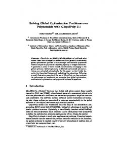
problems, turning on the convex option allows for better performance on problems that are known to be convex, such as the ones considered for this paper. This option affects the initialization of the slack variables and the ordering of the reduced KKT matrix for Cholesky factorization, and it enforces the use of the predictor-corrector algorithm. Further details are provided in [17]. In Tables 1 and 2, we present numerical results from the DIMACS test suite on problems with second-order cone constraints. The first table gives the results of the ratio reformulation models, and the second table gives the results of the variable perturbation models. Note that the scheduling models and nb L2 are not included in Table 2. The reason for this is that the number of nonzeros in the Hessian is very large when there is a second-order cone constraint with a large dimension. Therefore, the variable perturbation is only used for the models where there are many second-order cone constraints, but where the dimension of each constraint is quite small. Also, the variable perturbation approach did not work for nb and nb L2 bessel, so these models are omitted from Table 2, as well. The results provided in the Tables are iteration counts, runtimes (in CPU seconds), optimal value of the objective function, error of the linear constraints given by kAx − bk, and error of the quadratic constraints given by min(eigK(x, K)). The function eigK is from SeDuMi, and its description can be found in [18]. loqo is able to solve all but two of the largest problems in the test suite, with varying degrees of accuracy. In Table 3, we provide a comparison for the runtimes with the state-of-the-art special-purpose solver SeDuMi. For the most part, loqo is slower especially as the problem size grows, but SeDuMi spends considerably more time on the scheduling problems and concludes that it is running into numerical problems at optimality or cannot solve them. The reformulation of the semidefiniteness constraints works and solves many problems from the SDPLib set [3]. However, only 3 of the problems from the DIMACS Challenge test suite (truss5, hinf12, hinf13) are small enough for us to attempt, but these are challenging problems that loqo cannot solve. We will be performing more numerical testing for the reformulation of the semidefiniteness constraints when Version 2.0 of the DIMACS Challenge test suite is released with a wider variety of problems. For the sake of completeness, however, we present numerical

22


Problem Iter Time Optimal Value norm eigK nql30 54 14.07 -9.460348e-01 1.12539e-13 -2.8132e-06 nql60 83 153.37 -9.350402e-01 2.25583e-13 -1.8045e-05 qssp30 23 8.13 -6.496594e+00 4.12790e-11 -1.4218e-05 qssp60 27 91.05 -6.562395e+00 2.93430e-12 -1.0502e-05 nb 78 85.97 -5.070292e-02 2.77775e-12 -5.7397e-13 nb L1 40 40.64 -1.301228e+01 1.99581e-11 -5.1364e-11 nb L2 240 552.17 -1.628972e+00 8.22174e-12 -1.5701e-16 nb L2 bessel 43 49.37 -1.025683e-01 2.22625e-12 -1.0150e-11 50x50.orig 75 17.06 2.667300e+04 2.48493e-13 -1.7303e-05 50x50.scaled 78 20.26 7.852039e+00 3.87081e-11 -3.6797e-08 100x50.orig 115 57.87 1.818899e+05 9.22323e-09 -3.1298e-08 100x50.scaled 92 55.17 6.716503e+01 1.17143e-09 -3.1057e-09 100x100.orig 122 165.22 7.173671e+05 3.50900e-04 -5.7551e-04 100x100.scaled 106 133.73 2.733079e+01 2.31093e-08 -3.3763e-12 200x100.orig 152 521.60 1.413618e+05 7.88213e-07 5.9207e-08 200x100.scaled 253 831.22 5.182778e+01 7.27618e-11 -6.2027e-06 Table 1. Summary of solution results by LOQO (ratio reformulation) for linear and second-order cone constrained problems from the DIMACS Challenge.

Problem Iter Time Optimal Value norm eigK nql30 52 14.59 -9.460348e-01 7.14911e-14 -8.5374e-06 nql60 73 152.21 -9.350402e-01 3.79208e-13 -1.3250e-05 qssp30 38 17.87 -6.496594e+00 5.23019e-11 -4.1926e-06 qssp60 43 171.69 -6.562395e+00 3.23791e-12 -1.6213e-05 nb L1 52 50.65 -1.301228e+01 1.76626e-12 7.1700e-12 Table 2. Summary of solution results by LOQO (variable perturbation) for linear and second-order cone constrained problems from the DIMACS Challenge.

results in Table 4 for problems from the SDPLib set. The measures of error provided in the table are the number of digits of agreement between the primal and dual objectives for the reformulated problem (sf) and the primal and dual feasibility levels (feas).


23

Problem LOQO SeDuMi nql30 14.07 6.99 nql60 153.37 39.16 qssp30 8.13 10.70 qssp60 91.05 134.57 nb 85.97 35.35 nb L1 40.64 364.22 nb L2 552.17 61.55 nb L2 bessel 49.37 23.10 50x50.orig 17.06 36.17 50x50.scaled 20.26 54.73 100x50.orig 57.87 196.43 100x50.scaled 55.17 481.85 100x100.orig 165.22 527.79 100x100.scaled 133.73 * 200x100.orig 521.60 > 4 hrs 200x100.scaled 831.22 > 4 hrs Table 3. Comparison of runtimes for LOQO (ratio reformulation) and SeDuMi. All runtimes are in CPU Seconds. * indicates that SeDuMi was unable to solve this problem.

Problem Variables Constraints iter time sf feas truss1 25 32 30 0.07 9 10−10 truss2 389 464 192 8.33 5 10−5 truss3 118 122 176 3.29 8 10−5 truss4 49 56 39 0.15 12 10−8 truss6 2024 2147 2867 531.97 4 10−4 truss7 537 752 1500 73.14 3 10−4 Table 4. Iteration counts and runtimes for small truss topology problems from the SDPLib test suite.

7. Conclusions. We have thus outlined two approaches for smoothing second-order cone constraints and a reformulation method for expressing semidefiniteness constraints as nonlinear inequalities. As the numerical results show, a general-purpose solver is quite efficient on problems with linear and second-order cone constraints, especially when a perturbation or reformulation approach is used to handle nonsmoothness issues.

24


The variable perturbation seems to work well for problems with small blocks, whereas the ratio reformulation yields a much sparser Hessian for problems with larger blocks and allows them to be solved faster. The reformulation of the semidefiniteness constraints, on the other hand, can be solved by loqo only for small instances. This is due to A(x) and H(x, y) being dense and the fact that they are quite often expensive to evaluate. This is true more so for the Hessian than for the Jacobian. Sparsity can be improved using properties of the dual problem, nonetheless, it is probably best to use a first-order algorithm to solve problems with semidefiniteness constraints. The true strength of our approach is that there are many NLP solvers in the optimization community that can use our reformulations to solve LSS problems. The semidefiniteness constraints require, of course, that the iterates start and stay feasible. A recent paper by Nocedal, et. al. [16] describes their implementation of a step reducing method for in their solver knitro, and we are planning to perform future numerical tests with this solver. References [1] E. Andersen and K. Andersen. The mosek optimization software. EKA Consulting ApS, Denmark. [2] A. Berman and R.J. Plemmons. Nonnegative Matrices in the Mathematical Sciences. Academic Press, 1979. [3] B. Borchers. Sdplib 1.1, a library of semidefinite programming test problems. 1998. [4] S. Burer, R.D.C. Monteiro, and Y. Zhang. Solving semidefinite programs via nonlinear programming part i: Transformations and derivatives. Technical report, TR99-17, Dept. of Computational and Applied Mathematics, Rice University, Houston TX, 1999. [5] S. Burer, R.D.C. Monteiro, and Y. Zhang. Solving semidefinite programs via nonlinear programming part ii: Interior point methods for a subclass of sdps. Technical report, TR99-17, Dept. of Computational and Applied Mathematics, Rice University, Houston TX, 1999. [6] A.V. Fiacco and G.P. McCormick. Nonlinear Programming: Sequential Unconstrainted Minimization Techniques. Research Analysis Corporation, McLean Virginia, 1968. Republished in 1990 by SIAM, Philadelphia. [7] R. Fletcher. A nonlinear programming problem in statistics (educational testing). SIAM J. Sci. Stat. Comput., 2:257–267, 1981. [8] R. Fletcher. Semi-definite matrix constaints in optimization. SIAM J. Control and Optimization, 23(4):493–513, 1985. [9] D. Goldfarb and K. Scheinberg. Stability and efficiency of matrix factorizations in interior-point methods. Conference Presentation, HPOPT IV Workshop, June 16-18, Rotterdam, The Netherlands, 1999. [10] L. Vandenberghe (editors) H. Wolkowicz, R. Saigal. Handbook of Semidefinite Programming. Kluwer Academic Publishers, 2000.


25

[11] S. Homer and R. Peinado. Design and performance of parallel and distributed approximation algorithms for maxcut. Technical report, Boston University, 1995. [12] D.F. Shanno H.Y. Benson and R.J. Vanderbei. Interior-point methods for nonconvex nonlinear programming: Jamming and comparative numerical testing. Technical Report ORFE 00-02, Department of Operations Research and Financial Engineering, Princeton University, 2000. [13] R.S. Martin and J.H. Wilkinson. Symmetric decomposition of positive definite band matrices. Numer. Math., 7:355–361, 1965. [14] Y.E. Nesterov and A.S. Nemirovsky. Self–concordant functions and polynomial–time methods in convex programming. Central Economic and Mathematical Institute, USSR Academy of Science, Moscow, USSR, 1989. [15] M.L. Overton and R.S. Womersley. Second derivatives for optimizing eigenvalues of symmetric matrices. Technical Report 627, Computer Science Department, NYU, New York, 1993. [16] J. Nocedal R. Byrd and R. Waltz. Feasible interior methods using slacks for nonlinear optimization. Technical report, Optimization Technology Center, 2000. [17] D.F. Shanno and R.J. Vanderbei. Interior-point methods for nonconvex nonlinear programming: Orderings and higher-order methods. Math. Prog., 87(2):303–316, 2000. [18] Jos F. Sturm. Using sedumi 1.02: a matlab toolbox for optimization over symmetric cones. Optimization Methods and Software, 11-12:625–653, 1999. [19] R.J. Vanderbei. AMPL models. http://www.sor.princeton.edu/˜rvdb/ampl/nlmodels. [20] R.J. Vanderbei. LOQO user’s manual. Technical Report SOR 92-5, Princeton University, 1992. revised 1995. [21] R.J. Vanderbei. LOQO user’s manual—version 3.10. Optimization Methods and Software, 12:485–514, 1999. [22] R.J. Vanderbei and D.F. Shanno. An interior-point algorithm for nonconvex nonlinear programming. Computational Optimization and Applications, 13:231–252, 1999. [23] R.J. Vanderbei and H. Yurttan. Using LOQO to solve second-order cone programming problems. Technical Report SOR-98-09, Statistics and Operations Research, Princeton University, 1998. [24] J.H. Wilkinson and C. Reinsch. Handbook for Automatic Computation, volume II: Linear Algebra. Springer-Verlag, Berlin-Heidelberg-New York, 1971.

26


Appendix A. The SDP model. function kth_diag; param K; param N{1..K}; param M; param b{1..M} default 0; set C_index{k in 1..K} within {1..N[k], 1..N[k]}; set A_index{k in 1..K, m in 1..M} within {1..N[k], 1..N[k]}; param C{k in 1..K, (i,j) in C_index[k]}; param A{k in 1..K, m in 1..M, (i,j) in A_index[k,m]}; param eps := 1e-6; var X{k in 1..K, i in 1..N[k], j in i..N[k]} := if (i==j) then 1 else 0; var y{1..M} := 1; maximize f: sum {i in 1..M} y[i]*b[i]; subject to lin_cons1{k in 1..K, (i,j) in C_index[k]}: C[k,i,j] sum {m in 1..M: (i,j) in A_index[k,m]} A[k,m,i,j]*y[m] = X[k,i,j]; subject to lin_cons2{k in 1..K, i in 1..N[k], j in i..N[k]: !((i,j) in C_index[k])}: -sum {m in 1..M: (i,j) in A_index[k,m]} A[k,m,i,j]*y[m] = X[k,i,j]; subject to sdp_cons{k in 1..K, kk in 1..N[k]}: kth_diag({i in 1..N[k], j in 1..N[k]: j >= i} X[k,i,j], kk, N[k]) >= eps; option presolve 0; option loqo_options "sdp"; solve;


Hande Y. Benson, Princeton University, Princeton, NJ Robert J. Vanderbei, Princeton University, Princeton, NJ

27