SOLVING NONLINEAR TWO POINT BOUNDARY VALUE ... - UKM?

Journal of Quality Measurement and Analysis Jurnal Pengukuran Kualiti dan Analisis

JQMA 7(1) 2011, 129-140

SOLVING NONLINEAR TWO POINT BOUNDARY VALUE PROBLEM USING TWO STEP DIRECT METHOD (Menyelesaikan Masalah Nilai Sempadan Dua Titik Tak Linear Menggunakan Kaedah Langsung Dua Langkah) PHANG PEI SEE, ZANARIAH ABDUL MAJID & MOHAMED SULEIMAN ABSTRACT In this paper, we present two step direct method of Adams Moulton type (2PDAM4 and 2PDAM5) for solving nonlinear two point boundary value problems (BVPs) directly. The two step direct method will be utilised to obtain a series solution of the initial value problems at two steps simultaneously. These methods will solve the nonlinear second order BVPs by shooting technique using constant step size. Three step iterative method is considered as a procedure for solving the nonlinear equations and the convergence of the shooting technique. Numerical results are given to illustrate the efficiency and performance of the direct method by the shooting technique with root finding via three-step iterative method for solving boundary value problems. The results clearly show that the two step direct method is able to produce good results compared to the existing method. Keywords: Boundary value problem; direct method; shooting technique ABSTRAK Dalam makalah ini, dicadangkan kaedah langsung dua langkah jenis Adams Moulton (2PDAM4 dan 2PDAM5) untuk menyelesaikan masalah nilai sempadan dua titik yang tak linear secara langsung. Kaedah langsung dua langkah digunakan untuk mendapatkan siri penyelesaian bagi masalah nilai awal pada dua titik serentak. Kaedah ini akan menyelesaikan masalah nilai sempadan peringkat kedua tak linear melalui teknik penembakan dengan menggunakan saiz langkah malar. Kaedah lelaran tiga langkah diambil kira sebagai suatu prosedur untuk menyelesaikan persamaan tak linear dan penumpuan teknik penembakan. Hasil berangka diberi untuk menggambarkan kecekapan dan prestasi kaedah langsung yang dicadangkan dengan teknik penembakan melalui kaedah lelaran tiga langkah untuk menyelesaikan masalah nilai sempadan. Keputusan jelas menunjukkan bahawa kaedah langsung dua langkah mampu menghasilkan keputusan yang baik berbanding dengan kaedah yang sedia ada. Kata kunci: Masalah nilai sempadan; kaedah langsung; teknik penembakan

1. Introduction This paper is concerned for solving directly two point boundary value problems of the form as follows:

y   f ( x, y, y ),

a xb

(1)

with boundary conditions

y (a)   ,

y (b)   ,

(2)

Phang Pei See, Zanariah Abdul Majid & Mohamed Suleiman

where a, b,  ,  are the given constants. Two point boundary value problems occur in a wide variety of problems, including the modelling of chemical reactions, the boundary layer theory in fluid mechanics and heat power transmission theory. Since the boundary value problem has wide application in scientific research, therefore faster and accurate numerical solutions of boundary value problem are very importance. A large number of numerical methods is now available in the literature for solving two point boundary value problems such as higher order finite difference methods proposed by Tirmizi & Tezel (2002) and extended Adomian decomposition method presented by Jang (2008). There are two main approaches for the numerical solutions of BVPs: indirect method and direct method. In indirect method, the higher order BVPs can be reduced to the equivalent first order system of equations and then solved using any numerical method. This approach is very well established but it obviously will enlarge the system. Ha (2001) had solved the two point boundary value problem using fourth order Runge-Kutta method via shooting technique. The second order boundary value problem has been reduced to a system of first order equations. Lin (2008) had solved the two point boundary value problem based on interval analysis. While Attili and Syam (2008) had proposed an efficient shooting method for solving two point boundary value problem using the Adomian decomposition method. Jafri et al. (2009) has consider solving directly two point boundary value problem for second order ordinary differential equations using multistep method in term of backward difference formulae. In this paper, we are concerned for solving nonlinear two point boundary value problems (BVPs) directly using direct method of Adams Moulton type. The given equations in (1) will be treated in their original second order form and therefore the requirement of storage is lower. The approach for solving higher order ordinary differential equations directly has been suggested by Suleiman (1989) Majid et al. (2009) and Ismail et al. (2009). The method proposed in Majid et al. (2009) is adapted for solving BVPs by shooting technique. A simple shooting algorithm for the two point BVPs has been proposed by many researches such as Keller (1968), Langford (1977), and Faires and Burden (1998). Newton’s method is considered as a procedure for solving the nonlinear equation. Yun (2008) had proposed a new three step iterative method for solving nonlinear equations and the numerical results shown that the proposed method converge faster than Newton method. In this research, the three step iterative method for nonlinear equations will be implemented to solve the problem. 2. Formulation of the Method

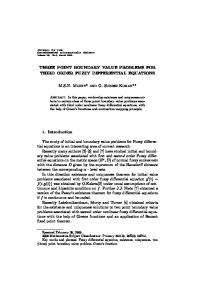
Figure Figure 1: Two Step Direct Method

The interval [a , b] is divided into a series of blocks with each block containing two points as shown in Figure 1. Two approximate values are simultaneously found using the same back values i.e. yn 1 and yn 2 . The first point will be approximated by integrating Eq. (1) over the interval [ xn , xn 1 ] once and twice gives, 130

Solving nonlinear two point boundary value problem using two step direct method



xn1 xn

y( x)dx  

xn1 xn

f ( x, y, y) dx

(3)

and xn1

x

xn

xn

 

y ( x) dxdx  

xn1 xn



x xn

f ( x, y, y ) dxdx.

(4)

The function f ( x, y, y) in Eq. (3) and Eq. (4) will be replaced by Lagrange interpolating polynomial, P . The interpolating points involved in two step direct method of order four (2PDAM4) are ( xn 1 , f n 1 ), ( xn , f n ), ( xn 1 , f n 1 ) and ( xn  2 , f n  2 ) , we will obtain the Lagrange interpolating polynomial: P3 

( x  xn 1 )( x  xn )( x  xn 1 ) f n 2 ( xn  2  xn 1 )( xn  2  xn )( xn  2  xn 1 ) 

( x  xn 1 )( x  xn )( x  xn  2 ) f n 1 ( xn 1  xn 1 )( xn 1  xn )( xn 1  xn  2 )

( x  xn 1 )( x  xn 1 )( x  xn  2 )  fn ( xn  xn 1 )( xn  xn 1 )( xn  xn  2 ) 

(5)

( x  xn )( x  xn 1 )( x  xn 2 ) f n 1 . ( xn 1  xn )( xn 1  xn 1 )( xn 1  xn 2 )

x  xn  2 and by replacing dx  hds and changing the limit of integration from -2 h to -1. Eq. (8) and Eq. (9) can be written as:

Let s 

1

yn 1  yn   P3 hds

(6)

2

1

yn 1  yn  hyn    ( s  1) P3 h 2 ds. 2

(7)

Apply the same process to find the second point, yn  2 of the two step direct method. Eq. (1) will be integrated over the interval [ xn , xn  2 ] once and twice gives,



xn  2 xn

y ( x) dx  

xn  2 xn

f ( x, y, y ) dx

(8)

and xn 2

x

xn

xn

 

y( x) dxdx  

xn 2 xn



x xn

f ( x, y , y )dxdx

(9)

x  xn  2 and by replacing dx  hds and changing the limit of integration from -2 h to 0. Eq. (8) and Eq. (9) can be written as: Let s 

131

Phang Pei See, Zanariah Abdul Majid & Mohamed Suleiman

0

yn  2  yn   P3 hds 2

0

yn  2  yn  hyn    ( s) P3 h 2 ds. 2

(10) (11)

Evaluate these integrals using MAPLE, we obtain the corrector formulae for two step direct method of Adams Moulton type (2PDAM4):

yn 1  yn 

h ( f n 1  13 f n  13 f n 1  f n  2 ) 24

yn 1  yn  hyn 

h2 ( 8 f n 1  129 f n  66 f n 1  7 f n 2 ) 360

h yn  2  yn  ( f n  4 f n 1  f n  2 ) 3 yn  2  yn  2 hyn 

h2 ( 2 f n 1  36 f n  54 f n 1  2 f n  2 ). 45

(12)

(13)

(14)

(15)

The same process is applied to derive the formulae for two step direct method of order five (2PDAM5). The interpolating points involved are ( xn 2 , f n  2 ), ( xn 1 , f n 1 ), ( xn , f n ), ( xn 1 , f n 1 ) and ( xn  2 , f n  2 ) The corrector formulae of 2PDAM5:

yn 1  yn 

h (11 f n 2  74 f n 1  456 f n  346 f n 1  19 f n  2 ) 720

yn 1  yn  hyn 

yn  2  yn 

h2 (11 f n  2  76 f n 1  582 f n  220 f n 1  17 f n  2 ) 1440

h (  f n 2  4 f n 1  24 f n  124 f n 1  29 f n  2 ) 90

yn  2  yn  2 hyn 

h2 ( f n  2  8 f n 1  78 f n  104 f n 1  5 f n  2 ) 90

(16)

(17)

(18)

(19)

This method is the combination of predictor of one order less than the corrector. The same process is applied to find the predictor formulae of the two step direct method. For calculating the initial points, two methods are involved i.e. Euler method and Modified Euler method. These methods will be used at the beginning of the code to find the starting initial points. Both methods will solve the problem directly. Then, the predictor and corrector direct method can be applied until the end of the interval. This direct method will be adapted for solving the boundary value problems via shooting techniques. Shooting technique will allow for new guessing and for each new guessing of the y , the Euler method and Modified Euler method

132

Solving nonlinear two point boundary value problem using two step direct method

will be used again to find the starting initial points. In order to get better approximation for h the initial points when using those methods, the value of h will be reduced to . While the 4 predictor and corrector direct method will remain using the choosing step size h . 3. Implementation of the Method Shooting techniques is an analogy with the procedure of firing objects as a stationary target. It solves the problem with trial and error. To form an initial value problem out of boundary value problem (1), the initial value of y need to be guessed. Starting with the initial guess, s0 , the approximated solution of the derivative y (a ) gives, y   f ( x, y , y ),

a xb

(20) y(a)   ,

y( a )  s0 .

Equation (20) can be written as follows d 2 y ( x, s )  f ( x, y ( x, s ), y ( x, s )) dx 2

(21) y ( a, s )   ,

dy ( a, s)  s. dx

For the first initial guessing, s0 , we considered s0 

  . ba

(22)

See Faires and Burden (1998). The solution of (21) will coincide with the solution of (1) if we could find the value of s  sv such that,

 ( s )  y (b, sv )    0.

(23)

Three step iterative method will be used to get a very rapidly converging iteration. We compute the sv defined as

133

Phang Pei See, Zanariah Abdul Majid & Mohamed Suleiman

Tv  sv 

Uv  

 ( sv )  ( sv )

 (Tv )  (Tv )

sv 1  Tv 

(24)

 ( sv )  (Tv  U v )  .  ( sv )  ( sv )

See Yun (2008) for detail. Differentiate Eq. (21) with respect to s , and it is simplified as follows: z  

d d f ( x, y , y ) z  f ( x, y, y) z  dy dy 

(25) a  x  b,

z (a )  0,

z ( a )  1.

Therefore, the solutions of Eq. (25) will give  ( sv )  z(b, sv ) . The new guess can be calculated base on the previous guess. The three step iterative method will be in the form as follows, Tv  sv 

Uv  

y (b, sv )   z (b, sv )

y (b, Tv )   z (b, sv )

sv 1  Tv 

(26)

y (b, sv )   y (b, Tv  U v )    . z(b, sv ) z(b, sv )

Eq. (26) will give the new estimate for s . The iteration is repeated until we reached the condition | sv 1  sv |  , where  is the prescribed error bound. Both of Eq. (21) and Eq. (25) will be solved simultaneously using the direct two step method. The process is repeated over and over until the error |   y (b, sv ) |  . The algorithms of the proposed method were developed in C language.

134

Solving nonlinear two point boundary value problem using two step direct method

4. Results and Discussion In this section, four numerical examples are presented. The problems will be tested to the direct two step of Adams Moulton method of order four (2PDAM4) and direct two step of Adams Moulton method of order five (2PDAM5). The following notations are used in the tables:

s0 * HA DMS 2PDAM4 2PDAM5

Initial Guess The value end with * is the maximum error Method proposed by Ha (2001) Method proposed by Jafri et al. (2009) Direct two step Adams Moulton method of order four Direct two step Adams Moulton method of order five

Problem 1: y ( x) 

3 2 y , 2

0  x 1

Boundary condition: y (0)  4 , y (1)  1 Exact solution: y ( x) 

4 . (1  x) 2

Source: Ha (2001) Similar with HA and DMS, we chose h  0.05 and used error bound 10 5 . By using the formula stated in (22), we can get the initial guess, s0  3.000 . Ha (2001) did not use formula (22) to obtain the initial guess but the author used s0  0.5 . Table 1 presented the numerical results using s0  3.000 and s0  0.5 . Firstly, a comparison is made between the method of order four, i.e. HA, DMS and 2PDAM4. Table 1 shown that 2PDAM4 is better than DMS and HA for the tested initial guess in term of approximated error and maximum error. The results obtained by 2PDAM5 have better accuracy compare to 2PDAM4 because 2PDAM5 is a method of one order higher than 2PDAM4. The approximate error for the last x at the last iteration is more accurate compare to the other points in the interval because we used three step iterative method to generate the guessing values. In Table 2, the 2PDAM4 and 2PDAM5 methods have less number of iterations compared to HA and DMS when s0  3.0 and s0  0.5 . The final calculating, sv in 2PDAM4 and 2PDAM5 converged to the values of  8.0004 and  8.0001 respectively and the iteration needed is only four for both s0 . In Table 7, 2PDAM4 and 2PDAM5 have reduced the total number of steps almost half compare to HA and DMS method. This result was expected since 2PDAM4 and 2PDAM5 methods approximate the solutions at two points simultaneously.

135

Phang Pei See, Zanariah Abdul Majid & Mohamed Suleiman

Table 1: Comparison of the approximated errors for solving Problem 1

x 0.00 0.10 0.20 0.30 0.40 0.50 0.60 0.70 0.80 0.90 1.00

DMS 0.00 3.19e-4* 2.62e-4 2.11e-4 1.69e-4 1.32e-4 1.01e-4 7.32e-5 4.76e-5 2.34e-5 3.00e-7

s0  3.000 2PDAM4 2PDAM5 0.00 0.00 4.17e-6 1.45e-6* 4.65e-6* 9.97e-7 4.62e-6 8.48e-7 4.31e-6 6.13e-7 3.84e-6 4.53e-7 3.26e-6 3.35e-7 2.58e-6 2.40e-7 1.82e-6 1.57e-7 9.64e-7 7.84e-8 3.89e-16 7.77e-16

HA 0.00 3.0e-6 4.0e-6* 4.0e-6 4.0e-6 4.0e-6 3.0e-6 3.0e-6 3.0e-6 3.0e-6 3.0e-6

s0  0.5 DMS 2PDAM4 0.00 0.00 3.19e-4* 4.17e-6 2.62e-4 4.65e-6* 2.11e-4 4.62e-6 1.68e-4 4.31e-6 1.32e-4 3.84e-6 1.00e-4 3.26e-6 7.21e-5 2.58e-6 4.62e-5 1.82e-6 2.17e-5 9.64e-7 2.40e-7 1.75e-10

2PDAM5 0.00 1.45e-6* 9.97e-7 8.48e-7 6.13e-7 4.53e-7 3.35e-7 2.40e-7 1.57e-7 7.82e-8 1.85e-10

Table 2: The iteration of guess in Problem 1

v

DMS -3.0000 -5.4859 -7.2482 -7.9274 -8.0066 -8.0075 -

1 2 3 4 5 6 7

s0  3.000 2PDAM4 2PDAM5 -3.0000 -3.0000 -7.6423 -7.6419 -8.0004 -8.0001 -8.0004 -8.0001 -

HA 0.5000 -2.7393 -5.5600 -7.3365 -7.9311 -

DMS 0.5000 -1.9756 -4.5634 -6.6849 -7.7767 -7.9997 -8.0075

s0  0.5 2PDAM4 0.5000 -5.4698 -7.9719 -8.0004 -

2PDAM5 0.5000 -5.4615 -7.9712 -8.0001 -

Problem 2:

y ( x)  y 3  yy,

1 x  2

Boundary condition: y (1) 

Exact solution: y( x) 

1 1 , y (2)  2 3

1 . x 1

Source: Ha (2001) This problem was tested using h  0.05 and error bound 105 . By using formulae (22), we obtained the initial guess s0  0.16667 . Ha (2001) did not implement formulae (22) to obtain the initial guess, the author chose s0  4.0 . The numerical results for HA, 2PDAM4 and 2PDAM5 at two different values of initial guess are presented in Table 3 and Table 4. The 2PDAM4 method performs better than HA in term of accuracy. The 2PDAM5 has better accuracy compared to 2PDAM4. Both 2PDAM4 and 2PDAM5 managed to converge the final calculating sv to 0.250000 . In Table 4, the 2PDAM4 and 2PDAM5 methods only took

136

Solving nonlinear two point boundary value problem using two step direct method

three and two iterations to converge while s0  4.0 and 0.16667 respectively. In Table 7, we observed the 2PDAM4 and 2PDAM5 reduced the total steps taken to almost half compared to HA.

Table 3: Comparison of the approximated errors for solving Problem 2

x 1.00 1.10 1.20 1.30 1.40 1.50 1.60 1.70 1.80 1.90 2.00

HA 0.00 5.50e-5 9.10e-5 1.11e-4 1.18e-4* 1.16e-4 1.05e-4 8.80e-5 6.50e-5 3.70e-5 6.00e-6

s 0  4 .0 2PDAM4 0.00 6.02e-9 1.84e-8 3.71e-8 4.63e-8 4.85e-8* 4.58e-8 3.95e-8 3.04e-8 1.93e-8 6.61e-9

2PDAM5 0.00 7.16e-9 1.17e-8 1.19e-8* 1.18e-8 1.09e-8 9.33e-9 7.37e-9 5.12e-9 2.66e-9 5.72e-11

s0  0.16667 2PDAM4 2PDAM5 0.00 0.00 6.03e-9 7.16e-9 1.84e-8 1.17e-8 3.71e-8 1.19e-8* 4.63e-8 1.18e-8 4.86e-8* 1.08e-8 4.59e-8 9.30e-9 3.95e-8 7.33e-9 3.04e-8 5.08e-9 1.93e-8 2.61e-9 6.66e-9 1.92e-13

Table 4: The iteration of guess in Problem 2 s 0  4 .0

v

2PDAM4 4.000000 -0.193056 -0.250000

1 2 3

s0  0.16667 2PDAM4 2PDAM5 -0.166667 -0.166667 -0.250000 -0.250000 -

2PDAM5 4.000000 -0.193118 -0.250000

Problem 3:

y  

32  2 x 3  yy  , 1 x  3 8

Boundary condition: y (1)  17 , y (3)  Exact solution: y  x 2 

43 3

16 x

Source: Ha (2001) Similar with Ha (2001), we tested Problem 3 with h  0.01 , error bound 10 5 and s0  0.25 . Besides that, we also run the numerical result when the initial guess obtain from formula (22), s0  1.33333 . Table 5 shows the approximated error for both initial guess. 2PDAM4 method is more accurate compare to HA at each step. The accuracy of 2PDAM5 method is better compared to 2PDAM4 method. This is expected because the 2PDAM5 method is one order higher than 2PDAM4 method. Table 6 showed that the 2PDAM4 and 2PDAM5 methods managed to converge after three iterations but HA needed 20 iterations to

137

Phang Pei See, Zanariah Abdul Majid & Mohamed Suleiman

converge. In Table 7, 2PDAM4 and 2PDAM5 only need 101 and 102 total steps respectively but HA took 200 total steps.

Table 5: Comparison of the approximated errors for solving Problem 3 x 1.00 1.20 1.40 1.60 1.80 2.00 2.20 2.40 2.60 2.80 3.00

HA 0.0 2.00e-6 3.00e-6 1.00e-6 1.00e-6 0.00e-6 2.00e-6 4.00e-6 6.00e-6 9.00e-6 1.10e-5*

s0  0.25 2PDAM4 0.00 1.88e-8 2.28e-8* 2.09e-8 1.71e-8 1.30e-8 9.14e-9 5.89e-9 3.31e-9 1.37e-9 3.48e-15

2PDAM5 0.00 5.86e-9* 4.03e-9 2.84e-9 1.98e-9 1.35e-9 8.80e-10 5.34e-10 2.86e-10 1.14e-10 3.94e-15

2PDAM4 0.00 1.88e-8 2.28e-8* 2.09e-8 1.71e-8 1.30e-8 9.14e-9 5.89e-9 3.31e-9 1.37e-9 5.91e-15

s0  1.3333 2PDAM5 0.00 5.86e-9* 4.03e-9 2.84e-9 1.98e-9 1.35e-9 8.80e-10 5.34e-10 2.86e-10 1.14e-10 4.75e-15

Table 6: The iteration of guess in Problem 3 v 1 2 3 4 5 6 7 8 9 10 11 12 13 14 15 16 17 18 19 20

HA 0.250000 -25.509144 -15.342037 -13.442387 -14.270104 -13.876993 -14.057735 -13.973262 -14.012450 -13.994210 -14.002692 -13.998731 -14.000594 -13.999723 -14.000119 -13.999936 -14.000038 -13.999974 -14.000022 -13.999996

s0  0.25 2PDAM4 2PDAM5 0.250000 0.250000 -14.017934 -14.017925 -13.999994 -13.999984 -

s0  1.3333

2PDAM4 -1.333333 -14.009589 -13.999994 -

2PDAM5 -1.333333 -14.009580 -13.999984 -

Table 7: The total step for solving Problem 1-3 Method HA DMS 2PDAM4 2PDAM5

138

Problem 1 20 20 11 12

Problem 2 20

Problem 3 200

11 12

101 102

Solving nonlinear two point boundary value problem using two step direct method

Problem 4:

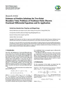
y   e y , 0  x  1 Boundary condition: y (0)  0 , y (1)  0 Source: Lin (2008) We will consider the case with   1 . Figure 2 contains the MATLAB solution, bvp4c together with the approximate solution obtain by 2PDAM4 and 2PDAM5. We could observe the accuracy of the solution obtained in the plot.

Figure

Figure 2: Comparison of the approximate solution for solving Problem 4

5. Conclusion In this paper, we have shown the proposed direct method of Adams Moulton type (2PDAM4 and 2PDAM5) with shooting technique via three-step iterative method using constant step size is suitable for solving two point second order nonlinear boundary value problems. This proposed method is simple, efficient and economically. Acknowledgement The authors gratefully acknowledged the financial support of Research University Grant Scheme (RUGS), project no. 05-03-10-0973RU and Graduate Research Fellowship (GRF) from Universiti Putra Malaysia.

139

Phang Pei See, Zanariah Abdul Majid & Mohamed Suleiman

References Attili B.S. & Syam M.I. 2008. Efficient shooting method for solving two point boundary value problems. Chaos, Solitons and Fractals. 35: 895-903. Faires D. & Burden R.L. 1998. Numerical Methods. 2nd Ed. Pacific Grove: International Thomson Publishing Inc. Ha S. N. 2001. A nonlinear shooting method for two point boundary value problems. Computer and Mathematics with Applications 42: 1411-1420. Ismail F., Ken Y.L. & Othman M. 2009. Explicit and implicit 3-point block methods for solving special second order ordinary differential equations directly. Int. Journal of Math. Analysis 3: 239-254. Jafri M.D., Suleiman M., Majid Z.A. & Ibrahim Z.B. 2009. Solving directly two point boundary value problems using direct multistep method. Sains Malaysiana 38(5): 723-728. Jang B. 2008. Two-point boundary value problems by the extended Adomian decomposition method. Journal of Computations and Applied Mathematics 219: 253-262. Keller H.B. 1968. Numerical methods for Two Point Boundary Value Problems. New York: Blaisdell. Langford W.F. 1977. Shooting algorithm for the best least squares solution of two-point boundary value problems. SIAM J. Numer. Anal. 14(3): 527-542. Lin Y. 2008. Enclosing all solutions of two point boundary value problems for ODEs. Computer and Chemical Engineering 32: 1714-1725. Majid Z.A., Azmi N.A. & Suleiman M. 2009. Solving second order ordinary differential equations using two point four step direct implicit block method. European Journal of Scientific Research 31(1): 29-36. Suleiman M.B. 1989. Solving nonsiff higher order ODEs directly by direct integration method. Applied Mathematics and Computation 33: 197-219. Tirmizi I.A. & Twizell E.H. 2002. Higher-order finite-difference methods for nonlinear second-order two-point boundary value problems. Applied Mathematics Letters 15:897-902. Yun H.Y. 2008. A note on three-step iterative methods for nonlinear equations. Applied Mathematics and Computation 202: 401-405.

Institute for Mathematical Research Universiti Putra Malaysia 43400 UPM Serdang Selangor DE, MALAYSIA E-mail: [email protected]*, [email protected] Mathematics Department Faculty of Science Universiti Putra Malaysia 43400 UPM Serdang Selangor DE, MALAYSIA E-mail: [email protected], [email protected]*, [email protected]

*

Corresponding author

140