Solving Boundary Value Problem for a Nonlinear Stationary ... - arXiv

Solving Boundary Value Problem for a Nonlinear Stationary Controllable System with Synthesizing Control Alexander N. Kvitko, Oksana S. Firyulina and Alexey S. Eremin Faculty of Applied Mathematics and Control Processes, Department of Information Systems, Saint-Petersburg State University, Universitetskii prospekt 35, Petergof, Saint Petersburg, Russia, 198504

An algorithm for constructing a control function that transfers a wide class of stationary nonlinear systems of ordinary differential equations from an initial state to a final state under certain control restrictions is proposed. The algorithm is designed to be convenient for numerical implementation. A constructive criterion of the desired transfer possibility is presented. The problem of an interorbital flight is considered as a test example and it is simulated numerically with the presented method. ‖𝑢‖ < 𝑁.

1. Introduction One of the problems of mathematical control theory is developing of exact or approximate methods to construct control functions and corresponding trajectories, which connect given points in the phase space. A large amount of publications is devoted to researches in this field, for instance [1–12]. Today boundary value problems (BVPs) are quite well studied for linear and non-linear controllable systems of the special form. However the theory of BVPs for general non-linear controllable systems has not yet been sufficiently developed. The main goal of the authors was to construct an algorithm of solving BVPs for a larger class of non-linear controllable systems of ordinary differential equations in the class of synthesizing controls, which would be numerically stable and easy to implement with computer, and to find a constructive sufficient condition of the solution existence for such problems. This goal was reached by reducing the original problem to a linear non-stationary system of a special form and solving the initial value problem for an auxiliary system of ordinary differential equations. The efficiency of the presented algorithm is demonstrated with numerical simulation of a certain practical problem. The object of the study is a controllable system of ordinary differential equations (ODEs) 𝑥̇ = 𝑓(𝑥, 𝑢),

(1.1)

)𝑇

where 𝑥 = (𝑥1 , … , 𝑥𝑛 is a vector of length 𝑛 and 𝑢 is a vector of same or lesser dimension: 𝑢 = (𝑢1 , … , 𝑢𝑟 )𝑇 and 𝑟 ≤ 𝑛. We consider the time to satisfy 𝑡 ∈ [0, 1]. The righthand side 𝑓 ∈ 𝐶 4𝑛 (𝑅𝑛 × 𝑅𝑟 ; 𝑅𝑛 ), 𝑓 = (𝑓1 , … , 𝑓𝑛 )𝑇 ,

(1.2)

𝑓(0, 0) = 0.

(1.3)

With the denotations 𝐴=

𝜕𝑓 𝜕𝑥

(0, 0), 𝐵 =

𝜕𝑓 𝜕𝑢

(0, 0)

rank 𝑆 = 𝑛, 𝑆 = (𝐵, 𝐴𝐵, 𝐴2 𝐵, … , 𝐴𝑛−1 𝐵). We also consider

(1.4)

(1.5)

Problem: To find a pair of functions 𝑥(𝑡) ∈ 𝐶[0, 1] and 𝑢(𝑡) ∈ 𝐶[0, 1] that satisfy (1.1) and the conditions 𝑥(0) = 0 and 𝑥(1) = 𝑥̅ , 𝑥̅ = (𝑥̅1 , … , 𝑥̅𝑛 )𝑇 .

(1.6)

We say that such pair 𝑥(𝑡), 𝑢(𝑡) is a solution of the problem (1.1), (1.6). Theorem. Let the conditions (1.2), (1.3) and (1.4) to be satisfied for the right-hand side of (1.1). Then ∃𝜀 > 0 such that ∀𝑥̅ ∈ 𝑅𝑛 : ‖𝑥̅ ‖ < 𝜀 there exists a solution of the problem (1.1), (1.6), which can be found after solving, first, a problem of stabilizing a linear non-stationary system with exponential coefficients and, second, an initial value problem for an auxiliary ODE system. The main idea of the proof is to use successive changes of independent and dependent variables to reduce the process of solving the original system to the problem of stabilizing a non-linear auxiliary system of ODEs of the special form under constant perturbations. To solve the latter we find a synthesizing control, which provides exponential decrease of the linear auxiliary system fundamental matrix. At the final stage we return to the original variables.

2. Auxiliary system construction We find the function 𝑥(𝑡) being a part of the solution of (1.1), (1.6) in the from 𝑥𝑖 (𝑡) = 𝑎𝑖 (𝑡) + 𝑥̅𝑖 , 𝑖 = 1, … , 𝑛.

(2.1)

In the new variables the system (1.1) and the boundary conditions are written as 𝑎 = 𝑓(𝑥̅ ̇ + 𝑎, 𝑢),

(2.2)

𝑎(0) = −𝑥̅ , 𝑎(1) = 0.

(2.3)

We call a pair of functions 𝑎(𝑡) and 𝑢(𝑡), which satisfy the system (2.2) and the conditions (2.3), a solution of (2.2), (2.3). Consider a problem to find 𝑎(𝑡) ∈ 𝐶[0, 1] and 𝑢(𝑡) ∈ 𝐶[0, 1], which satisfy (2.2), such that

𝑎(0) = −𝑥̅ and 𝑎(𝑡) → 0 as 𝑡 → 1.

(2.4)

Remark 1. The limit with 𝑡 → 1 of the solution of (2.2), (2.4) is the solution of (2.2), (2.3). We make a change of the independent variable 𝑡 in the system (2.2): 𝑡 = 1 − 𝑒 −𝛼𝜏 , 𝜏 ∈ [0, +∞],

(2.5)

𝑐(𝜏) = 𝑎(𝑡(𝜏)), 𝑑(𝜏) = 𝑢(𝑡(𝜏)), 𝑐 = (𝑐1 , … , 𝑐𝑛 )𝑇 , 𝑑 = (𝑑1 , … , 𝑑𝑟 )𝑇 .

We call a pair of functions 𝑐(𝜏) and 𝑑(𝜏), which satisfy the system (2.6) with the conditions (2.7), a solution of the problem (2.6), (2.7). With the solution of (2.6), (2.7) one can restore the solution of (2.2), (2.4) with (2.5) and (2.8). Let’s denote 𝑐̃ = 𝑥̅ + 𝜃𝑖 𝑐, 𝑑̃ = 𝜃𝑖 𝑑, 𝜃 ∈ [0, 1], 𝑖 = 1, … , 𝑛,

where 𝛼 > 0 is a certain constant value to be determined. Then in terms of 𝜏 (2.2) and (2.4) take form: 𝑑𝑐 𝑑𝜏

𝑛

𝑟

|𝑘| = ∑ 𝑘𝑖 ,

|𝑚| = ∑ 𝑚𝑖 ,

𝑖=1

= 𝛼𝑒 −𝛼𝜏 𝑓(𝑥̅ + 𝑐, 𝑑), 𝜏 ∈ [0, +∞],

(2.6)

𝑐(0) = −𝑥̅ , 𝑐(𝜏) → 0 as 𝜏 → ∞,

(2.7)

(2.8)

𝑖=1

𝑘! = 𝑘1 ! ⋅ … ⋅ 𝑘𝑛 !,

𝑚! = 𝑚1 ! ⋅ … ⋅ 𝑚𝑟 !

Using the property (1.2) and Taylor series expansion of the right-hand side of (1.1) about (𝑥̅ , 0), we can rewrite the system (2.6) as:

𝑛

𝑟

𝑗=1 𝑛 𝑟

𝑗=1 𝑟

𝑑𝑐𝑖 𝜕𝑓𝑖 𝜕𝑓𝑖 (𝑥̅ , 0)𝑐𝑗 + 𝛼𝑒 −𝛼𝜏 ∑ (𝑥̅ , 0)𝑑𝑗 = 𝛼𝑒 −𝛼𝜏 𝑓𝑖 (𝑥̅ , 0) + 𝛼𝑒 −𝛼𝜏 ∑ 𝑑𝜏 𝜕𝑥𝑗 𝜕𝑢𝑗 𝑛

𝑛

𝑟

1 𝜕 2 𝑓𝑖 𝜕 2 𝑓𝑖 𝜕 2 𝑓𝑖 (𝑥̅ , 0)𝑐𝑗 𝑐𝑘 + 2 ∑ ∑ (𝑥̅ , 0)𝑐𝑗 𝑑𝑘 + ∑ ∑ (𝑥̅ , 0)𝑑𝑗 𝑑𝑘 ] + 𝛼𝑒 −𝛼𝜏 [∑ ∑ 2 𝜕𝑥𝑗 𝜕𝑥𝑘 𝜕𝑥𝑗 𝜕𝑢𝑘 𝜕𝑢𝑗 𝜕𝑢𝑘 𝑗=1 𝑘=1

+𝛼𝑒 −𝛼𝜏

𝑗=1 𝑘=1

∑ |𝑘|+|𝑚|=4𝑛−2

+𝛼𝑒 −𝛼𝜏

∑ |𝑘|+|𝑚|=4𝑛−1

𝑗=1 𝑘=1

1 𝜕 |𝑘|+|𝑚| 𝑓𝑖 (𝑥̅ , 0) 𝑐1𝑘1 × … × 𝑐𝑛𝑘𝑛 𝑑1𝑚1 × … × 𝑑𝑟𝑚𝑟 𝑘! 𝑚! 𝜕𝑥 𝑘1 … 𝜕𝑥𝑛𝑘𝑛 𝜕𝑢𝑚1 … 𝜕𝑢𝑟𝑚𝑟 1

(2.9)

1

1 𝜕 |𝑘|+|𝑚| 𝑓𝑖 𝑘 𝑘 𝑚 𝑚 (𝑐̃ , 𝑑̃ ) 𝑐1 1 × … × 𝑐𝑛 𝑛 𝑑1 1 × … × 𝑑𝑟 𝑟 , 𝑖 = 1, … , 𝑛. 𝑘! 𝑚! 𝜕𝑥 𝑘1 … 𝜕𝑥𝑛𝑘𝑛 𝜕𝑢𝑚1 … 𝜕𝑢𝑟𝑚𝑟 1

1

Let’s bound the range of 𝑐(𝜏) with ‖𝑐(𝜏)‖ < 𝐶1 , 𝜏 ∈ [0, ∞).

(2.10)

We will now shift the functions 𝑐𝑖 (𝜏), 𝑖 = 1, … , 𝑛, several times. Our aim is to get an equivalent system where all the terms in the right-hand side, which do not contain powers of 𝑐 or 𝑑 in explicit form, would be of the order 𝑂(𝑒 −4𝑛𝛼𝜏 ‖𝑥̅ ‖) as 𝜏 → ∞ and ‖𝑥̅ ‖ → 0 in the area (1.5), (2.10).

(1) At the first stage, we change 𝑐𝑖 (𝜏) to 𝑐𝑖 (𝜏) by the following rule (1)

𝑐𝑖 (𝜏) = 𝑐𝑖 Let 𝐷 |𝑘|+|𝑚| 𝑓𝑖 ≡

𝜕|𝑘|+|𝑚| 𝑓𝑖 𝑘 𝑘 𝑚 𝑚 𝜕𝑥1 1 …𝜕𝑥𝑛𝑛 𝜕𝑢1 1 …𝜕𝑢𝑟 𝑟

(2.11)

for all 𝑖 = 1, … , 𝑛.

After substation of (2.11) into the left- and right-hand sized of (2.9) we obtain the equivalent system

𝑛

(1)

− 𝑒 −𝛼𝜏 𝑓𝑖 (𝑥̅ , 0), 𝑖 = 1, … , 𝑛.

𝑛

𝑛

𝑑𝑐𝑖 𝜕𝑓𝑖 1 𝜕 2 𝑓𝑖 (𝑥̅ , 0)𝑓𝑗 (𝑥̅ , 0) + 𝛼𝑒 −3𝛼𝜏 ∑ ∑ (𝑥̅ , 0)𝑓𝑗 (𝑥̅ , 0)𝑓𝑘 (𝑥̅ , 0) = −𝛼𝑒 −2𝛼𝜏 ∑ 𝑑𝜏 𝜕𝑥𝑗 2 𝜕𝑥𝑗 𝜕𝑥𝑘 𝑗=1

𝑗=1 𝑘=1 𝑛 𝑛

𝑛

+ 𝛼 [𝑒 −𝛼𝜏 ∑ 𝑗=1 𝑟

+ 𝛼 [𝑒 −𝛼𝜏 ∑ 𝑗=1 𝑛

𝜕𝑓𝑖 𝜕 2 𝑓𝑖 (𝑥̅ , 0)𝑐𝑗(1) + 𝑒 −2𝛼𝜏 ∑ ∑ (𝑥̅ , 0)𝑓𝑘 (𝑥̅ , 0)𝑐𝑗(1) ] 𝜕𝑥𝑗 𝜕𝑥𝑗 𝜕𝑥𝑘 𝑗=1 𝑘=1 𝑛 𝑟

𝜕𝑓𝑖 𝜕 2 𝑓𝑖 (𝑥̅ , 0)𝑑𝑘 + 𝑒 −2𝛼𝜏 ∑ ∑ (𝑥̅ , 0)𝑓𝑗 (𝑥̅ , 0)𝑑𝑘 ] 𝜕𝑢𝑗 𝜕𝑥𝑗 𝜕𝑢𝑘 𝑗=1 𝑘=1

𝑛

𝑛

𝑟

1 𝜕 2 𝑓𝑖 𝜕 2 𝑓𝑖 (𝑥̅ , 0)𝑐𝑗(1) 𝑐𝑘(1) + 𝛼𝑒 −𝛼𝜏 ∑ ∑ (𝑥̅ , 0)𝑑𝑘 𝑐𝑗(1) + 𝛼𝑒 −𝛼𝜏 ∑ ∑ 2 𝜕𝑥𝑗 𝜕𝑥𝑘 𝜕𝑥𝑗 𝜕𝑢𝑘 𝑗=1 𝑘=1 𝑟 𝑟

𝑗=1 𝑘=1

1 𝜕 2 𝑓𝑖 (𝑥̅ , 0)𝑑𝑗 𝑑𝑘 + ⋯ + 𝛼𝑒 −𝛼𝜏 ∑ ∑ 2 𝜕𝑢𝑗 𝜕𝑢𝑘 𝑗=1 𝑘=1

+𝛼𝑒

−𝛼𝜏

∑ |𝑘|+|𝑚|=4𝑛−2

𝑘1 1 (1) 𝐷 |𝑘|+|𝑚| 𝑓𝑖 (𝑥̅ , 0) (𝑐1 − 𝑒 −𝛼𝜏 𝑓1 (𝑥̅ , 0)) × … 𝑘! 𝑚! 𝑘𝑛

+𝛼𝑒 −𝛼𝜏

(1) 𝑚 𝑚 × (𝑐𝑛 − 𝑒 −𝛼𝜏 𝑓𝑛 (𝑥̅ , 0)) 𝑑1 1 × … × 𝑑𝑟 𝑟 𝑘1 1 (1) ∑ 𝐷 |𝑘|+|𝑚| 𝑓𝑖 (𝑐̃ , 𝑑̃ ) (𝑐1 − 𝑒 −𝛼𝜏 𝑓1 (𝑥̅ , 0)) × … 𝑘! 𝑚!

|𝑘|+|𝑚|=4𝑛−1

(2.12)

(1)

× (𝑐𝑛 − 𝑒 −𝛼𝜏 𝑓𝑛 (𝑥̅ , 0))

𝑘𝑛

𝑚

𝑚

𝑑1 1 × … × 𝑑𝑟 𝑟 , 𝑖 = 1, … , 𝑛. (1) (2) (2) 𝑐𝑖 (𝜏) = 𝑐𝑖 (𝜏) + 𝑒 −2𝛼𝜏 𝜙𝑖 (𝑥̅ ),

It follows from (2.7) and (2.11) that

𝑛

(1) 𝑐𝑖 (0) = −𝑥̅𝑖 + 𝑓𝑖 (𝑥̅ , 0), 𝑖 = 1, … , 𝑛.

(2) 𝜙𝑖 (𝑥̅ )

(2.13)

𝑛

(2.14)

𝑗=1

It is easy to see that in the right-hand side of (2.12) the terms, which do not contain the powers of the components of 𝑐 or 𝑑 in explicit form, are bounded with 𝑂(𝑒 −2𝛼𝜏 ‖𝑥̅ ‖) as 𝜏 → ∞ and ‖𝑥̅ ‖ → 0 in (1.5), (2.10). At the second stage, we make a change of variables (2)

1 𝜕𝑓𝑖 (𝑥̅ , 0)𝑓𝑗 (𝑥̅ , 0), = ∑ 2 𝜕𝑥𝑗

(2) 𝜙𝑖 (0) = 0, 𝑖 = 1, … , 𝑛.

With respect to these new variables the original system (2.12) and the initial conditions (2.13) are written as:

𝑛

𝑛

𝑑𝑐𝑖 1 𝜕 2 𝑓𝑖 𝜕𝑓𝑖 (𝑥̅ , 0)𝑓𝑗 (𝑥̅ , 0)𝑓𝑘 (𝑥̅ , 0) + 𝑒 −3𝛼𝜏 ∑ (𝑥̅ , 0)𝜙𝑗(2) = 𝛼 [ 𝑒 −3𝛼𝜏 ∑ ∑ 𝑑𝜏 2 𝜕𝑥𝑗 𝜕𝑥𝑘 𝜕𝑥𝑗 𝑗=1 𝑘=1

𝑗=1

𝑛

𝑛

− 𝑒 −4𝛼𝜏 ∑ ∑

+ 𝛼 [𝑒

𝑗=1 𝑘=1 𝑛 𝜕𝑓𝑖 −𝛼𝜏

∑ 𝑗=1

𝜕𝑥𝑗

𝑛

𝑗=1 𝑘=1

𝑛

𝑗=1 𝑘=1 𝑛

+ 𝑒 −3𝛼𝜏 ∑ ∑ 𝑗=1 𝑘=1

+ 𝛼 [𝑒

−𝛼𝜏

𝑛

(𝑥̅ , 0)𝑐𝑗(2) − 𝑒 −2𝛼𝜏 ∑ ∑ 𝑛

𝑛

𝑟

𝑛

𝜕 2 𝑓𝑖 1 𝜕 2 𝑓𝑖 (𝑥̅ , 0)𝑓𝑘 (𝑥̅ , 0)𝜙𝑗(2) + 𝑒 −5𝛼𝜏 ∑ ∑ (𝑥̅ , 0)𝜙𝑗(2) 𝜙𝑘(2) ] 𝜕𝑥𝑗 𝜕𝑥𝑘 2 𝜕𝑥𝑗 𝜕𝑥𝑘 2

𝜕 𝑓𝑖 (𝑥̅ , 0)𝑓𝑘 (𝑥̅ , 0)𝑐𝑗(2) 𝜕𝑥𝑗 𝜕𝑥𝑘

𝜕 2 𝑓𝑖 (𝑥̅ , 0)𝜙𝑘(2) 𝑐𝑗(2) ] 𝜕𝑥𝑗 𝜕𝑥𝑘 𝑛

𝑟

𝑟

𝜕𝑓𝑖 𝜕 2 𝑓𝑖 𝜕 2 𝑓𝑖 (2.15) (𝑥̅ , 0)𝑑𝑘 − 𝑒 −2𝛼𝜏 ∑ ∑ (𝑥̅ , 0)𝑓𝑗 (𝑥̅ , 0)𝑑𝑘 + 𝑒 −3𝛼𝜏 ∑ ∑ (𝑥̅ , 0)𝜙𝑗(2) 𝑑𝑘 ] ∑ 𝜕𝑢𝑗𝑘 𝜕𝑥𝑗 𝜕𝑢𝑘 𝜕𝑥𝑗 𝜕𝑢𝑘

𝑘=1

𝑗=1 𝑘=1

𝑛

𝑛

𝑛

𝑗=1 𝑘=1 𝑟 𝑟

𝑟

1 𝜕 2 𝑓𝑖 𝜕 2 𝑓𝑖 𝜕 2 𝑓𝑖 (𝑥̅ , 0)𝑐𝑗(2) 𝑐𝑘(2) + ∑ ∑ (𝑥̅ , 0)𝑑𝑘 𝑐𝑗(2) + ∑ ∑ (𝑥̅ , 0)𝑑𝑗 𝑑𝑘 ] + 𝛼𝑒 −𝛼𝜏 [∑ ∑ 2 𝜕𝑥𝑗 𝜕𝑥𝑘 𝜕𝑥𝑗 𝜕𝑢𝑘 𝜕𝑢𝑗 𝜕𝑢 𝑗=1 𝑘=1

+𝛼𝑒 −𝛼𝜏

𝑗=1 𝑘=1

∑ |𝑘|+|𝑚|=4𝑛−2

(2)

+𝛼𝑒 −𝛼𝜏

𝑗=1 𝑘=1

𝑘1 1 (2) (2) 𝐷 |𝑘|+|𝑚| 𝑓𝑖 (𝑥̅ , 0) (𝑐1 + 𝑒 −2𝛼𝜏 𝜙1 − 𝑒 −𝛼𝜏 𝑓1 (𝑥̅ , 0)) × … 𝑘! 𝑚! 𝑘𝑛

(2)

𝑚

𝑚

× (𝑐𝑛 + 𝑒 −2𝛼𝜏 𝜙𝑛 − 𝑒 −𝛼𝜏 𝑓𝑛 (𝑥̅ , 0)) 𝑑1 1 × … × 𝑑𝑟 𝑟 𝑘1 1 (2) (2) ∑ 𝐷 |𝑘|+|𝑚| 𝑓𝑖 (𝑐̃ , 𝑑̃ ) (𝑐1 + 𝑒 −2𝛼𝜏 𝜙1 − 𝑒 −𝛼𝜏 𝑓1 (𝑥̅ , 0)) × … 𝑘! 𝑚!

|𝑘|+|𝑚|=4𝑛−1 (2)

(2)

× (𝑐𝑛 + 𝑒 −2𝛼𝜏 𝜙𝑛 − 𝑒 −𝛼𝜏 𝑓𝑛 (𝑥̅ , 0))

𝑘𝑛

𝑚

𝑚

𝑑1 1 × … × 𝑑𝑟 𝑟 , 𝑖 = 1, … , 𝑛.

(2) (2) 𝑐1 (0) = −𝑥̅𝑖 + 𝑓𝑖 (𝑥̅ , 0) − 𝜙𝑖 (𝑥̅ ), 𝑖 = 1, … , 𝑛.

Comparing to the previous variables shift, the right- hand side terms of (2.15), which do not contain the powers of the components of 𝑐 or 𝑑 in explicit form, are now of the order 𝑂(𝑒 −3𝛼𝜏 ‖𝑥̅ ‖) as 𝜏 → ∞ and ‖𝑥̅ ‖ → 0 in the area (1.5), (2.10). By induction, at the 𝑘-th stage, using (2.11)–(2.16) we have the necessary shift of the form: (𝑘−1)

𝑐𝑖

(𝜏) = 𝑐𝑖(𝑘) + 𝑒 −𝑘𝛼𝜏 𝜙𝑖(𝑘) (𝑥̅ ), (𝑘) 𝜙𝑖 (0) = 0, 𝑖 = 1, … , 𝑛.

(2.17)

We apply (2.17) 4𝑛 − 1 times and collect the terms, which are linear in respect to the components of 𝑐 (4𝑛−1) and include the coefficients 𝑒 −𝑖𝛼𝜏 , 𝑖 = 1, … , 𝑛, and also the terms, which are linear in respect to the components of 𝑑 and include the coefficients 𝑒 −𝑖𝛼𝜏 , 𝑖 = 1, … ,2𝑛. Now we have the system, which according to (2.12)–(2.17) can be written in vector form as:

(2.16)

𝑑𝑐 (4𝑛−1) = 𝑃𝑐 (4𝑛−1) + 𝑄𝑑 𝑑𝜏 +𝑅1 (𝑐 (4𝑛−1) , 𝑑, 𝑥̅ , 𝜏) + 𝑅2 (𝑐 (4𝑛−1) , 𝑑, 𝑥̅ , 𝜏) (2.18) +𝑅3 (𝑐 (4𝑛−1) , 𝑑, 𝜏) + 𝑅4 (𝑥̅ , 𝑐 (4𝑛−1) , 𝑑, 𝜏), 𝑅1 = (𝑅11 , . . . , 𝑅1𝑛 )𝑇 , 𝑅2 = (𝑅21 , . . . , 𝑅2𝑛 )𝑇 , 𝑅3 = (𝑅31 , . . . , 𝑅3𝑛 )𝑇 , 𝑅4 = (𝑅41 , . . . , 𝑅4𝑛 )𝑇 . The functions 𝑅1𝑖 consist all the terms which are linear in respect to the components of 𝑐 (4𝑛−1) with coefficients 𝑒 −𝑖𝛼𝜏 , 𝑖 ≥ 𝑛 + 1, and also the terms of the last sum of the right-hand side, for which |𝑚| = 0 and |𝑘| = 1. The functions 𝑅2𝑖 consist all the terms which are linear in respect to the components of 𝑑 with coefficients 𝑒 −𝑖𝛼𝜏 , 𝑖 ≥ 2𝑛 + 1, and also the terms of the last sum of the right-hand side, for which |𝑚| = 1 and |𝑘| = 0. In 𝑅3𝑖 all the terms, which are non-linear in respect of the components of 𝑐 (4𝑛−1) or 𝑑, are contained. Finally, the functions 𝑅4𝑖 include all the terms,

which do not have powers of 𝑐 (4𝑛−1) and 𝑑 components. The functions 𝑃 and 𝑄 have form

Lemma. Let the conditions (1.2) and (1.4) be satisfied for the system (1.1). Then ∃𝜀̅ > 0, 𝜀̅ < 𝜀1 such that ∀𝑥̅ ∈ 𝑅𝑛 : ‖𝑥̅ ‖ < 𝜀̅ there exists a control 𝑑(𝜏) of the form

𝑃(𝑥̅ ) = 𝛼𝑒 −𝛼𝜏 (𝑃1 (𝑥̅ ) + 𝑒 −𝛼𝜏 𝑃2 (𝑥̅ ) + ⋯ + 𝑒 −(𝑛−1)𝛼𝜏 𝑃𝑛−1 (𝑥̅ )), 𝑃1 (𝑥̅ ) =

∂𝑓

(𝑥̅ , 0), 𝑃1 (0) = 𝐴,

∂𝑥

𝑄(𝑥̅ ) = 𝛼𝑒 −𝛼𝜏 (𝑄1 (𝑥̅ ) + 𝑒 −𝛼𝜏 𝑄2 (𝑥̅ ) + ⋯

𝑑 (𝜏) = 𝑀(𝜏)𝑐 (4𝑛−1) (2.19)

+ 𝑒 −(2𝑛−1)𝛼𝜏 𝑄2𝑛−1 (𝑥̅ )), 𝑄1 (𝑥̅ ) =

∂𝑓 ∂𝑢

(𝑥̅ , 0), 𝑄1 (0) = 𝐵.

𝑐 (4𝑛−1) (0) = −𝑥̅ + 𝑓(𝑥̅ ) − 𝜙 (2) (𝑥̅ ) − ⋯ −𝜙 (𝑛−1) (𝑥̅ ), (2.20) (𝑖) (𝑖) 𝑇 (𝑖) 𝜙 = (𝜙1 , . . . , 𝜙𝑛 ) , 𝑖 = 1, . . . ,4𝑛 − 1, 𝜙 (𝑖) (0) = 0.

It follows from the construction of (2.18) that in the area (1.5), (2.10) the following estimations are true ‖𝑃𝑖 (𝑥̅ )‖ → 0, ‖𝑄𝑗 (𝑥̅ )‖ → 0 as ‖𝑥̅ ‖ → 0, 𝑖 = 2, . . . , 𝑛 − 1, 𝑗 = 2, . . . ,2𝑛 − 1;

Proof. We use Krasosvsky linear non-stationary systems 𝑗 stabilization method in the proof. Let 𝐿1 , 𝑗 = 1, . . . , 𝑟, to be the 𝑗-th column of 𝑄. Construct a matrix 𝑆2 = {𝐿11 , 𝐿12 , . . . , 𝐿1𝑘1 , 𝐿21 , . . . , 𝐿2𝑘2 , . . . , 𝐿𝑟1 , . . . , 𝐿𝑟𝑘𝑟 }, 𝑗

𝑗

(3.3)

(3.4)

(4.2)

…, 𝐿𝑟𝑘r are linearly independent. Let’s show that rank 𝑆2 = 𝑛.

(4.3)

Let 𝐿̅1 , 𝑗 = 1, . . . , 𝑟, to be the 𝑗-th column of the matrix −𝛼𝜏 𝛼𝑒 𝑄1 . Consider the matrix 𝑆3 = {𝐿̅11 , 𝐿̅12 , . . . , 𝐿̅1𝑘1 , 𝐿̅21 , . . . , 𝐿̅2𝑘2 , . . . , 𝐿̅𝑟1 , . . . , 𝐿̅𝑟𝑘𝑟 }, ̅𝑗

𝑑𝐿 𝑗 𝑗 𝐿̅𝑖 = 𝛼𝑒 −𝛼𝜏 𝑃1 𝐿̅𝑖−1 − 𝑖−1, 𝑗 = 1, . . . , 𝑟, 𝑖 = 2, . . . , 𝑘𝑗

(4.4)

where 𝑘𝑗 are determined the same way as for 𝑆2 . The conditions (1.2), (2.19) and (3.1) provide that 𝑆2 → 𝑆3 as ‖𝑥̅ ‖ → 0. This lead to the existence of 𝜀2 > 0: 𝜀2 < 𝜀1 such that ∀𝑥̅ ∈ 𝑅𝑛 : ‖𝑥̅ ‖ < 𝜀2 rank 𝑆2 = rank 𝑆3 .

(4.5)

Now, taking in account the Remark 2 and the equality (4.5), we can prove by contradiction that ∀𝑥̅ ∈ 𝑅𝑛 : ‖𝑥̅ ‖ < 𝜀2

∂𝑓

𝑓(𝑥̅ , 0) = (𝜃𝑥̅ , 0)𝑥̅ , 𝜃 = (𝜃1 , … , 𝜃𝑛 )𝑇 , ∂𝑥 𝜃𝑖 ∈ [0,1], 𝑖 = 1, . . . , 𝑛. Remark 2. Let’s denote the 𝑖-th column of the matrix 𝑄1 as 𝑞1𝑖 . Construct a matrix 𝑘 −1 𝑘 −1 {𝑞11 , 𝑃1 𝑞11 , … , 𝑃1 1 𝑞11 ,𝑞12 , 𝑃1 𝑞12 , … , 𝑃1 2 𝑞12 , … 𝑘 −1 … , 𝑞1𝑟 , . . . , 𝑃1 𝑟 𝑞1𝑟 } .

rank 𝑆3 = 𝑛.

𝑘𝑗 −1 𝑗

columns of the form 𝑞1 , . . . , 𝑃1 𝑞1 such that all the 𝑘1 −1 1 𝑘 −1 1 1 2 vectors 𝑞1 , 𝑃1 𝑞1 , …, 𝑃1 𝑞1 , 𝑞1 , 𝑃1 𝑞12 , …, 𝑃1 2 𝑞12, 𝑞1𝑟 , 𝑘𝑟 −1 𝑟 …, 𝑃1 𝑞1 are linearly independent. From the conditions (1.4) and (2.19) it follows, that there exists 𝜀1 > 0 so that rank 𝑆1 = 𝑛 ∀𝑥̅ ∈ 𝑅𝑛 that satisfies ‖𝑥̅ ‖ < 𝜀1 .

‖𝑆2−1 ‖ = 𝑂(𝑒 𝑛𝛼𝜏 ), 𝜏 → ∞.

(3.5)

(4.7)

With use of (4.3), change the variable 𝑐 (4𝑛−1) according to the expression 𝑐 (4𝑛−1) = 𝑆2 (𝜏)𝑦.

(4.8)

As a result we get the system 𝑑𝑦 𝑑𝜏

We now consider the system

(4.6)

From (4.5) and (4.6) it follows that the condition (4.3) is satisfied in the area ‖𝑥̅ ‖ < 𝜀2. Moreover, in that area the structure of 𝑆3 provides the estimation

Here for each 𝑗 = 1, … , 𝑟 𝑘𝑗 is the maximal number of

𝑑𝑐 (4𝑛−1) = 𝑃𝑐 (4𝑛−1) + 𝑄𝑑. 𝑑𝜏

𝑑𝜏

, 𝑗 = 1, . . . , 𝑟, 𝑖 = 2, . . . , 𝑘𝑗 .

Here for each 𝑗 𝑘𝑗 is the maximal number of columns 𝐿1 , 𝑗 …, 𝐿𝑘𝑗 such that the vectors 𝐿11 , 𝐿12 , …, 𝐿1𝑘1 , 𝐿21 , …, 𝐿2𝑘2 , 𝐿𝑟1 ,

The estimation (3.4) follows from the representation

𝑗

𝑑𝐿𝑖−1

𝑑𝜏

Moreover, the conditions (1.2) and (1.3) lead to

𝑆1 =

𝑗

𝐿𝑖 = 𝑃𝐿𝑖−1 −

𝑗

(4𝑛−1) 2

‖𝑅4 (𝑐 (4𝑛−1) , 𝑑, 𝑥̅ , 𝜏)‖ ≤ 𝐿4 ‖𝑥̅ ‖𝑒 −4𝑛𝛼𝜏 , 𝐿4 > 0.

that provides an exponential decrease of the fundamental matrix in (3.5).

(3.1)

‖𝑅1 (𝑐 (4𝑛−1) , 𝑑, 𝑥̅ , 𝜏)‖ ≤ 𝑒 −(𝑛+1)𝛼𝜏 𝐿1 (𝑥̅ )‖𝑐 (4𝑛−1) ‖, ‖𝑅2 (𝑐 (4𝑛−1) , 𝑑, 𝑥̅ , 𝜏)‖ ≤ 𝑒 −(2𝑛+1)𝛼𝜏 𝐿2 (𝑥̅ )‖𝑑‖, 𝐿1 > (3.2) 0, 𝐿2 > 0; ‖ + ‖𝑑‖2 ),

(4.1)

𝑗

3. Right hand side terms evaluation

‖𝑅3 (𝑐 (4𝑛−1) , 𝑑, 𝜏)‖ ≤ 𝑒 −𝛼𝜏 𝐿3 (‖𝑐 𝐿3 > 0.

4. Auxiliary lemma

= 𝑆2−1 (𝑃𝑆2 −

𝑑𝑆2 𝑑𝜏

) 𝑦 + 𝑆2−1 𝑄𝑑.

(4.9)

According to [13] for the first term of the right-hand side of (4.9) we have

𝑑𝑆2 ) = {𝑒̅2 , … , 𝑒̅𝑘1 , 𝜑̅𝑘1 (𝜏), … , 𝑑𝜏 𝑒̅𝑘1+⋯+𝑘𝑟−1+2 , … , 𝑒̅𝑘1+⋯+𝑘𝑟 , 𝜑̅𝑘𝑟 (𝜏)}.

Let

𝑆2−1 (𝑃𝑆2 −

𝑘𝑖

where 𝑒̅𝑖 is a zero vector of size 𝑛 with the only unit at 𝑖-th place, 𝑘𝑗

𝑘

𝜑̅𝑘𝑗 = (−𝜑𝑘11 , . . . , −𝜑𝑘11 , . . . , −𝜑1𝑘𝑗 , . . . , −𝜑𝑘 , 0, . . . ,0) 𝑗

𝑇 𝑛×1

𝑗

and 𝜑𝑘𝑖 𝑗 are the coefficient of 𝐿𝑘𝑗 +1 expansion into the sum of the vectors 𝐿11 , 𝐿12 , …, 𝐿1𝑘1 , 𝐿21 , …, 𝐿2𝑘2 , 𝐿𝑟1 , …, 𝐿𝑟𝑘r , (notice that ∑𝑟𝑗=1 𝑘𝑗 = 𝑛) i.e. 𝑗 𝑗 𝐿𝑘𝑗 +1 = − ∑ 𝜑𝑘𝑖 1 (𝜏)𝐿1𝑖 − ⋯ − ∑ 𝜑𝑘𝑖 𝑗 (𝜏)𝐿𝑖 . (4.10) 𝑖=1

(4.14)

𝑗=1

𝑖 = 1 , . . . , 𝑟, 𝑘

where 𝛾𝑘𝑖 −𝑗 , 𝑗 = 1, . . . , 𝑘𝑖 are chosen so that the 𝜆1𝑘𝑖 , …, 𝜆𝑘𝑖𝑖 of the equations 𝜆𝑘𝑖 + 𝛾𝑘𝑖−1 𝜆𝑘𝑖−1 + ⋯ + 𝛾0 = 0, 𝑖 = 1, … , 𝑟, to satisfy the conditions 𝑗

𝑘𝑗

𝑘1

𝑑𝑖 = ∑(𝜀𝑘𝑖−𝑗 (𝜏) − 𝛾𝑘𝑖−𝑗 )𝜓 (𝑘𝑖 −𝑗) ,

𝑖=1

(4.15)

Due to (4.12), (4.15) and the Remark 3, the control 𝑑𝑖 = 𝛿𝑘𝑖 𝑇𝑘−1 𝑦𝑘𝑖 , 𝑖 = 1, . . . , 𝑟 provides the exponential 𝑖 decrease of the system (4.9) solutions. Switching back to the original variables in (4.14) and using (4.8), we have

The second term is 𝑆2−1 𝑄 = {𝑒̅1 , . . . , 𝑒̅𝑘𝑖+1 , . . . , 𝑒̅𝛾+1 }, 𝛾 = ∑𝑟−1 𝑖=1 𝑘𝑖 .

𝑑𝑖 = 𝛿𝑘𝑖 𝑇𝑘−1 𝑆2 −1 𝑐 (4𝑛−1) , 𝑖 = 1, … , 𝑟, 𝑘 𝑖

Consider the stabilization of the system 𝑑𝑦𝑘𝑖 𝑘 𝑘 𝑘 = {𝑒̅2 𝑖 , … , 𝑒̅𝑘𝑖𝑖 , 𝜑̅𝑘𝑖 } 𝑦𝑘𝑖 + 𝑒̅1 𝑖 𝑑𝑖 , 𝑑𝜏 𝑘 𝑇 𝑦𝑘𝑖 = (𝑦𝑘1𝑖 , . . . , 𝑦𝑘𝑖𝑖 ) , 𝑖 = 1, … , 𝑟,

𝜆𝑖𝑘𝑖 ≠ 𝜆𝑘𝑖 if 𝑖 ≠ 𝑗 and 𝜆𝑖𝑘𝑖 < −(2𝑛 + 1)𝛼 − 1 for 𝑗 = 1, … 𝑘𝑖 , 𝑖 = 1, … 𝑟.

𝑖

(4.16)

(4.11)

where 𝛿𝑘𝑖 = (𝜀𝑘𝑖−1 (𝜏) − 𝛾𝑘𝑖−1 , … , 𝜀0 (𝜏) − 𝛾0 ); 𝑇𝑘𝑖 is the inequality (4.12) matrix, which means that 𝑦𝑘𝑖 = 𝑇𝑘𝑖 𝜓̅, 𝜓̅ =

where 𝑒̅𝑖 𝑖 is a zero vector of size 𝑘𝑖 with the only unit at

(𝜓 (𝑘𝑖−1) , . . . , 𝜓) ; 𝑆2 −1 is the matrix which consists of the 𝑘𝑖 corresponding 𝑘𝑖 rows of 𝑆2−1 . The found control can be written in the form (4.1), where

𝑇

𝑘𝑖 ×1

𝑘

𝑘 𝑖-th place, and 𝜑̅ 𝑘𝑖 = (−𝜑1𝑘𝑖 , … , −𝜑𝑘𝑖𝑖 ) 𝑘 𝑦𝑘𝑖𝑖

𝑇

𝑘𝑖 ×1

.

T

Let = 𝜓. The phase variables of (4.11) are connected to 𝜓(𝜏) and its derivatives with the equalities: 𝑘

𝑘 −1

𝑦𝑘𝑖𝑖 𝑘 −2

𝑦𝑘𝑖𝑖

𝑦𝑘𝑖𝑖 = 𝜓,

𝑘

= 𝜓 (1) + 𝜑𝑘𝑖𝑖 𝜓, 𝑘

𝑘

= 𝜓 (2) + 𝜑𝑘𝑖𝑖 𝜓 (1) + (

𝑑𝜑𝑘𝑖 𝑖

𝑑𝜏

𝑘 −1

+ 𝜑𝑘𝑖𝑖 ) 𝜓, (4.12)

The differentiation of the last equality in (4.12) together with (4.11) leads to (4.13)

The functions 𝑟𝑘𝑖−2 (𝜏), …, 𝑟0 (𝜏), 𝜀𝑘𝑖−1 (𝜏), …, 𝜀0 (𝜏) in (4.12) and (4.13) are linear combinations of the functions 𝜑𝑘𝑖 𝑗 (𝜏), 𝑖 = 1, . . . , 𝑘𝑗 , 𝑗 = 1, . . . , 𝑟 and their derivatives. Remark 3. From the structure of the matrices 𝑃 and 𝑄 it follows (see (2.19) and the representation (4.10)) that the 𝑘 functions 𝜑𝑘𝑖𝑖 (𝜏),…, 𝜑1𝑘𝑖 (𝜏) and their derivatives, as well as 𝑟𝑘𝑖 −2 (𝜏), …, 𝑟0 (𝜏), 𝜀𝑘𝑖−1 (𝜏), …, 𝜀0 (𝜏) are bounded. Other elements of the columns 𝜑̅𝑘𝑗 , 𝑗 = 1, . . . , 𝑟, obey the

𝑟

Denote the fundamental matrix of the system (4.13) closed with the control (4.14) via Ψ(𝜏), (Ψ(0) = 𝐼, an identity matrix). It is obvious that the elements of Ψ(𝜏) are exponential functions of negative argument or their derivatives. Consider the system (3.15) with the control (4.16) 𝑑𝜏

𝑦𝑘1𝑖 = 𝜓 (𝑘𝑖−1) + 𝑟𝑘𝑖−2 (𝜏)𝜓 (𝑘𝑖 −2) + ⋯ + 𝑟1 (𝜏)𝜓 (1) + 𝑟0 (𝜏)𝜓

estimation 𝑂(𝑒 (𝑛−1)𝛼𝜏 ), 𝜏 → ∞.

1

𝑑𝑐 (4𝑛−1)

⋯

𝜓 (𝑘𝑖 ) + 𝜀𝑘𝑖−1 (𝜏)𝜓 (𝑘𝑖 −1) +. . . +𝜀0 (𝜏)𝜓 = 𝑑𝑖 , 𝑖 = 1, . . . , 𝑟.

𝑀(𝜏) = 𝛿𝑘 𝑇𝑘−1 𝑆2 −1 ≡ (𝛿𝑘1 𝑇𝑘−1 𝑆 −1 , . . . , 𝛿𝑘𝑟 𝑇𝑘−1 𝑆 −1 ) . 𝑘 1 2𝑘 𝑟 2𝑘

= 𝐷(𝜏)𝑐 (4𝑛−1) , 𝐷(𝜏) = 𝑃(𝜏) + 𝑄(𝜏)𝑀(𝜏).

(4.17)

Introduce a block-diagonal matrix 𝑇(𝜏). Its diagonal blocks are matrices 𝑇𝑘𝑖 , 𝑖 = 1, . . . , 𝑟. Then, corresponding to (4.8) and (4.12), the fundamental matrix Φ(𝜏), Φ−1 (0) = 𝐼, of the system (4.17) has form Φ(𝜏) = 𝑆2 (𝜏)𝑇(𝜏)Ψ(𝜏)𝑇 −1 (0)𝑆2−1 (0).

(4.18)

The estimation ‖Φ(𝜏)‖ ≤ 𝐾𝑒 −𝛼𝜏 𝑒 −𝜆𝜏 , 𝜆 > 0, 𝐾 > 0

(4.19)

follows from (4.18), the structure of matrices 𝑆2 (𝜏) and Ψ(𝜏) and the Remark 3. Let 𝜀̅ = 𝜀2 . Then the correctness of the Lemma becomes clear from (4.19). Besides, on base of (4.7), (4.16), (4.18) and the Remark 3 we have ‖Φ(𝜏)Φ−1 (𝑡)‖ ≤ 𝐾1 𝑒 −𝜆(𝜏−𝑡) 𝑒 (𝑛−1)𝛼𝑡 ,

(4.20)

𝑡 ≤ 𝜏, 𝜏 ∈ [0, ∞), 𝐾 > 0; ‖𝑀(𝜏)‖ = 𝑂(𝑒 𝑛𝛼𝜏 ), 𝜏 → ∞.

Now, the use (3.2), (3.3), (3.4), (4.1), (5.2) and (5.4) after changing 𝑐 to 𝑧, gives the following estimations in the area (1.5), (2.10) from (5.6) and (5.7):

5. Main theorem proof The system (2.18) with the control (4.16) has form 𝑑𝑐 (4𝑛−1) = 𝐷(𝜏)𝑐 (4𝑛−1) 𝑑𝜏 +𝑅1 (𝑐 (4𝑛−1) , 𝑀(𝜏)𝑐 (4𝑛−1) , 𝑥̅ , 𝜏) +𝑅2 (𝑐 (4𝑛−1) , 𝑀(𝜏)𝑐 (4𝑛−1) , 𝑥̅ , 𝜏) +𝑅3 (𝑐 (4𝑛−1) , 𝑀(𝜏)𝑐 (4𝑛−1) , 𝜏) +𝑅4 (𝑥̅ , 𝑐 (4𝑛−1) , 𝑀(𝜏)𝑐 (4𝑛−1) , 𝜏)

𝜏

+ ∫ 𝑒 −𝛽(𝜏−𝑡) 𝐾1 (𝐿̅𝑒 −𝛼𝑡 ‖𝑧(𝑡)‖ + 𝐿4 ‖𝑥̅ ‖𝑒 −𝛼𝑡 )𝑑𝑡 , 𝜏1

(5.1)

+ ∫ 𝑒 −𝛽(𝜏−𝑡) 𝐾1 (𝐿̅𝑒 −𝛼𝑡 ‖𝑧(𝑡)‖ + 𝐿4 ‖𝑥̅ ‖𝑒 −𝛼𝑡 )𝑑𝑡,

(5.2)

leads to the following representation 𝑑𝑧 = 𝐶(𝜏)𝑧 + 𝑒 3𝑛𝛼𝜏 𝑅1 (𝑒 −3𝑛𝛼𝜏 𝑧, 𝑀(𝜏)𝑒 −3𝑛𝛼𝜏 𝑧, 𝑥̅ , 𝜏) 𝑑𝜏 +𝑒 3𝑛𝛼𝜏 𝑅2 (𝑒 −3𝑛𝛼𝜏 𝑧, 𝑀(𝜏)𝑒 −3𝑛𝛼𝜏 𝑧, 𝑥̅ , 𝜏) (5.3) + 𝑒 3𝑛𝛼𝜏 𝑅3 (𝑒 −3𝑛𝛼𝜏 𝑧, 𝑀(𝜏)𝑒 −3𝑛𝛼𝜏 𝑧, 𝜏) 3𝑛𝛼𝜏 −3𝑛𝛼𝜏 −3𝑛𝛼𝜏 + 𝑒 𝑅4 (𝑥̅ , 𝑒 𝑧, 𝑀(𝜏)𝑒 𝑧, 𝜏). 𝐶(𝜏) = 𝐷(𝜏) + 3𝑛𝛼𝐸. Let’s show that all solutions of (5.3) with initial values (5.2) that start in a sufficiently small neighborhood of zero decrease exponentially. Let Φ1 (𝜏), Φ1−1 (0) = 𝐼, be the 𝑑𝑧 fundamental matrix of the system = 𝐶(𝜏)𝑧. Then on base 𝑑𝜏 of (4.19), (4.20) and (5.2) we have (5.4)

Let’s choose 𝛼 to provide 𝛽 > 0.

(5.5)

The solution of (5.3) with initial values (2.20) can be presented as 𝑧(𝜏) = Φ1 (𝜏)Φ1−1 (𝜏1 )𝑧(𝜏1 ) + 𝜏

𝜏1

(5.6)

The constant 𝐿̅ depends on (1.5), (2.10). We apply the well-known result from [14] to the inequalities (5.8) and (5.9) and obtain ‖𝑧(𝜏)‖ ≤ 𝐾𝑒 −𝜇𝜏 ‖Φ−1 (𝜏1 )𝑧(𝜏1 )‖ 𝜏

+𝐾1 ∫ 𝑒 −𝜇(𝜏−𝑡) 𝐿4 ‖𝑥̅ ‖𝑒 −𝛼𝑡 𝑑𝑡, 𝜏1

for 𝜏 ∈ [𝜏1 , ∞), 𝜇 = 𝛽 − 𝐾1 𝐿̅𝑒 −𝛼𝜏1 ; and ‖𝑧(𝜏)‖ ≤ 𝐾𝑒 −𝜇1𝜏 ‖𝑐 (4𝑛−1) (0)‖

(5.10)

𝜏

+𝐾1 ∫ 𝑒 −𝜇1(𝜏−𝑡) 𝐿4 ‖𝑥̅ ‖𝑒 −𝛼𝑡 𝑑𝑡, 0

for 𝜏 ∈ [0, 𝜏1 ], 𝜇1 = 𝛽 − 𝐾1 𝐿̅. Using (5.5), we fix 𝜏1 > 0 so, that the inequality 𝜇 > 0 is satisfied. Now let’s bound the choice of 𝛼 > 0 with the condition 𝛼 < 𝜇. Then after the integration in the right-hand sides of (5.10) we have ‖𝑧(𝜏)‖ ≤ 𝐾𝑒 −𝜇𝜏 ‖Φ1−1 (𝜏1 )‖‖(𝑧(𝜏1 )‖ + 𝐾2 𝑒 −𝛼𝜏 𝐿4 ‖𝑥̅ ‖, for 𝜏 ∈ [𝜏1 , ∞), and ‖𝑧(𝜏)‖ ≤ 𝐾3 ‖с(4𝑛−1) (0)‖ + 𝐾4 𝐿4 ‖𝑥̅ ‖, for 𝜏 ∈ [0, 𝜏1 ]. Not that all 𝐾𝑖 > 0.

‖𝑧(𝜏)‖ ≤ 𝐾5 𝑒 −𝛼𝜏 ‖𝑥̅ ‖, 𝜏 ∈ [0, ∞), 𝐾5 > 0.

‖𝑑(𝜏)‖ ≤ ‖𝑀(𝜏)‖𝑒 −3𝑛𝛼𝜏 𝐾5 𝑒 −𝛼𝜏 ‖𝑥̅ ‖ ≤ 𝐾6 𝑒 −(2𝑛−1)𝛼𝜏 ‖𝑥̅ ‖, 𝐾6 > 0, for 𝜏 ∈ [0, ∞).

𝜏

∫ Φ1 (𝜏)Φ1−1 (𝑡)𝑒 3𝑛𝛼𝑡 × [𝑅1 𝑧, 𝑀(𝑡)𝑒 −3𝑛𝛼𝑡 𝑧, 𝑥̅ , 𝑡) + −3𝑛𝛼𝑡 (𝑒 𝑅2 𝑧, 𝑀(𝑡)𝑒 −3𝑛𝛼𝑡 𝑧, 𝑥̅ , 𝑡) + 𝑅3 (𝑒 −3𝑛𝛼𝑡 𝑧, 𝑀(𝑡)𝑒 −3𝑛𝛼𝑡 𝑧, 𝑡) + 𝑅4 (𝑥̅ , 𝑒 −3𝑛𝛼𝑡 𝑧, 𝑀(𝑡)𝑒 −3𝑛𝛼𝑡 𝑧, 𝑡)]𝑑𝑡, for 𝜏 ∈ [0, 𝜏1 ).

for 𝜏 ∈ [0, 𝜏1 ), 𝐿̅ > 0.

(5.11)

The constant 𝐾5 depends on the area (1.5), (2.10). With use of (4.1), (4.20), (5.2) and (5.11) we estimate ‖𝑑(𝜏)‖:

𝑧(𝜏) = Φ1 (𝜏)𝑐 (4𝑛−1) (0) +

0 (𝑒 −3𝑛𝛼𝑡

(5.9)

Based on (2.20), (3.4) two last estimations can be written as a single inequality in the area ‖𝑥̅ ‖ < 𝜀̅:

∫ Φ1 (𝜏)Φ1−1 (𝑡)𝑒 3𝑛𝛼𝑡 × [𝑅1 (𝑒 −3𝑛𝛼𝑡 𝑧, 𝑀(𝑡)𝑒 −3𝑛𝛼𝑡 𝑧, 𝑥̅ , 𝑡) + 𝑅2 (𝑒 −3𝑛𝛼𝑡 𝑧, 𝑀(𝑡)𝑒 −3𝑛𝛼𝑡 𝑧, 𝑥̅ , 𝑡) + 𝑅3 (𝑒 −3𝑛𝛼𝑡 𝑧, 𝑀(𝑡)𝑒 −3𝑛𝛼𝑡 𝑧, 𝑡) + 𝑅4 (𝑥̅ , 𝑒 −3𝑛𝛼𝑡 𝑧, 𝑀(𝑡)𝑒 −3𝑛𝛼𝑡 𝑧, 𝑡)]𝑑𝑡, for 𝜏 ∈ [𝜏1 , ∞),

for 𝜏 ∈ [𝜏1 , ∞); and ‖𝑧(𝜏)‖ ≤ 𝐾𝑒 −𝛽𝜏 ‖𝑐 (4𝑛−1) (0)‖

0

‖Φ1 (𝜏)‖ ≤ 𝐾𝑒 −𝛽𝜏 , −1 ‖Φ1 (𝜏)Φ1 (𝑡)‖ ≤ 𝐾1 𝑒 −𝛽(𝜏−𝑡) 𝑒 (𝑛−1)𝛼𝑡 , 𝛽 = 𝜆 − 3𝑛𝛼.

(5.8)

𝜏

Change of the variables 𝑐 (4𝑛−1) = 𝑧𝑒 −3𝑛𝛼𝜏 , 𝑐 (4𝑛−1) (0) = 𝑧(0),

‖𝑧(𝜏)‖ ≤ 𝐾𝑒 −𝛽𝜏 ‖Φ1−1 (𝜏1 )𝑧(𝜏1 )‖

(5.7)

(5.12)

Now we can set the value 𝜀 from the Theorem С 𝑁 formulation, to be min {𝜀̅, 1 , }. This shows that the 𝐾5

𝐾6

solution of the system (5.3) with initial values (5.2), (2.20) doesn’t leave the area ‖𝑧‖ < 𝐶1 for ‖𝑥̅ ‖ < 𝜀 and decreases exponentially. Besides, by (5.12) the corresponding function 𝑑(𝜏) obeys the restriction (1.5). Moreover, if we

substitute the solution to (5.2) and (4.1) and return to the variables 𝑐(𝜏) according to (2.11), (2.14)–(2.17), we get the solution of (2.6), (2.7). Then we write everything in the original variables with (2.8), (2.5) and finally (2.1). Now, according to the Remark 1, passing to the limit as 𝑡 → 1 gives the solution of the original problem (1.1), (1.6). This proves the Theorem. Remark 4. Consider the system 𝑥̇ = 𝑓(𝑥, 𝑢) + 𝐹

(5.13)

where 𝑥 = (𝑥1 , … , 𝑥𝑛 )𝑇 , 𝑥 ∈ 𝑅𝑛 ; 𝑢 = (𝑢1 , … , 𝑢𝑟 )𝑇 , 𝑢 ∈ 𝑅𝑟 ; 𝑡 ∈ [0, 1], 𝑟 ≤ 𝑛, 𝐹 = (𝐹1 , … , 𝐹1 )𝑇 , 𝐹 ∈ 𝑅𝑛 . 𝐹 is a constant perturbation. From the Theorem follows the Corollary. Let the conditions (1.2)–(1.4) to be satisfied for the system (5.13). Then there exists 𝜀 > 0 so that for any 𝑥̅ ∈ 𝑅𝑛 and 𝐹 ∈ 𝑅𝑛 if ‖𝑥̅ ‖ < 𝜀 and ‖𝐹‖ < 𝜀 a solution of (5.13), (1.6) exists and it can be found after stabilizing a linear non-stationary system with exponential coefficients and solving the initial value problem for an auxiliary system of ODEs.

𝑔(𝑐1 , 𝑐3 ) = − and

𝑐𝑖 (0) = −𝑥̅𝑖 , 𝑐𝑖 (𝜏) → 0 as 𝜏 → ∞, 𝑖 = 1, 2, 3.

To demonstrate the effectiveness of the proposed method we consider a problem of transferring a material point moving in a central gravitational field to a desired circular orbit with jet power. According to [12] the system in deviations from the prescribed circular motion and the condition (1.6) take form 𝑥̇1 = 𝑥2 , (𝜒0 + 𝑥3 )2 𝜈 𝑥̇ 2 = − + + 𝑎𝑟 𝑢, (𝑟0 + 𝑥1 )2 (𝑟0 + 𝑥1 )3

In the following we assume 𝑥̅ = (𝑥̅1 , 0, 0)𝑇 . It is necessary to make seven transforms of the type (2.17) to solve the problem (6.3), (6.4): 1

𝑐2 = 𝑧2 − 𝑒 −𝛼𝜏 𝑔(𝑥̅1 ), 𝑐1 = 𝑧1 + 𝑒 −2𝛼𝜏 𝑔(𝑥̅1 ), 2 1 −3𝛼𝜏 𝜕𝑔 (𝑥̅ )𝑔(𝑥̅1 ), 𝑧2 = 𝑤2 − 𝑒 6 𝜕𝑐1 1 1 −4𝛼𝜏 ∂𝑔 (𝑥̅ )𝑔(𝑥̅1 ), 𝑧1 = 𝑤1 + 𝑒 24 ∂c1 1 𝑤2 = 𝜐2 − 𝑒 −5𝛼𝜏 𝑔̅ , 𝑤1 = 𝜐1 + 𝑒 −6𝛼𝜏 𝑔̅̅ , 𝜐2 = 𝑢2 − 𝑒 −7𝛼𝜏 𝑔̅̅ , 2

1 𝜕𝑔 1 𝜕2𝑔 (𝑥̅1 )) 𝑔(𝑥̅1 ) − (𝑥̅ )𝑔2 (𝑥̅1 ), 𝑔̅ = ( 120 𝜕𝑐1 40 𝜕𝑐12 1 2

𝑔̅̅ =

(6.5) 1 𝜕𝑔 1 𝜕2𝑔 2 (𝑥̅ ), (𝑥̅1 )) 𝑔(𝑥̅1 ) + (𝑥̅ )𝑔 ( 1 720 𝜕𝑐1 240 𝜕𝑐12 1

(6.1)

1 1 𝜕𝑔 (𝑥̅ )) 𝑔(𝑥̅1 ) 𝑔̅̅ = { ( 7 720 𝜕𝑐1 1 + +

1 𝜕3𝑔 (𝑥̅ )𝑔3 (𝑥̅1 ) 48 𝜕𝑐13 1 1 𝜕𝑔 𝜕2𝑔 (𝑥̅1 ) 2 (𝑥̅ )𝑔2 (𝑥̅1 )}, 40 𝜕𝑐1 𝜕𝑐1

The matrices 𝑃 and 𝑄 and the system analogous to (3.5), look like 𝑑𝑐̅

= 𝑃𝑐̅ + 𝑄𝑑, 𝑐̅ = (𝜐1 , 𝑢2 , 𝑐3 )𝑇 , 0 1 0 𝑃 = 𝛼𝑒 −𝛼𝜏 ‖𝑎21 0 𝑎23 ‖, 0 0 0 0 −𝛼𝜏 𝑄 = ‖𝛼𝑒 𝑎𝑟 ‖, 𝛼 𝛼𝑒 −𝛼𝜏 𝑏 + 𝑒 −3𝛼𝜏 𝑎𝜓

𝑑𝜏

𝑥̇ 3 = (𝑥1 + 𝑟0 )𝑎𝜓 𝑢, 𝑥𝑖 (0) = 0, 𝑥𝑖 (1) = 𝑥̅𝑖 , 𝑖 = 1, 2, 3.

(6.2) 1

Here 𝑥1 = 𝑟 − 𝑟0 , 𝑥2 = 𝑟̇ , 𝑥3 = 𝜒 − 𝜒0 ; 𝜒0 = (𝜈𝑟0 )2 , 𝑢 = 𝑚̇⁄𝑚; 𝑟0 is the circular orbit radius; 𝑟̇ is the radial velocity; 𝜒 is the generalized momentum; 𝑎𝑟 and 𝑎𝜓 are the relative velocity vector projections onto the radial and tangential directions respectively (they are constant); 𝑚 is the mass and 𝑚̇ is its change rate; 𝜈 = 𝜈 0 𝑀 where 𝜈 0 is the universal gravitational constant; 𝑀 is the mass of the Earth; vector 𝑥 = (𝑥1 , 𝑥1 , 𝑥3 )𝑇 ; and the control 𝑢 ∈ 𝑅1 . The system (2.6) and conditions (2.7) for the problem have form 𝑑𝑐1 = 𝑒 −𝛼𝜏 𝑐2 , 𝑑𝜏

with

(6.4)

3

6. Practical example

𝑑𝑐2 = 𝑒 −𝛼𝜏 𝑔(𝑐1 , 𝑐3 ) + 𝑒 −𝛼𝜏 𝑎𝑟 𝑑, 𝑑𝜏 𝑑𝑐3 = 𝑒 −𝛼𝜏 (𝑐1 + 𝑥̅1 + 𝑟0 )𝑎𝜓 𝑑, 𝑑𝜏

(𝜒0 + 𝑐3 + 𝑥̅3 )2 𝜈 + (𝑟0 + 𝑐1 + 𝑥̅1 )2 (𝑟0 + 𝑐1 + 𝑥̅1 )3

(6.3)

𝑏 = (𝑟0 + 𝑥̅1 )𝑎𝜓 , 𝑎21 =

2 ∂𝑔

∂𝑐1

(𝑥̅1 ), 𝑎23 =

(6.6)

∂𝑔 ∂𝑐3

(𝑥̅1 ).

To stabilize the system (6.6) we construct the matrix 𝑑 {𝐿 𝑆 = 1 , 𝐿2 , 𝐿3 }, with 𝐿1 = 𝑄, 𝐿2 = 𝑃𝐿1 − 𝐿1 , 𝐿3 = 𝑃𝐿2 −

𝑑 𝑑𝜏

𝑑𝜏

𝐿2 , i.e.

0 −𝛼𝜏 𝛼𝑒 𝐿1 = ( ) −𝛼𝜏 (𝑏 𝛼𝑒 + 𝑒 −2𝛼𝜏 𝑔) 𝛼 2 𝑒 −2𝛼𝜏 2 −𝛼𝜏 (𝑒 −𝛼𝜏 −3𝛼𝜏 𝛼 𝑒 𝑎 𝑎23 𝑔 + 1)) 𝐿2 = ( 23 𝑏 + 𝑒 2 −𝛼𝜏 (𝑏 −2𝛼𝜏 𝛼 𝑒 + 3𝑒 𝑔) 𝛼 3𝑒 −2𝛼𝜏 (𝑒 −𝛼𝜏 𝑎23 𝑏 + 𝑒 −3𝛼𝜏 𝑎23 𝑔 + 3) 𝐿3 = (𝛼 3 𝑒 −𝛼𝜏 (𝑒 −2𝛼𝜏 𝑎21 + 3𝑒 −𝛼𝜏 𝑎23 𝑏 + 7𝑒 −3𝛼𝜏 𝑔 + 1)) 𝛼 3 𝑒 −𝛼𝜏 (𝑏 + 9𝑒 −2𝛼𝜏 𝑔) After introducing 𝑐̅ = 𝑆𝑦, 𝑦 = (𝑦1 , 𝑦2 , 𝑦3 )𝑇 we get

𝑑𝑦1 = 𝜑1 (𝜏)𝑦3 + 𝑑, 𝑑𝜏 𝑑𝑦2 = 𝑦1 + 𝜑2 (𝜏)𝑦3 , 𝑑𝜏 𝑑𝑦3 = 𝑦2 + 𝜑3 (𝜏)𝑦3 . 𝑑𝜏

(6.7)

7. Conclusions

The change 𝑦3 = 𝜓(𝜏) reduces (6.7) to a linear equation of the third order 𝜓 (3) − 𝜑3 (𝜏)𝜓 (2) − (2

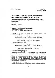
Finally we’ve switched from the auxiliary to the original variables. The plots show the control 𝑢(𝑡) and the corresponding transient plots of the phase coordinates 𝑥1 (𝑡), 𝑥2 (𝑡) and 𝑥(𝑡) in respect of the original independent variable 𝑡.

𝑑𝜑3 + 𝜑2 (𝜏)) 𝜓 (1) 𝑑𝜏

𝑑 2 𝜑3 𝑑𝜑3 −( 2 + + 𝜑1 (𝜏)) 𝜓 = 𝑑. 𝑑𝜏 𝑑𝜏

(6.8)

The analysis of the Theorem proof shows that the most difficult and time-consuming part of the algorithm implementation can be proceeded with analytical methods of computer algebra packages. The results of the numerical simulation of interorbital flight convince that the method can be used for construction and simulation of various technical objects control systems.

The variables 𝑦1 , 𝑦2 and 𝑦3 are connected to 𝜓 (2) , 𝜓 (1) and 𝜓 with 𝑇

𝑦 = 𝑇Ψ, Ψ = (𝜓 (2) , 𝜓 (1) , 𝜓) , 𝑑𝜑3 1 −𝜑3 − ( + 𝜑3 ) 𝑑𝜏 𝑇=‖ ‖. 0 1 −𝜑3 0 0 1 Let 𝑑 = 𝜓 (3) − (6 + 𝜑3 (𝜏))𝜓 (2) − (11 + 2 − (6 +

𝑑𝜑3 + 𝜑2 (𝜏)) 𝜓 (1) 𝑑𝜏

𝑑 2 𝜑3 𝑑𝜑3 + + 𝜑1 (𝜏)) 𝜓. 𝑑𝜏 2 𝑑𝜏

Substituting 𝑑(𝜏) to (6.8) we get the equation with −1, −2 and −3 as roots of the characteristic polynomial. The return to the original variables gives 𝑑 = Γ(𝜏)𝑇 −1 (𝜏)𝑆 −1 (𝜏)𝑐̅, 𝑑𝜑3 Γ = (−(6 + 𝜑3 ), − (11 + 2 + 𝜑2 ) , 𝑑𝜏

FIGURE 1: Time change of the phase variables

(6.9)

𝑑 2 𝜑3 𝑑𝜑2 − (6 + + + 𝜑1 )). 𝑑𝜏 2 𝑑𝜏 It is obvious that (6.9) provides an exponential decrease of (6.6) solutions. At the final stage we solve the initial value problem for the system obtained from (6.3) after changing the phase coordinates according to (6.5) with the control (6.9). Then we return to the original variables. The initial values for the Cauchy problem are 1

1 ∂𝑔

2

24 ∂𝑐1

𝜐1 (0) = −𝑥̅1 − 𝑔(𝑥̅1 ) − 𝑢2 (0) = 𝑔(𝑥̅1 ) +

1 ∂𝑔 6 ∂𝑐1

(𝑥̅1 )𝑔(𝑥̅1 ) − 𝑔̅̅ ,

(𝑥̅1 )𝑔(𝑥̅1 ) + 𝑔̅ + 𝑔̅̅ ,

𝑐3 (0) = 0. During the numerical simulation we have solved the auxiliary system of ODEs constructed from (6.3) and (6.9) after changing the phase coordinates according to (4.5) with the initial values 𝜐1 (0), 𝑢2 (0), 𝑐3 (0) for 𝑥̅1 = 10 meters, 𝑟0 = 7 ⋅ 106 meters, 𝛼 = 0.1 and time span [0; 12.5].

FIGURE 2: Time change of the control 𝑢(𝑡)

References [1] V.I. Zubov, Lektsii po teorii upravleniya [Lectures on Control Theory, Textbook], 2 ed., Lan, Moscow, 2009 (In Russian). [2] V.A .Komarov, “Design of constrained control signals for nonlinear non-autonomous systems,” Automation and Remote Control, vol. 45, no. 10, pp. 1280–1286, 1984. [3] A.P. Krishchenko, “Controllability and attainability sets of nonlinear control systems,” Automation and Remote Control, vol. 45, no. 6, pp. 707–713, 1984. [4] A. Dirk, “Controllability for polynomial systems,” Lecture Notes in Control and Information Sciences, no. 63, pp. 542– 545, 1984. [5] O. Huashu, “On the controllability of nonlinear control system,” Computational Mathematics, vol. 10, no. 6, pp. 441–451, 1985. [6] V.P. Panteleev, “Ob upravlyaemosti nestatsionarnykh lineinykh sistem [Сontrollability of time-dependent linear systems],” Differential Equations, vol. 21, no. 4, pp. 623– 628, 1985 (In Russian). [7] E.D. Sontag, Mathematical Control Theory: Deterministic Finite Dimensional Systems, Springer, New York, 1998. [8] S.A. Aisagaliev, “On the Theory of the Controllability of Linear Systems,” Automation and Remote Control, vol. 52, no. 2, part 1, pp. 163–171, 1991. [9] Yu.I. Berdyshev, “On the construction of the reachability domain in one nonlinear problem,” Journal of Computer and Systems Sciences International, vol. 45, no. 4, pp. 526–531, 2006. [10] A.N. Kvitko, “On one method of solving a boundary problem for a nonlinear nonstationary controllable system taking measurement results into account,” Automation and Remote Control, vol. 73, no. 12, pp. 2021–2037, 2012. [11] A.N. Kvitko, T.S. Taran, and O.S. Firyulina, “Control problem with incomplete information,” in Proceedings of the IEEE International Conference “Stability and Control Processes” in Memory of V.I. Zubov (SCP), pp. 106–109, Saint-Petersburg, Russia, 2015. [12] N.N. Krasovsky, Teoriya upravleniya dvizheniem [Theory of Motion Control], Nauka, Moscow, 1968 (In Russian). [13] E.Ya. Smirnov, Stabilization of programmed motion, CRC Press, 2000. [14] E.A. Barbashin, Introduction to the theory of stability, Wolters-Noordhoff, 1970.