Computer Vision Winter Workshop 2007, Michael Grabner, Helmut Grabner (eds.) St. Lambrecht, Austria, February 6–8 Graz Technical University
Solving polynomial equations for minimal problems in computer vision Zuzana K´ukelov´a and Tom´asˇ Pajdla CMP, Department of Cybernetics, Czech Technical University in Prague, Czech Republic
[email protected],
[email protected] Abstract Many vision tasks require efficient solvers of systems of polynomial equations. Epipolar geometry and relative camera pose computation are tasks which can be formulated as minimal problems which lead to solving systems of algebraic equations. Often, these systems are not trivial and therefore special algorithms have to be designed to achieve numerical robustness and computational efficiency. In this work we suggest improvements of current techniques for solving systems of polynomial equations suitable for some vision problems. We introduce two tricks. The first trick helps to reduce the number of variables and degrees of the equations. The second trick can be used to replace computationally complex construction of Gr¨obner basis by a simpler procedure. We demonstrate benefits of our technique by providing a solution to the problem of estimating radial distortion and epipolar geometry from eight correspondences in two images. Unlike previous algorithms, which were able to solve the problem from nine correspondences only, we enforce the determinant of the fundamental matrix be zero. This leads to a system of eight quadratic and one cubic equation. We provide an efficient and robust solver of this problem. The quality of the solver is demonstrated on synthetic and real data.
1
Introduction
Estimating camera models from image matches is an important problem. It is one of the oldest computer vision problems and even though much has already been solved some questions remain still open. For instance, a number of techniques for modeling and estimating projection models of wide angle lenses appeared recently [6, 17, 9, 26, 27]. Often in this case, the projection is modeled as the perspective projection followed by radial “distortion” in the image plane. Many techniques for estimating radial distortion based on targets [28, 30], plumb lines [1, 4, 12, 25], and multiview constraints [20, 29, 11, 6, 17, 27, 19, 14] have been suggested. The particularly interesting formulation, based on the division model [6], has been introduced by Fitzgibbon. His formulation leads to solving a system of algebraic equations. It is especially nice because the algebraic constraints of the epipolar geometry, det(F) = 0 for an uncalibrated and 2 E E> E − trace(E E> )E = 0 for a calibrated situation [10], can be “naturally” added to the constraints arising from correspondences to reduce the number of points
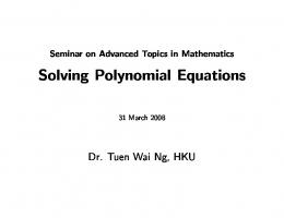
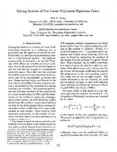
Figure 1: (Left) Image with radial distortion. (Right) Corrected image.
needed for estimating the distortion and the fundamental matrix. A smaller number of the points considerably reduces the number of samples in RANSAC [5, 10]. However, the resulting systems of polynomial equations are more difficult than, e.g., the systems arising from similar problems for estimating epipolar geometry of perspective cameras [23, 22]. In this paper we will solve the problem arising from taking det(F) = 0 constraint into account. Fitzgibbon [6] did not use the algebraic constraints on the fundamental matrix. In fact, he did not explicitly pose his problem as finding a solution to a system of algebraic equations. Thanks to neglecting the constraints, he worked with a very special system of algebraic equations which can be solved numerically by using a quadratic eigenvalue solver. Micusik and Pajdla [17] also neglected the constraints when formulating the estimation of paracatadioptric camera model from image matches as a quartic eigenvalue problem. The work [19] extended Fitzbiggon’s method for any number of views and any number of point correspondences using generalized quadratic eigenvalue problem for rectangular matrices, again without explicitly solving algebraic equations. Li and Hartley [14] treated the original Fitzgibbon’s problem as a system of algebraic equations and used the hidden variable technique [2] to solve them. No algebraic constraint on the fundamental matrix has been used. The resulting technique solves exactly the same problem as [6] but in a different way. Our experiments have shown that the quality of the result was comparable but the technique [14] was considerably slower than the original technique [6]. Work [14] mentioned the possibility of using the algebraic constraint det(F) = 0 to solve for a two parametric model from the same number of points but it did not use it to really solve the problem. Using this constraint makes the problem much harder because the degree of equations involved
1
Solving polynomial equations for minimal problems in computer vision significantly increases. We formulate the problem of estimating the radial distortion from image matches as a system of algebraic equations and by using the constraint det(F) = 0 we get a minimal solution to the autocalibration of radial distortion from eight correspondences in two views. Our work adds a new minimal problem solution to the family of previously developed minimal problems, e.g. the perspective three point problem [5, 8], the five point relative pose problem [18, 22, 15], the six point focal length problem [23, 13], six point generalized camera problem [24]. We follow the general paradigm for solving minimal problems in which a problem is formulated as a set of algebraic equations which need to be solved. Our main contribution is in improving the technique for solving the set of algebraic equations and applying it to solve the minimal problem for the autocalibration of radial distortion. We use the algebraic constraint det(F) = 0 on the fundamental matrix to get an 8-point algorithm. It reduces the number of samples in RANSAC 1.15 (1.45, 2.53) times for 10% (30%, 60%) outliers and is more stable than previously known 9point algorithms [6, 14].
2
Solving algebraic equations
In this section we will introduce the technique we use for solving systems of algebraic equations. We use the nomenclature from excellent monographs [3, 2], where basic concepts from polynomial algebra, algebraic geometry, and solving systems of polynomial equations are explained. Our goal is to solve a system of algebraic equations f1 (x) = ... = fm (x) = 0 which are given by a set of m polynomials F = {f1 , ..., fm | fi ∈ C [x1 , ..., xn ]} in n variables over the field C of complex numbers. We are only interested in systems which have a finite number, say N , solutions and thus m ≥ n. The ideal I generated by polynomials F can be written as (m ) X I= fi pi | pi ∈ C [x1 , ..., xn ] i=1
with f1 , ..., fm being generators of I. The ideal contains all polynomials which can be generated as an algebraic combination of its generators. Therefore, all polynomials from the ideal are zero on the zero set Z = {x|f1 (x) = ... = fm (x) = 0}. In general, an ideal can be generated by many different sets of generators which all share the same solutions. There is a special set of generators though, the reduced Gr¨obner basis G = {g1 , ..., gl } w.r.t. the lexicographic ordering, which generates the ideal I but is easy (often trivial) to solve. Computing this basis and “reading off” the solutions from it is the standard method for solving systems of polynomial equations. Unfortunately, for most computer vision problems this “Gr¨obner basis method w.r.t. the lexicographic ordering” is not feasible because it has double exponential computational complexity in general. To overcome this problem, a Gr¨obner basis G under another ordering, e.g. the graded reverse lexicographical ordering, which is often easier to compute, is constructed. Then,
2
[←]
the properties of the quotient ring A = C [x1 , ..., xn ] /I, i.e. the set of equivalence classes represented by remainders modulo I, can be used to get the solutions. The linear basis of this quotient as B = n ring can be written o α α α αG α {x |x ∈ / hLM (I)i} = x |x = x , where xα is G
αn 1 α2 α is the reminder of xα monomial xα = xα 1 x2 ...xn , x on the division by G, and hLM (I)i is ideal generated by leading monomials of all polynomials form I. In many cases (when I is radical [2]), the dimension of A is equal to the number of solutions N©. Then, the basisªof A consists of N monomials, say B = xα(1) , ..., xα(N ) . Denoting the ba¤T £ sis as b (x) = xα(1) ...xα(N ) , every polynomial q (x) ∈ T A can be expressed as q (x) = b (x) c, where c is a coefficient vector. The multiplication by a fixed polynomial f (x) (a polynomial in variables x = (x1 , ..., xn )) in the quotient ring A then corresponds to a linear operator Tf : A → A which can be described by a N × N action matrix Mf . The solutions to the set of equations can be read off directly from the eigenvalues and eigenvectors of the action matrices. We have ³ ´ ³ ´ T T f (x) q (x) = f (x) b (x) c = f (x) b (x) c
Using properties of the action matrix Mf , we obtain ³ ´ T T f (x) b (x) c = b (x) Mf c, Each polynomial t ∈ C [x1 , ..., xn ] can be written in the Pl form t = i=1 hi gi + r, where gi are basis vectors gi ∈ G = {g1 , ..., gl } , hi ∈ C [x1 , ..., xn ] and r is the reminder of t on the division by G. If p = (p1 , ..., pn ) is a solution to our system of equations, then we can write l ³ ´ X T f (p) q (p) = f (p) b (p) c = hi (p) gi (p) + r (p) i=1
where r (p) is the reminder of f (p) q (p) on the division by Pl G. Because gi (p) = 0 for all i = 1, ..., l we have i=1 hi (p) gi (p) + r (p) = r (p) and therefore ³ ´ ³ ´ G T T f (p) b (p) c = r (p) = f (p) b (p) c . Thus, for a solution p, we have ³ ´ G ³ ´ T T T f (p) b (p) c = f (p) b (p) c = b (p) Mf c for all c, and therefore T
T
f (p) b (p) = b (p) Mf . Therefore, if p = (p1 , ..., pn ) is a solution to our system of equations and f (x) is chosen such that the values f (p) are distinct for all p, the N left eigenvectors of the action matrix Mf are of the form iT h v = βb (p) = β pα(1) ...pα(N ) , for some β ∈ C , β 6= 0. Thus action matrix Mf of the linear operator Tf : A → A of the multiplication by a suitably chosen polynomial f w.r.t. the basis B of A can be constructed and then the solutions to the set of equations can be read off directly from the eigenvalues and eigenvectors of this action matrix [2].
Zuzana K´ukelov´a and Tom´asˇ Pajdla 2.1
Simplifying equations by lifting
The complexity of computing an action matrix depends on the complexity of polynomials (degree, number of variables, form, etc.). It is better to have the degrees as well as the number of variables low. Often, original generators F may be transformed into new generators with lower degrees and fewer variables. Next we describe a particular transformation method—lifting method—which proved to be useful. Assume m polynomial equations in l monomials. The main idea is to consider each monomial that appears in the system of polynomial equations as an unknown. In this way, the initial system of polynomial equations of arbitrary degree becomes linear in the new “monomial unknowns”. Such system can by written in a matrix form as
[←] in [23, 21, 22] for computing Gr¨obner bases but we retrieve the basis B and polynomials required for constructing the action matrix instead. Having B, the action matrix can be computed as follows. If for some xα(i) ∈ B and chosen f , f xα(i) ∈ A, then ¡ ¢ G Tf xα(i) = f xα(i) = f xα(i) and we are done. For all other xα(i) ∈ B for which f xα(i) ∈ / A consider polynomials qi = f xα(i) + hi from I with hi ∈ A. For these xα(i) , ¡ ¢ G G Tf xα(i) = f xα(i) = qi − hi = −hi ∈ A. Since polynomials qi are from the ideal I, we can generate them as algebraic PN combinations of the initial generators F . Write hi = j=1 cji xα(j) for some cji ∈ C, i = 1, ..., N . Then the action matrix Mf has the form 0 B B B Mf = B B B @
MX = 0
c11 c21 . . . cN 1
c12 .
.
.
.
. .
c1N . . . . cN N
1 C C C C. C C A
where X is a vector of l monomials and M is a m × l coefficient matrix. If m < l, then a basis of m − l dimensional null space of matrix M can be found and all monomial unknowns can be expressed as linear combinations of basic vectors of the null space. The coefficients of this linear combination of basic vectors become new unknowns of the new system which is formed by utilizing algebraic dependencies between monomials. In this way we obtain a system of polynomial equations in new variables. The new set of variables consists of unknown coefficients of linear combination of basic vectors and of old unknowns which we need for utilizing dependencies between monomials. The new system is equivalent to the original system of polynomial equations but may be simpler. This abstract description will be made more concrete in Section 3.1.
To get this action matrix Mf , it suffice to generate polynomiPN als qi = f xα(i) + j=1 cji xα(j) from the initial generators F for all these xα(i) ∈ B. This in general seems to be as difficult as generating the Gr¨obner basis but we shall see that it is quite simple for the problem of calibrating radial distortion which we describe in the next section. It is possible to generate qi ’s by starting with F and systematically generating new polynomials by multiplying them by individual variables and reducing them by the Gauss-Jordan elimination. This technique is a variation of the F4 algorithm for constructing Gr¨obner bases [7] and seems to be applicable to more vision problems. We are currently investigating it and will report more results elsewhere.
2.2
2.3
Constructing action matrix efficiently
The standard method for computing action matrices requires to construct a complete Gr¨obner basis and the linear basis ¡ ¢ G B of the algebra A and ©to compute Tf xªα(i) = f xα(i) for all xα(i) ∈ B = xα(1) , ..., xα(N ) [2]. Note that α (i) α (i) α (i) xα(i) = x1 1 x2 2 ...xnn . For some problems, however, it may be very expensive to find a complete Gr¨obner basis. Fortunately, to compute Mf we do not always need a complete Gr¨obner basis. Here we propose a method for constructing the action matrix assuming that the monomial basis B of algebra A is known or can be computed for a class of problems in advance. Many minimal problems in computer vision have the convenient property that the monomials which appear in the set of initial generators F are always same irrespectively from the concrete coefficients arising from non-degenerate image measurements. For instance, when computing the essential matrix from five points, we need to have five linear, linearly independent, equations in elements of E and ten higher order algebraic equations 2 E E> E − trace(E E> ) E = 0 and det(E) = 0 which do not depend on particular measurements. Therefore, the leading monomials of the corresponding Gr¨obner basis, and thus the monomials in the basis B are always the same. They can be found once in advance. To do so, we use the approach originally suggested
. cN 2
The solver
The algorithmic description of our solver of polynomial equations is as follows. 1. Assume a set F = {f1 , ..., fm } of polynomial equations. 2. Use the lifting to simplify the original set of polynomial equations if possible. Otherwise use the original set. 3. Fix a monomial ordering (The graded reverse lexicographical ordering is often good). 4. Use Macaulay 2 [21] to find the basis B as the basis which repeatedly appears for many different choices of random coefficients. Do computations in a suitably chosen finite field to speed them up. 5. For suitably chosen polynomial f construct the polynomials qi by systematically generating higher order polynomials from generators F . Stop when all qi ’s are found. Then construct the action matrix Mf . 6. Solve the equations by finding eigenvectors of the action matrix. If the initial system of equations was transformed, extract the solutions to the original problem. This method extends the Gr¨obner basis method proposed in [23, 21] (i) by using lifting to simplify the problem and (ii) by constructing the action matrix without constructing a
3
Solving polynomial equations for minimal problems in computer vision complete Gr¨obner basis. This brings an important advantage for some problems. Next we will demonstrate it by showing how to solve the minimal problem for correcting radial distortion from eight point correspondences in two views.
3
A minimal solution for radial distortion
We want to correct radial lens distortion using the minimal number of image point correspondences in two views. We assume one-parameter division distortion model [6]. It is well known that for standard uncalibrated case without considering radial distortion, 7 point correspondences are sufficient and necessary to estimate the epipolar geometry. We have one more parameter, the radial distortion parameter λ. Therefore, we will need 8 point correspondences to estimate λ and the epipolar geometry. To get this “8-point algorithm”, we have to use the singularity of the fundamental matrix F. We obtain 9 equations in 10 unknowns by taking equations from the epipolar constraint for 8 point correspondences p> ui
(λ) F p0ui
(λ) = 0,
then mi = (xd x0d , xd yd0 , xd , yd x0d , yd yd0 , yd , x0d , yd0 , 1, xd rd02 , xyd rd02 , rd2 x0d , rd2 yd0 , rd2 + rd02 , rd2 rd02 ). We obtain 8 linear equations in 15 unknowns. So, in general we can find 7 dimensional null-space. We write X = x1 N1 +x2 N2 +x3 N3 +x4 N4 +x5 N5 +x6 N6 +x7 N7 where N1 , ..., N7 ∈ R15×1 are basic vectors of the null space and x1 , . . . , x7 are coefficients of the linear combination of the basic vectors. Assuming x7 6= 0, we can set x7 = 1. Then we can write X=
p0u
where (λ) , pu (λ) represent homogeneous coordinates of a pair of undistorted image correspondences. The one-parameter division model is given by the formula pu ∼ pd /(1 + λrd2 ) where λ is the distortion parameter, pu = (xu , yu , 1), resp. pd = (xd , yd , 1), are the corresponding undistorted, resp. distorted, image points, and rd is the radius of pd w.r.t. the distortion center. We assume that the distortion center has been found, e.g., by [9]. We also assume square pixels, i.e. rd2 = x2d + yd2 . To use the standard notation, we write the division model as xd 0 xu x + λz = yd + λ 0 ∼ yu . 1 rd2 1 Reducing 9 to 7 unknowns by lifting
We simplify the original set of equations by lifting. The epipolar constraint gives 8 equations with 15 monomials (nine 1st order, five 2nd order, one 3rd order) T
(xi + λzi ) F (x0i + λzi0 ) = 0, i = 1, ..., 8 ¡ ¢ xTi Fx0i + λ xTi Fzi0 + ziT Fx0i + λ2 ziT Fzi0 = 0, i = 1, ..., 8 f1 f2 f3 F = f4 f5 f6 f7 f8 f9 We consider each monomial as an unknown and obtain 8 homogeneous equations linear in the new 15 monomial unknowns. These equation can be written in a matrix form MX = 0
7 X
xi Ni =
i=1
Xj = det (F) = 0,
4
where X = (f1 , f2 , f3 , f4 , f5 , f6 , f7 , f8 , f9 , λf3 , λf6 , λf7 , λf8 , λf9 , λ2 f9 , )T and M is the coefficient matrix. If we denote the i-th row of the matrix M as mi and write xd 0 xi + λzi = yd + λ 0 , 1 rd2
i = 1, . . . , 8
and the singularity of F
3.1
[←]
6 X
6 X
xi Ni + N7
i=1
xi Nij + N7j ,
j = 1, .., 15
i=1
Considering dependencies between monomials and det (F) = 0 we get 7 equations for 7 unknowns x1 , x2 , x3 , x4 , x5 , x6 , λ : X10 = λ.X3 ⇒ X11 = λ.X6 ⇒ X12 = λ.X7 ⇒ X13 = λ.X8 ⇒ X14 = λ.X9 ⇒ X15 = λ.X14 ⇒
6 X i=1 6 X i=1 6 X i=1 6 X i=1 6 X
xi Ni,10 + N7,10 = λ xi Ni,11 + N7,11 = λ xi Ni,12 + N7,12 = λ xi Ni,13 + N7,13 = λ xi Ni,14 + N7,14 = λ
6 X i=1 6 X i=1 6 X i=1 6 X i=1 6 X
i=1 6 X
i=1 6 X
i=1
i=1
xi Ni,15 + N7,15 = λ 0
X1 det (F) = 0 ⇒ det @ X4 X7
X2 X5 X8
xi Ni,3 + N7,3 xi Ni,6 + N7,6 xi Ni,7 + N7,7 xi Ni,8 + N7,8 xi Ni,9 + N7,9
xi Ni,14 + N7,14 1
X3 X6 A = 0 X9
This set of equations is equivalent to the initial system of polynomial equations but it is simpler because instead of eight quadratic and one cubic equation in 9 unknowns (assuming f9 = 1) we have only 7 equations (six quadratic and one cubic) in 7 unknowns. We will use these 7 equations to create the action matrix for the polynomial f = λ. 3.2 Computing B and the number of solutions To compute B, we solve our problem in a random finite prime field Zp (Z/ hpi) with p >> 7, where exact arithmetic can be used and numbers can be represented in a simple and efficient way. It speeds up computations and minimizes memory requirements.
Zuzana K´ukelov´a and Tom´asˇ Pajdla We use algebraic geometric software Macaulay 2, which can compute in finite fields, to solve the polynomial equations for many random coefficients from Zp , to compute the number of solutions, the Gr¨obner basis, and the basis B. If the basis B remains stable for many different random coefficients, it is generically equivalent to the basis of the original system of polynomial equations. We can use the Gr¨obner basis and the basis B computed for random coefficients from Zp thanks to the fact that in our class of problems the way of computing the Gr¨obner basis is always the same and for particular data these Gr¨obner bases differ only in coefficients. This holds for B, which consists of the same monomials, as well. Also, the way of obtaining polynomials that are necessary to create the action matrix is always the same and for a general data the generated polynomials differ again only in their coefficients. This way we have found that our problem has 16 solutions. To create the action matrix, we use the graded reverse lexicographic ordering with x1 > x2 > x3 > x4 > x5 > λ > x6 . With this ordering, we get the basis B = (x36 , λ2 , x1 x6 , x2 x6 , x3 x6 , x4 x6 , x5 x6 , x26 , x1 , x2 , x3 , x4 , x5 , λ, x6 , 1) of the algebra A = C [x1 , x2 , x3 , x4 , x5 , λ, x6 ]/I which, as we shall see later, is suitable for finding the action matrix Mλ . 3.2.1 Computing the number of solutions and basis B Here we show the program for computing the number of solutions and basis B of our problem in Macaulay 2. Similar programs can be used to compute the number of solutions and basis of the algebra A for other problems. // polynomial ring with coeffs from Z30097 R = ZZ/30097[x 1..x 9, MonomialOrder=>Lex]; // Formulate the problem over Zp => the set of equations eq (known variables -> random numbers from Zp ) F = matrix({{x 1,x 2,x 3},{x 4,x 5,x 6}, {x 7,x 8,1 R}}); X1 = matrix{apply(8,i->(random(Rˆ2,Rˆ1)))} ||matrix({{1 R,1 R,1 R,1 R,1 R,1 R,1 R,1 R}}); Z1 = matrix({{0 R,0 R,0 R,0 R,0 R,0 R,0 R,0 R}}) ||matrix({{0 R,0 R,0 R,0 R,0 R,0 R,0 R,0 R}}) ||matrix{apply(8,i->X1 (0,i)ˆ2+X1 (1,i)ˆ2)}; X2 = matrix{apply(8,i->(random(Rˆ2,Rˆ1)))} ||matrix({{1 R,1 R,1 R,1 R,1 R,1 R,1 R,1 R}});
[←] degree I1 //the number of solutions (the number of points in V(I)) transpose gens gb I1 // Groebner basis //the quotient ring A=ZZ/30097[x 1..x 9]/I1 A = R/I1 B = basis A //the basis of the quotient ring A
The above program in Macaulay 2 gives not only the number of solutions and the basis B of the algebra A, but also the information like how difficult it is to compute the Gr¨obner basis, and how many and which S-polynomials have to be generated. The level of verbosity is controlled with the command gbTrace(n). For example for n=0 no extra information is produced and for n=100 we get which S-polynomials were computed, from which polynomials were these Spolynomials created, which S-polynomial did not reduce to 0, which were inserted into the basis and so on. 3.3 Constructing action matrix Here we construct the action matrix Mλ for multiplication by polynomial f = λ. The method described in Section for generating polynomials qi = λxα(i) + PN 2.2 calls α(j) ∈ I. j=1 cji x In graded orderings, the leading monomials of qi are λxα(i) . Therefore, to find qi , it is enough to generate at least one polynomial in the required form for each leading monomial λxα(i) . This can be, for instance, done by systematically generating polynomials of I with ascending leading monomials and testing them. We stop when all necessary polynomials qi are obtained. Let d be the degree of the highest degree polynomial from initial generators F . Then we can generate polynomials qi from F in this way: 1. Generate all monomial multiples xα fi of degree ≤ d. 2. Write the polynomial equations in the form MX = 0, where M is the coefficient matrix and X is the vector of all monomials ordered by the used monomial ordering. 3. Simplify matrix M by the Gauss-Jordan (G-J) elimination. 4. If all necessary polynomials qi have been generated, stop. 5. If no new polynomials with degree < d were generated by G-J elimination, set d = d + 1. 6. Go to 1.
Z2 = matrix({{0 R,0 R,0 R,0 R,0 R,0 R,0 R,0 R}}) ||matrix({{0 R,0 R,0 R,0 R,0 R,0 R,0 R,0 R}}) ||matrix{apply(8,i->X2 (0,i)ˆ2+X2 (1,i)ˆ2)};
In this way we can systematically generate all necessary polynomials. Unfortunately, we also generate many unnecessary polynomials. We use Macaulay 2 to identify the unP1 = X1 + x 9*Z1; necessary polynomials and avoid generating them. P2 = X2 + x 9*Z2; In the process of creating the action matrix Mλ , we repreeq = apply(8, i->(transpose(P1 [i]))*F*(P2 [i])); sent polynomials by rows of the matrix of their coefficients. Columns of this matrix are ordered according to the mono// Ideal generated by polynomials eq + the polynomial det(F) mial ordering. The basic steps of generating the polynomials necessary for constructing the action matrix are as follows: I1 = ideal(eq) + ideal det F; // Compute the number of solutions gbTrace 100 dim I1 //the dimension of ideal I (zero-dimensional ideal ⇐⇒ V(I) is a finite set
(0)
(0)
1. We begin with six 2nd degree polynomials f1 , . . . , f6 (0) and one 3rd degree polynomial f7 = det (F) = 0. We perform G-J elimination of the matrix representing the six 2nd degree polynomials and reconstruct the six re(1) (1) duced polynomials f1 , . . . , f6 .
5
Solving polynomial equations for minimal problems in computer vision (1)
(1)
2. We multiply f1 , . . . , f6 by 1, x1 , x2 , x3 , x4 , x5 , λ, x6 (0) and add f7 to get 49 2nd and 3rd degree polynomials (2) (2) f1 , . . . , f49 . They can be represented by 119 monomials and a 49×119 matrix with rank 49, which we simplify by one G-J elimination again. 3. We obtain 15 new 2nd degree polynomials (2) (2) (f29 . . . , f43 ), six old 2nd degree polynomials (re(1) (1) (2) (2) duced polynomials f1 , . . . , f6 , now f44 . . . , f49 ) and 28 polynomials of degree three. In order to avoid adding 4th degree polynomials on this stage we add only x1 , x2 , x3 , x4 , x5 , λ, x6 multiples of these 15 new 2nd (2) (2) degree polynomials to the polynomials f1 , . . . , f49 . (3) (3) Thus obtaining 154 polynomials f1 , . . . , f154 representable by a 154 × 119 matrix, which has rank 99. We (4) (4) simplify it by G-J elimination and obtain f1 , . . . , f99 . 4. The only 4th degree polynomial that we need is a polynomial in the form λx36 + h, h ∈ A. To obtain this polynomial, we only need to add monomial multiples of (4) (4) one polynomial g from f1 , ..., f99 which has leading 2 monomial LM (g) = λ x6 . This is possible thanks to (4) (4) our monomial ordering. All polynomials f1 , ..., f99 and x1 , x2 , x3 , x4 , x5 , λ, x6 multiples of the 3rd degree polynomial g with LM (g) = λ x26 give 106 polynomials (5) (5) f1 , ..., f106 which can be represented by a 106 × 126 matrix of rank 106. After another G-J elimination, we (6) (6) get 106 reduced polynomials f1 , ..., f106 . Because the polynomial g with LM (g) = λ x26 has already been (2) (2) between the polynomials f1 , ..., f49 , we can add its monomial multiples already in the 3rd step. After one G-J elimination we get the same 106 polynomials. In this way, we obtain polynomial q with LM (q) = λ x36 as q = λ x36 + c1 x2 x26 + c2 x3 x26 + c3 x4 x26 + c4 x5 x26 + h0 , for some c1 , ..., c4 ∈ C and h0 ∈ A instead of the desired λ x36 + h, h ∈ A. (6)
(6)
5. Among the polynomials f1 , ..., f106 , there are 12 out of the 14 polynomials that are required for constructing the action matrix. The first polynomial which is missing is the above mentioned polynomial q1 = λ x36 + h1 , h1 ∈ A. To obtain this polynomial from q, we need to generate polynomials from the ideal with leading monomials x2 x26 , x3 x26 , x4 x26 , and x5 x26 . The second missing polynomial is q2 = λ3 + h2 , h2 ∈ A. All these 3rd degree polynomials from the ideal I can be, unfortunately, obtained only by eliminating the 4th degree polynomials. To get these 4th degree polynomials, the polynomial with leading monomial x1 x26 , resp. x2 x26 , x3 x26 , x4 x26 , x5 x26 is multiplied by λ and subtracted from the polynomial with leading monomial λx6 multiplied by x1 x6 , resp. by x2 x6 , x3 x6 , x4 x6 , x5 x6 . After G-J elimination, a polynomial with the leading monomial x2 x26 , resp. x3 x26 , x4 x26 , x5 x26 , λ3 is obtained. 6. All polynomials needed for constructing the action matrix are obtained. Action matrix Mλ is constructed. 3.4 Solving equations using eigenvectors The eigenvectors of Mλ give solutions for x1 , x2 , x3 , x4 , x5 , λ, x6 . Using a backsubstitution, we obtain solutions
6
[←]
0.4
2
0.4
0.3
1.5
0.3
0.2
1
0.2
0.1
0.5
0.1
0 −10
−5
0
5
10
0 −10
−5
0
5
10
0 −10
−5
0
5
10
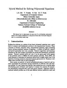
Figure 2: Distribution of real roots in [−10, 10] using kernel voting for 500 noiseless point matches, 200 estimations and λtrue = −0.2. (Left) Parasitic roots (green) vs. roots for mismatches (blue). (Center) Genuine roots. (Right) All roots, 100% of inliers. 0.4
0.3
3
0.2
0.3
2
0.1 0.2 0 0.1 0 −10
1
−0.1 −5
0
5
10
−0.2 −10
−5
0
5
10
0 −1
−0.5
0
0.5
1
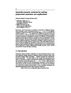
Figure 3: Distribution of real roots using kernel voting for 500 noiseless point matches, 100% inliers, 200 groups and λtrue = −0.2. (Left) Distribution of all roots in [−10, 10]. (Center) Distribution of all roots minus the distribution of roots from mismatches in [−10, 10]. (Right) Distribution of all roots in [−1, 1].
for f1 , f2 , f3 , f4 , f5 , f6 , f7 , f8 , f9 , λ. In this way we obtain 16 (complex) solutions. Generally less than 10 solutions are real.
4
Experiments
We test our algorithm on both synthetic (with various levels of noise, outliers and radial distortions) and real images and compare it to the existing 9-point algorithms for correcting radial distortion [6, 14]. We can get up to 16 complex roots. In general, more than one and less than 10 roots are real. If there is more than one real root, we need to select the best root, the root which is consistent with most measurements. To do so, we treat the real roots of the 16 (in general complex) roots obtained by solving the equations for one input as real roots from different inputs and use RANSAC [5, 10] or kernel voting [14] for several (many) inputs to select the best root among all generated roots. The kernel voting is done by a Gaussian kernel with fixed variance and the estimate of λ is found as the position of the largest peak. See [14] for more on kernel voting for this problem. To evaluate the performance of our algorithm, we distinguish three sets of roots. “All roots” is the set of all real roots obtained by solving the equations for K (different) inputs. “Genuine roots” denote the subset of all roots obtained by selecting the real root closest to the true λ for each input containing only correct matches. The set of genuine roots can be identified only in simulated experiments. “Parasitic roots” is the subset of all roots obtained by removing the genuine roots from all roots when everything is evaluated on inputs containing only correct matches. The results of our experiments for the kernel voting are shown in Figure 2. Figure 2 (Left) shows that the distribution of all real roots for mismatches is similar to the distribution of the parasitic roots. This allows to treat parasitic roots in the same way as the roots for mismatches. Figures 2 (Left and Center) show that the distribution of genuine roots is very sharp compared to the distribution of parasitic roots and roots for mismatches. Therefore, it is
Zuzana K´ukelov´a and Tom´asˇ Pajdla
2
0 −1
−0.5
0
0.5
1
2
3
1.5
2
1
1
0.5
0 −1
−0.5
0
0.5
1
0 −1
λtrue = −0.5
−0.5
0
0.5
1
λtrue = −0.5
0
0
−0.2
−0.2
computed λ
4
4
computed λ
6
[←]
−0.4
−0.6
−0.8
possible to estimate the true λ as the position of the largest peak, Figure 2 (Right). These experiments show that it is suitable to use kernel voting and that it make sense to select the best root by casting votes from all computed roots. It is clear from results shown in Figure 3 that it is meaningful to vote for λ’s either (i) within the range where the most of the computed roots fall (in our case [-10,10]), Figure 3 (Left), or (ii) within the smallest range in which we are sure that the ground truth lie (in our case [-1,1]), Figure 3 (Right). For large number of input data, it might also makes sense to subtract the apriory computed distribution of all real roots for mismatches from the distribution of all roots. 4.1
Tests on synthetic images
We initially studied our algorithm using synthetic datasets. Our testing procedure was as follows: 1. Generate a 3D scene consisting of N (= 500) random points distributed uniformly within a cuboid. Project M % of the points on image planes of the two displaced cameras. These are matches. In both image planes, generate (100 − M )% random points distributed uniformly in the image. These are mismatches. Altogether, they become undistorted correspondences. 2. Apply the radial distortion to the undistorted correspondences to generate noiseless distorted points. 3. Add Gaussian noise of standard deviation σ to the distorted points. 4. Repeat K times (We use K = 100 here, but in many cases K from 30 to 50 is sufficient). (a) Randomly choose 8 point correspondences from given N correspondences. (b) Normalize image point coordinates to [−1, 1] (c) Find up to 16 roots of the minimal solution to the autocalibration of radial distortion. (d) Select the real roots in the feasible interval, e.g., −1 < λ < 1 and the corresponding F’s. 5. Use kernel voting to select the best root. The resulting density functions for different outlier contaminations and for the noise level 1 pixel are shown in Figure 4. Here, K = 100, image size was 768 × 576 and λtrue = −0.25. In all cases, a good estimate, very close to the true λ, was found as the position of the maximum of
−0.6
−0.8
0
0.1 0.2 0.3 0.4 0.5 0.6 0.7 0.8 0.9
σ
−1
1
0
λtrue = −0.5 0
0
−0.2
−0.2
−0.4
−0.6
−0.8
−1
0.1 0.2 0.3 0.4 0.5 0.6 0.7 0.8 0.9
σ
1
λtrue = −0.5
computed λ
computed λ
Figure 4: Kernel voting results, for λtrue = −0.25, noise level σ = 0.2 (1 pixel), image size 768 × 576 and (Left) 100% inliers, (Center) 90% inliers (Right) 80% inliers. Estimated radial distortion parameters were (Left) λ = −0.2510 (Center) λ = −0.2546 (Right) λ = −0.2495.
−1
−0.4
−0.4
−0.6
−0.8
0
0.1 0.2 0.3 0.4 0.5 0.6 0.7 0.8 0.9
σ
1
−1
0
0.1 0.2 0.3 0.4 0.5 0.6 0.7 0.8 0.9
σ
1
Figure 5: Estimated λ as a function of noise σ, ground truth λtrue = −0.5 and (Top) inliers = 90%, (Bottom) inliers = 80%. Blue boxes contain values from 25% to 75% quantile. (Left) 8-point algorithm. (Right) 9-point algorithm.
the root density function. We conclude, that the method is robust to mismatches and noise. In the next experiment we study the robustness of our algorithm to increasing levels of Gaussian noise added to the distorted points. We compare our results to the results of two existing 9-point algorithms [6, 14]. The ground truth radial distortion λtrue was −0.5 and the level of noise varied from σ = 0 to σ = 1, i.e. from 0 to 5 pixels. Noise level 5 pixels is relatively large but we get good results even for this noise level and 20% of outliers. Figure 5 (Left) shows λ computed by our 8-point algorithm as a function of noise level σ. Fifty lambdas were estimated from fifty 8-tuples of correspondences randomly drawn for each noise level and (Top) 90% and (Bottom) 80% of inliers. The results are presented by the Matlab function boxplot which shows values 25% to 75% quantile as a blue box with red horizontal line at median. The red crosses show data beyond 1.5 times the interquartile range. The results for 9-point algorithms [6, 14], which gave exactly identical results, are shown for the same input, Figure 5 (Right). The median values (from -0.50 to -0.523) for 8-point as well as 9-point algorithms are very close to the ground truth value λtrue = −0.5 for all noise levels. The variances of the 9-point algorithms, Figure 5 (Right), are considerably larger, especially for higher noise levels, than the variances of the 8-point algorithm Figure 5 (Left). The 8-point algorithm thus produces higher number of good estimates for the fixed number of samples. This is good both for RANSAC as well as for kernel voting. 4.2
Tests on real images
The input images with relatively large distortion, Figures 1 (Left) and 6 (Left), were obtained as cutouts from 180◦ angle of view fish-eye images. Tentative point correspondences were found by the wide base-line matching algorithm [16]. They contained correct as well as incorrect matches. Distortion parameter λ was estimated by our 8-point algorithm and the kernel voting method. The input (Left) and corrected (Right) images are presented in Fig-
7
Solving polynomial equations for minimal problems in computer vision
Figure 6: Real data. (Left) Input image with significant radial distortion. (Right) Corrected image. 0.5 0.45 0.4 0.35 0.3 0.25 0.2 0.15 0.1 0.05 0 −10
−5
0
5
10
Figure 7: Distribution of real roots obtained by kernel voting for image in Figure 6. Estimated λ = −0.22.
ures 1 and 6. Figure 7 shows the distribution of real roots, for image from figure 6 (Left), from which λ = −0.22 was estimated as the argument of the maximum.
5
Conclusion
In this work we suggest improvements of current techniques for solving systems of polynomial equations and apply them to the minimal problem for the autocalibration of radial distortion. Our algorithm reduces the number of samples in RANSAC and is more stable than previously known 9-point algorithms. Our current MATLAB implementation of this algorithm runs about 0.05s on a P4/2.8GHz CPU. Most of this time is spent in the Gauss-Jordan elimination. However this time can be still reduced by further optimization. For comparison our MATLAB implementation of Fitzgibbon’s algorithm runs about 0.004s and the original implementation of Hongdong Li’s algorithm [14] based on MATLAB Symbolic-Math Toolbox runs about 0.86s.
Acknowledgement This work was supported by MSM6840770038 and the EC project FP6-IST-027787 DIRAC. Any opinions expressed in this paper do not necessarily reflect the views of the European Community. The Community is not liable for any use that may be made of the information contained herein.
References [1] C. Br¨auer-Burchardt and K. Voss. A new algorithm to correct fish-eye and strong wide-angle-lens-distortion from single images. ICIP 2001, pp. 225–228. [2] D. Cox, J. Little, and D. O’Shea. Using Algebraic Geometry. Springer-Verlag, 2005. [3] D. Cox, J. Little, and D. O’Shea. Ideals, Varieties, and Algorithms. Springer-Verlag, 1992.
8
[←]
[4] D. Devernay and O. Faugeras. Straight lines have to be straight. MVA, 13(1):14–24, 2001. [5] M. A. Fischler and R. C. Bolles. Random Sample Consensus: A paradigm for model fitting with applications to image analysis and automated cartography. Comm. ACM, 24(6):381–395, 1981. [6] A. Fitzgibbon. Simultaneous linear estimation of multiple view geometry and lens distortion. CVPR 2001, pp. 125–132. [7] J.-C. Faugere. A new efficient algorithm for computing gr¨obner bases (f4 ). Journal of Pure and Applied Algebra, 139(1-3):61–88, 1999. [8] X.-S. Gao, X.-R. Hou, J. Tang, and H.-F. Cheng. Complete solution classification for the perspective-three-point problem. IEEE PAMI, 25(8):930–943, 2003. [9] R. Hartley and S. Kang. Parameter-free radial distortion correction with centre of distortion estimation. ICCV 2005, pp. 1834–1841. [10] R. Hartley and A. Zisserman. Multiple View Geometry in Computer Vision. Cambridge University Press, 2003. [11] S. Kang. Catadioptric self-calibration. CVPR 2000, [12] S. Kang. Radial distortion snakes. IAPR MVA Workshop 2000, pp. 603–606, Tokyo. [13] H. Li. A simple solution to the six-point two-view focal-length problem. ECCV 2006, pp. 200–213. [14] H. Li and R. Hartley. A non-iterative method for correcting lens distortion from nine-point correspondences. OMNIVIS 2005. [15] H. Li and R. Hartley. Five-point motion estimation made easy. ICPR 2006, pp. 630–633. [16] J. Matas, O. Chum, M. Urban, and T. Pajdla. Robust wide-baseline stereo from maximally stable extremal regions. Image and Vision Computing, 22(10):761–767, 2004. [17] B. Micusik and T. Pajdla. Estimation of omnidirectional camera model from epipolar geometry. CVPR 2003, [18] D. Nister. An efficient solution to the five-point relative pose. IEEE PAMI, 26(6):756–770, 2004. [19] R. Steele and C. Jaynes. Overconstrained linear estimation of radial distortion and multi-view geometry. ECCV 2006, [20] G. Stein. Lens distortion calibration using point correspondences. CVPR 1997, pp. 600:602. [21] H. Stewenius. Gr¨obner basis methods for minimal problems in computer vision. PhD thesis, Lund University, 2005. [22] H. Stewenius, C. Engels, and D. Nister. Recent developments on direct relative orientation. ISPRS J. of Photogrammetry and Remote Sensing, 60:284–294, 2006. [23] H. Stewenius, D. Nister, F. Kahl, and F. Schaffalitzky. A minimal solution for relative pose with unknown focal length. In CVPR 2005, pp. 789–794. [24] H. Stewenius, D. Nister, M. Oskarsson, and K. Astrom. Solutions to minimal generalized relative pose problems. OMNIVIS 2005. [25] R. Strand and E. Hayman. Correcting radial distortion by circle fitting. BMVC 2005. [26] S. Thirthala and M. Pollefeys. Multi-view geometry of 1d radial cameras and its application to omnidirectional camera calibration. ICCV 2005, pp. 1539–1546. [27] S. Thirthala and M. Pollefeys. The radial trifocal tensor: A tool for calibrating the radial distortion of wide-angle cameras. CVPR 2005 pp. 321–328. [28] R. Tsai. A versatile camera calibration technique for high-accuracy 3d machine vision metrology using off-the-shelf tv cameras and lenses. IEEE J. of Robotics and Automation, 3(4):323344, 1987. [29] Z. Zhang. On the epipolar geometry between two images with lens distortion. In ICPR 1996. [30] Z. Zhang. A flexible new technique for camera calibration. IEEE PAMI, 22(11):1330–1334, 2000.