solving practical vehicle routing problem with time windows using ...

F. Taner, A. Galić, T. Carić: Solving Practical Vehicle Routing Problem with Time Windows Using Metaheuristic Algorithms

FILIP TANER, B.Eng. E-mail: [email protected] ANTE GALIĆ, B.Eng. E-mail: [email protected] TONČI CARIĆ, Ph.D. E-mail: [email protected] University of Zagreb, Faculty of Transport and Traffic Sciences Vukelićeva 4, 10000, Zagreb, Croatia

Distribution Logistics Review Accepted: July 13, 2011 Approved: July 5, 2012

SOLVING PRACTICAL VEHICLE ROUTING PROBLEM WITH TIME WINDOWS USING METAHEURISTIC ALGORITHMS

ABSTRACT This paper addresses the Vehicle Routing Problem with Time Windows (VRPTW) and shows that implementing algorithms for solving various instances of VRPs can significantly reduce transportation costs that occur during the delivery process. Two metaheuristic algorithms were developed for solving VRPTW: Simulated Annealing and Iterated Local Search. Both algorithms generate initial feasible solution using constructive heuristics and use operators and various strategies for an iterative improvement. The algorithms were tested on Solomon’s benchmark problems and real world vehicle routing problems with time windows. In total, 44 real world problems were optimized in the case study using described algorithms. Obtained results showed that the same distribution task can be accomplished with savings up to 40% in the total travelled distance and that manually constructed routes are very ineffective.

KEY WORDS vehicle routing problem with time windows, simulated annealing, iterated local search, metaheuristcs

1. INTRODUCTION Vehicle routing problem (VRP) is interesting to the scientific community because of the possibility of greatly reducing transportation costs by successfully solving the problem. Optimization of delivery routes is important because transport costs influence the overall cost of the delivered goods. In this field of combinatorial optimization many scientific papers and surveys were published [1, 2, 3, 4, 5]. Algorithms for VRP optimization can help to solve many different logistics problems in distribution. Manually constructed routes are very inefficient and can be significantly improved by algorithms for solving VRP. This is done by

reducing overall travelled distance, number of vehicles used and total waiting time. When planning delivery routes for their products, logistic companies are facing a problem that can be classified as one of the VRP instances, depending on the given constraints. Most common constraints are time windows and limited capacities of vehicles which define Vehicle Routing Problem with Time Windows (VRPTW). In solving VRPTW exact methods evaluate every possible solution, but those methods are extremely time-consuming, even when using high-end computers. Metaheuristic methods can produce reasonably good solutions in relatively short time. Two metaheuristic strategies for solving VPRTW were applied: Simulated Annealing and Iterative Local Search. Algorithm parameters were tuned to specific set of problems. Both strategies were tested on Solomon’s benchmark problems, as well as on 44 real world problems as case study.

2. VEHICLE ROUTING PROBLEM Vehicle routing problem is NP-hard problem defined by the task of determining the optimal set of routes to be performed by a fleet of vehicles to serve a given set of customers [6]. The solution of the VRP is a set of routes which all begin and end in the depot and where all customers are served only once [4]. The VRP is combinatorial optimization problem on the graph. Let G = ^V, Ah is fully connected graph with a set of vertices V = "0, f, n, . Vertex with index 0 is depot, while other vertices have indices i = 1, 2, f, n and represent customers. Every arc î, jh from the set of arcs A has non-negative transportation cost cij which can represent the cost of fuel or distance between customers or some other combination of costs. In a case when one way streets exists in a street topology, the asymmetric

Promet – Traffic&Transportation, Vol. 24, 2012, No. 4, 343-351

343

F. Taner, A. Galić, T. Carić: Solving Practical Vehicle Routing Problemwith Time Windows Using Metaheuristic Algorithms

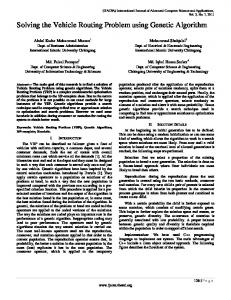
graphs are used where costs in opposite direction are not same cij ! c ji . The homogeneous fleet of K vehicles is available in the depot and each vehicle is used only for one route which begins and ends in the depot. Let route of single vehicle R is sequence of customers starting and ending in the depot. If there are only capacity constrains in the problem it can be treated as Capacitated Vehicle Routing problem (CVRP). Each customer has non-negative demand mi while each vehicle ki is limited by maximal capacity qi . Basic variant of problem can be extended by additional constraints. Figure 1 shows different variants of VRP problem and relations between them [1].

VRP Capacity constraints

g ulin

a ckh

Ba

VRPB

CVRP Time Windows

Mix ed ser vic e

VRPTW

VRPBTW

VRPPD

VRPPDTW

Figure 1 - VRP variants and their interconnections Source: prepared by the author on the basis of [1]

If customers request delivery within a specific time window, the problem can be modelled as vehicle routing problem with time windows (VRPTW). In case of simultaneous pickup and delivery of goods, the problem can be modelled as vehicle routing problem with pickup and delivery (VRPPD). In case of vehicle routing problem with backhauls (VRPB), a vehicle needs to collect goods after it completes delivery. Last two problems can also be extended with time constraints (VRPBTW and VRPPDTW). In this paper the practical problem of postal delivery company is modelled as the VRPTW problem. Service of each customer has to be done inside time window 6ei, li @ , where ei is earliest and li latest possible time when service must occur. If vehicle arrives before opening of time window it has to wait. It is forbidden to start service after closing of time window li because it would produce an unfeasible solution. The depot has also time window that represent its opening and closing time. The primary objective of VRPTW optimization is to find the minimal number of vehicles that can accomplish delivery task in a way that each route satisfies all time and capacity constraints and that each customer is serviced only once. The secondary objective is to minimize overall travelled distance or time. 344

3. INITIAL SOLUTION In order to effectively solve VRPTW problem, it is necessary to obtain a feasible initial solution in which all constraints are satisfied. Due to the fact that finding of a feasible solution for VRPTW problem with minimal number of vehicles is a very complex task, constructive heuristic algorithms often produce solutions of bad quality which serve only as a starting point for further optimization. Best known constructive algorithm for VRPTW is Solomon I1 heuristic. Simplified description is presented in Algorithm 1 and more details can be found in original paper [7]. Function FindSeed() selects the first customer which will be inserted into the vehicle route. Criteria for its selection are the measure of how far away it is from the depot and how close is its time window opening. Inside main loop function FindNewCustomer(v) searches for un-served customer that can be inserted into a route of current vehicle v without violation of time and capacity constraints. If it fails, a new vehicle is engaged and a new seed customer is added to the route. Function Terminate() checks if there are more un-routed customers. Algorithm 1. Solomon’s I1 insertation heuristic

procedure SolomonI1() c := FindSeed() v :=NewVehicle() AddToRoute(c, v) while not Terminate() do c := FindNewCustomer(v) if c != null then InsertCustomer(c, v) else c:=FindSeed() v :=NewVehicle() AddToRoute(c, v) endif endwhile return CurrentSolution() end

4. IMPROVEMENT OPERATORS Initial solution can be significantly improved by simple operations such as relocation, exchange and reposition of customers in/between routes of vehicles. Simplest improvement operators are presented bellow and more complex ones can be found in [8]. Intra Route operators relocate one or more customers from one position in route to another position in same route. Inter Route operators relocate and exchange customers between two different routes. Intra Relocate operator shown in Figure 2 removes one customer from a route and inserts it to the other position inside the same route. Such operation will cause shifting of one Promet – Traffic&Transportation, Vol. 24, 2012, No. 4, 343-351


R

a0

a2

R'

a0

a2

a1

b1

a1

b0

b1

b0

Figure 2 - Intra Relocate operator Source: prepared by the author on the basis of [13]

R

a0

b0

b1

a1

R'

a0

b0

b1

a1

Figure 3 - Intra TwoOpt operator Source: prepared by the author on the basis of [13] a0

a2

a0

R1

a1

R2

a2

R1'

b0

a1

R2'

b1

b0

b1

Figure 4 - Inter Relocate operator Source: prepared by the author on the basis of [13]

or more customers as well. The customer a1 is inserted between customers b0 and b1 if there is a positive saving in the new route Rl . Saving u is expressed as the following sum: u = ^câ0, a1h + câ1, a2h + c^b0, b1hh -^câ0, a2h + c^b0, a1h + câ1, b1hh (1) Intra TwoOpt operator shown in Figure 3 modifies route in such a way that it removes crossings in the route R and reverses travel directions between customers b0 and a1 . Savings u produced by a new route Rl have to be positive and they are expressed as the following sum: (2) u = ^câ0, a1h + c^b0, b1hh - ^câ0, b0h + câ1, b1hh Beside savings calculation in Intra Route operators it is also necessary to check for feasibility of the time window constraints for new route Rl . Capacity constraints do not need to be checked because they are already examined in route R. Inter Relocate operator shown in Figure 4 removes customer a1 from route R1

and inserts it between customers b0 and b1 in new route R2l if there is positive saving expressed as the following sum: u = ^câ0, a1h + câ1, a2h + c^b0, b1hh -^câ0, a2h + c^b0, a1h + câ1, b1hh

(3)

Route R1l will keep all constraints fulfilled after removal of a1 but for route R2l time and capacity feasibility has to be checked because insertion of a1 can produce overload and delay to customers. Inter Exchange operator shown in Figure 5 swaps two customers from different routes. Customer a1 from route R1 is exchanged with customer b1 from route R2 . It is necessary to check the feasibility of both routes and reject exchange combination " a1, b1 , if it will produce overload or delay in any of two routes. Savings of exchange move are expressed as the following sum: u = ^câ0, a1h + câ1, a2h + c^b0, b1h + c^b1, b2hh -^câ0, b1h + c^b1, a2h + c^b0, a1h + câ1, b2hh

Promet – Traffic&Transportation, Vol. 24, 2012, No. 4, 343-351

(4) 345


a0

V1

a2

V 1'

b1

a1

V2 b2

a0

a1

V 2' b0

a2 b1

b2

b0

Figure 5 - Inter Exchange operator Source: prepared by the author on the basis of [13]

It is important to note that each improvement operator among all feasible moves selects the one that will produce maximal saving u.

5. LOCAL SEARCH AND METAHEURISTICS Improvement operators are iteratively applied in the local search procedure in order to improve solution as much as possible. Each operator searches for narrow neighbourhood of the current solution and tries to find a better one. Eventually, local search will stop in a local optimum or suboptimal solution if there are no feasible solutions that can be found using the same improvement operators. In order to continue improving the obtained solution it is necessary to move to another area of solution space by temporarily accepting worse solutions and applying the local search again. Metaheuristic methods are developed in order to reduce the solution search space and to consider evaluating only areas which have high probability to contain good solutions. Moving from one neighbourhood to another by accepting worse solutions can lead to global optima in successive iterations of local search.

5.1 Simulated annealing Methodology of SA is analogous to the physical process of annealing in metallurgy [9, 10, 11]. In order to obtain perfect crystal structures of metal without irregularities, solid metals are melted and then cooled down slowly. Heat enables atoms to become unstuck from their initial positions which correspond to local optimum of minimal energy and wander randomly through states of higher energy. In this analogy, the different energy levels represent candidate solutions, and evaluation function represents the internal energy of the solid [12]. Cooling needs to be done slowly in order to increase the chance of getting a configuration with minimal internal energy (global optimum). Simulated annealing (Algorithm 2) starts from the initial feasible solution obtained by Solomon’s I1 insertion heuristic described in the previous section (Algorithm 1). In each iteration of the main loop function Escape(s) 346

generates new solution sl using modified variants of Intra Relocate, Inter Relocate and Inter Exchange operators in which negative savings are allowed. In the next step local search procedure is applied in order to produce solution sm which represents local optimum [13]. Solution sm is automatically accepted as starting point for next iteration if objective function yields better value than for solution s. Otherwise, acceptance criterion for solution sm follows the probability function known as Metropolis condition [11]: pt = e-

f^ smh - f^ sh T

(5)

Temperature T determines how likely solution sm will be accepted. As temperature drops throughout the process, the probability of accepting worse solution decreases. This is called cooling schedule and determines the number of iterations of the algorithm. The cooling schedule is a geometric function T = T $ a , where 0 # a 1 1 . The maximal (initial) and the minimal temperature are empirically determined for each problem set. The objective function that evaluates the quality of the given solution is calculated as follows: (6) f ^ s h = v s $ ds where vs is the number of vehicles used in the solution and ds is the sum of route distances. Solution best is updated in case of improvement of the evaluation function (6). The first factor of this function greatly increases the value of the function thus forcing the algorithm to accept solutions with less used vehicles (routes). The second factor is needed to reduce the overall distance if the number of the used vehicles is maintained. Function Terminate() is responsible for stopping the algorithm after temperature T reaches its allowed minimum. Additionally, the temperature is reset to the initial value a given number of times, to repeat the cooling process again starting from the best solution found at the time. Algorithm 2. Simulated Annealing

procedure SA() T := InitialTemperature() init := SolomonI1() s := LocalSearch(init) Promet – Traffic&Transportation, Vol. 24, 2012, No. 4, 343-351


best := s while not Terminate() do s’ := Escape(s) s” := LocalSearch(s’) if (f (s’’)