Solving the Vehicle Routing Problem by Using Cellular Genetic Algorithms Enrique Alba1 and Bernab´e Dorronsoro2 1
Department of Computer Science, University of M´ alaga
[email protected] Central Computer Services, University of M´ alaga
[email protected]
2
Abstract. Cellular Genetic Algorithms (cGAs) are a subclass of Genetic Algorithms (GAs) in which the population diversity and exploration are enhanced thanks to the existence of small overlapped neighborhoods. Such a kind of structured algorithms is specially well suited for complex problems. In this paper we propose the utilization of some cGAs with and without including local search techniques for solving the vehicle routing problem (VRP). A study on the behavior of these algorithms has been performed in terms of the quality of the solutions found, execution time, and number of function evaluations (effort). We have selected the benchmark of Christofides, Mingozzi and Toth for testing the proposed cGAs, and compare them with some other heuristics in the literature. Our conclusions are that cGAs with an added local search operator are able of always locating the optimum of the problem at low times and reasonable effort for the tested instances.
1
Introduction
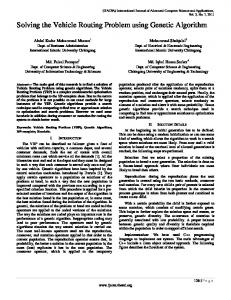
Transportation is a major problem domain in logistics, and so it represents a substantial task in the activities of many companies. In some market sectors, transportation means a high percentage of the value added to goods. Therefore, the utilization of computerized methods for transportation often results in significant savings ranging from 5% to 20% in the total costs, as reported in [1]. A distinguished problem in the field of transportation consists in defining the optimal routes for a fleet of vehicles to serve a set of clients. In this problem an arbitrary set of clients must receive goods from a central depot. This general scenario presents many chances for several concrete definitions of subclasses of problems: determining the optimal number of vehicles, finding the shortest routes, etc. all this subject to many restrictions like vehicle capacity, time windows for deliveries, etc. This variety of scenarios leads to a plethora of problem variants in practice. The basic problem class we address in this paper is known as the Vehicle Routing Problem (VRP) [2], which consists in delivering goods to a set of customers with known demands through minimum-cost vehicle routes originating and terminating at the depot, as seen in Fig. 1 –for a more detailed description of the problem see Sect. 2. The VRP is an important class of problem, since solving it is equivalent to solving multiple TSP problems at once, and thus it has been studied both theo-
2
Depot
VRP
a)
Depot
b)
Fig. 1. The Vehicle Routing Problem finds the minimum cost routes –b)– to serve a set of customers (points) geographically distributed, from a depot –a)–
retically and in practice [3]. There is a large number of extensions to the canonical VRP, but in this paper, we address the base problem without time windows. There has been a steady evolution in the design of solution methodologies in the past, both exact and approximate, for this problem. However, no known exact method is capable of consistently solving to optimality instances involving more than 50 customers [1]. Instead, heuristics are mostly preferred. The contribution of this work is to define a powerful yet simple Cellular Genetic Algorithm (cGA) [4] that is able to compete with the best known approaches in the resolution of the VRP in terms of the solution found, the execution time, and the number of evaluations made. In addition, it represents a kind of paradigm much simpler of customization and comprehension than others such as Tabu Search (TS) or very specialized hybrid algorithms. Local search techniques can be quite naturally embedded into a cGA, and we test here to which extent it can be advantageous. We test our algorithms over a selection of the Christofides et al. [3] benchmark instances, and compare our results with some other known heuristics. The paper is arranged in the following manner. Section 2 gives a mathematical formulation for the VRP. Our cGA is described in Sect. 3. Section 4 presents the results of our algorithms, and compares them with those of some heuristics in the literature. The conclusions and some future work lines are presented in Sect. 5.
2
Vehicle Routing Problem (VRP)
The VRP is a well known integer programming problem which falls into the category of NP-hard problems [5]. It is defined on an undirected graph G = (V , E) where V = {v0 , v1 , . . . , vn } is a vertex set and E = {(vi , vj )/vi , vj ∈ V , i < j} is an edge set. The depot is represented by vertex v0 , and it is from where that m identical vehicles of capacity Q must service all the cities or customers, represented by the set of n vertices {v1 , . . . , vn }. We define on E a non-negative cost, distance or travel time matrix C = (cij ) between customers vi and vj . Each customer vi has non-negative demand qi and drop time δi (time needed to unload all
3
goods). Let be R1 , . . . , Rm a partition of V representing the routes of the vehicles to service all the customers. The cost of a given route (Ri ={v0 , v1 , . . . , vk+1 }), where vj ∈ V and v0 = vk+1 = 0 (0 denotes the depot), is given by: Cost(Ri ) =
k X
cj,j+1 +
k X
δj ,
(1)
j=0
j=0
and the cost of the problem solution (S) is: FVRP (S) =
m X
Cost(Ri ) .
(2)
i=1
The VRP consists in determining a set of a maximum of m routes (i) of minimum total cost (see (2)); (ii) starting and ending at the depot v0 ; and such that (iii) each customer is visited exactly once Pby exactly one vehicle; (iv) the total demand of any route does not exceed Q ( vj ∈Ri qj ≤ Q); and (v) the total duration of any route is not larger than a preset bound D (Cost(Ri ) ≤ D). The number of vehicles is either an input value or a decision variable. In this study, the length of routes is minimized independently of the used number of vehicles.
3
Algorithms for Solving the VRP
In this section we discuss the algorithms we plan to use later in the paper to solve the VRP. Initially we present a cGA with structured population as the basic tool for the search. In addition, since there exists a long tradition in VRP to include local search techniques to improve partial solutions; and, since in cGAs it is quite direct to include such kind of procedures, we will further discuss in this section several mechanisms to perform local optimization: 2-Opt and λ-Interchange. 3.1
Cellular Genetic Algorithms for the VRP
Genetic Algorithms (GAs) are based on an analogy with biological evolution. A population of individuals representing tentative solutions is maintained. New individuals are produced by combining members of the population, and these replace existing individuals with some policy. Cellular GAs are a subclass of GAs in which the population is structured in a specified topology, so that individuals may only interact with their neighbors (see Fig. 2). These overlapped small neighborhoods help in exploring the search space because the induced slow diffusion of solutions through the population provides a kind of exploration, while exploitation takes place inside each neighborhood by genetic operations. In Algorithm 1 we can see a pseudocode of our basic cGA [6]. In this cGA, the population is structured in a 2D toroidal grid, and the neighborhood defined on it –line 5– always contains 5 individuals: the considered one (position(x,y)) plus the North, East, West, and South individuals (called NEWS, linear5, or Von Neumann). Binary tournament selection is used in the
4
Algorithm 1 Pseudocode of cGA 1: proc Steps Up(cga) //Algorithm parameters in ‘cga’ 2: for s ← 1 to MAX STEPS do 3: for x ← 1 to WIDTH do 4: for y ← 1 to HEIGHT do 5: n list←Get Neighborhood(cga,position(x,y)); 6: parents←Local Select(n list); 7: aux indiv←Recombination(cga.Pc,parents); 8: aux indiv←Mutation(cga.Pm,aux indiv); 9: aux indiv←Local Search(cga.Pl,aux indiv); 10: Evaluate Fitness(aux indiv); 11: Insert If Better(position(x,y),aux indiv,cga,aux pop); 12: end for 13: end for 14: cga.pop←aux pop; 15: Update Statistics(cga); 16: end for 17: end proc Steps Up;
Panmictic GA
Cellular GA
Fig. 2. Panmictic and cellular populations
neighborhood for the first parent, while the other one is the considered individual itself (Local Select) (line 6). Genetic operators are applied to the individuals in lines 7 and 8 (explained in Sect. 3.1). We can add different local search techniques to our basic cGA by simply including line 9 to the algorithm (see Sect. 3.2). After applying these operators, we evaluate the fitness value of the new individual (line 10), and insert it on its equivalent place in the new population –line 11– only if its fitness value is larger than the parent’s one (elitist replacement). After applying the above mentioned operators to the individuals we replace the old population by the new one (line 14), and we calculate some statistics (line 15). It can be seen how in our algorithm new individuals replace old ones en bloc (synchronously) and not incrementally. The fitness value assigned to every individual is computed like follows: f (S) = FVRP (S) + λ · overcap(S) + µ · overtm(S) ,
(3)
feval (S) = fmax − f (S) .
(4)
The objective of our algorithm is to maximize feval (S) (4) by minimizing f (S) (3). The value fmax must be larger or equal to that of the worst feasible solution for the problem. Function f (S) is calculated by adding the total costs of all the routes (FVRP (S)), and penalizes the fitness value if the capacity of any vehicle and/or the time of any route are exceeded. Functions overcap(S) and overtm(S) return the overhead in capacity and time, respectively, of the solution with respect to the maximum allowed value of each route. These values returned by overcap(S) and overtm(S) are weighted by multiplying them with the values λ and µ, respectively. Representation of Individuals. In a GA, individuals represent candidate solutions. A candidate solution to an instance of the VRP must specify the number of vehicles required, the allocation of the demands to all these vehicles, and also
5
the delivery order of each route. We adopted a representation consisting of a permutation of integers. Each permutation will contain both customers and route splitters (delimiting different routes), so we will use a permutation of numbers [0 . . . n − 1] with length n = c + k for representing a solution for the VRP with c customers and a maximum of k + 1 possible routes. Customers are represented with numbers [0 . . . c − 1], while route splitters belong to the range [c . . . n − 1].
{
{
{
{
4 - 5 - 2 - 10 - 0 - 3 - 1 - 12 - 7 - 8 - 9 - 11 - 6 Route 1
Route 2
Route 3
Route 4
Fig. 3. Individual representing a solution
Each route is composed by the customers in the individual between two route splitters. For example, in Fig. 3 we plot an individual representing a possible solution for a VRP instance with 10 customers using 4 vehicles at most. Values [0, . . . , 9] represent the customers while [10, . . . , 12] are the route splitters. Route 1 begins at the depot, visits customers 4–5–2 (in that order), and returns to the depot. Route 2 goes from the depot to customers 0–3–1 and returns. The vehicle of Route 3 starts at the depot and visits customers 7–8–9. Finally, in Route 4, only customer 6 is visited. This representation allows empty routes by simply placing two route splitters together without clients between them. Genetic Operators. Two genetic operators are applied to all the individuals with preset probabilities along the evolution. These two operators are recombination and mutation. The recombination operator we use is an edge recombination operator (ERX ) [7], that builds an offspring by preserving edges from both parents. The mutation operator used in the algorithm consists in applying Insertion, Swap or Inversion operations to each gene with equal probability (see Fig. 4). The Insertion [8] operator selects a customer and inserts it in another randomly selected place. Swap [9] consists in randomly selecting two customers and exchanging them. Finally, Inversion [10] reverses the visiting order of the customers between two randomly selected cut points. In all the three operators changes might occur in an intra or inter-route way. Insertion 12345678
Swap 12345678
Inversion 12345678
Offspring 1 2 3 5 6 7 4 8
12543678
12654378
Parent
Fig. 4. The three different mutations used
6
3.2
Local Search
It is very clear after all the existing literature on VRP that local search is almost mandatory to achieve results of high quality [11] [12]. This is why we envision from the beginning the application of two of the most successful techniques in the past years. Then we will not only consider canonical cGAs for VRP, but also will add a local post-optimization step by applying 2-Opt [13] and/or λ-Interchange [14] local optimization methods to every individual after each generation. The 2-Opt simple local search method works inside each route. It randomly selects two non-adjacent edges (i.e. (a, b) and (c, d)) of a single route, delete them, thus breaking the tour into two parts, and then reconnects those parts in the other possible way (i.e. (a, c) and (b, d)). The λ-Interchange local optimization method we use is based on the interchange of all the possible combinations for up to λ customers between sets of routes. Hence, this method results in customers either being shifted from one route to another, or being exchanged between routes. The mechanism can be described as follows. A solution to the problem is represented by a set of routes S = {R1 . . . Rp . . . Rq . . . Rk }, where Ri is the set of customers serviced in route i. New neighboring solutions can be obtained by applying λ-Interchange between a pair of routes Rp and Rq by replacing each subset of customers S1 ⊆ Rp of size |S1 | ≤ λ with any otherSone S2 ⊆ Rq of size |S2 |S ≤ λ. This way, we get two new routes Rp0 = (Rp − S1 ) S2 and Rq0 = (Rq − S2 ) S1 , which are part of the new solution S 0 = {R1 . . . Rp0 . . . Rq0 . . . Rk }.
4
Experimentation
In this section we describe the experiments applying these ideas to a set of problems taken from the well-known OR library [15]. Our algorithms have been implemented in Java on a 2.4 GHz PC (Linux OS). They have been tested with instances C1, C2, C3, C6, C7, C8, C12, and C14 [3] (not enough room for the whole benchmark). The first three instances contain data for 50, 75, and 100 customers respectively, with capacity restrictions on vehicles but not on the distance. Datasets C6, C7 and C8 are like C1, C2 and C3, respectively, with the additional restrictions of maximal route distance and the existence of a drop time. An additional feature of C12 with respect to the three first ones is that the 100 customers to visit are geographically clustered. The last instance included, C14 is really the C12 instance with the restrictions of maximal route distance and the addition of drop times. We have used four different algorithms, all of them extracted from the metaheuristic sheet of a cGA described in Sect. 3. The difference among them is just the local search method used. The first algorithm studied does not use any local search method (cGA). The second one uses the 2-Opt method (cGA2o). The two last studied algorithms use 2-Opt plus a λ-Interchange (with a maximum of 20 search steps), and return the best individual found with any of the two methods on each local search step. These algorithms differ in the value of λ used. One of them implements λ = 1 (cGA2o1i), and the other one utilizes λ = 2 (cGA2o2i).
7
For each individual, the recombination probability is set to 0.65 in all of our algorithms. The mutation probability for an individual is 0.85, and its alleles are mutated with probability 1/L, being L the length of the chromosome. The local search (if used) is applied to all individuals (probability 1.0). Population size is 100 individuals in any case, and we perform 30 independent runs to get reliable statistical results. For the evaluation of the fitness value, we have used values 107 , 103 and 103 for parameters fmax , λ and µ, respectively. Next, in Sect. 4.1, we present the results obtained with our proposed algorithms, while in Sect. 4.2 we compare our results with the existing literature. 4.1
Performance of the Proposed Algorithms
Let us now proceed to analyze the results. The proposed algorithms can easily be compared by consulting tables 1, 2 and 3, containing the best solution found (total route distance), and the average execution time and number of evaluations needed, respectively. The optimum values are bolded for the reader’s commodity. Our conclusions are quite stable and relatively clear. The results worked out by the canonical cGA (Table 1) are far from the best known results for the tested instances. However, just by including a local improvement with 2-Opt (cGA2o algorithm) the total cost of the solutions found in all the instances is greatly reduced with respect to cGA, although no optimal solution is still found. It is by adding the λ-Interchange local optimization that we achieve really interesting results, since we can solve all the instances to the optimum. Table 1 shows that cGA2o1i finds the best known solution for all the instances, having a similar behavior as for cGA2o2i (being this last only slightly less accurate for C3). If we analyze average execution times (see Table 2, figures in seconds), then we can appreciate a clear increment as the complexity of the algorithms is enlarging: this sounds common sense. Therefore, the simpler the algorithm the smaller the execution time. In most cases times are quite affordable and reasonable. Finally, Table 3 shows the average number of function evaluations made by the algorithm during the search. The effort for cGA and cGA2o is difficult to evaluate since it is an effort to lead the algorithm to a local optimum (most runs reach the maximum number of allowed evaluations without finding a solution). On the other hand, the numerical effort of cGA2o1i and cGA2o2i are quite similar and meaningful, indicating that cGA2o1i is preferable over cGA2o2i since it performs a search of similar accuracy in a smaller time. As a final conclusion, we can point out cGA2o1i as being the more accurate algorithm showing very reasonable times and effort to locate the optimum. The other algorithms are either too explorative (inaccurate) or unnecessarily complex. 4.2
Comparison Against Other Techniques
In this section we compare our algorithms against the best so far techniques reported in the literature, as any rigorous work should do. We have selected some classic algorithms, like savings [16], sweep [17], 1-petal or 2-petal [18], and
8 Table 1. Best solution found C1 C2 C3 C6 C7 C8 C12 C14
cGA 548.83 907.53 937.36 568.83 1030.23 1053.82 986.62 1007.92
cGA2o cGA2o1i cGA2o2i 533.09 524.61 524.61 874.41 835.26 835.26 838.70 826.14 827.39 558.99 555.43 555.43 973.48 909.68 909.68 903.66 865.94 865.94 891.32 819.56 819.56 904.43 866.37 866.37
Table 2. Average time (in seconds) C1 C2 C3 C6 C7 C8 C12 C14
cGA 3.53 ± 0.11 4.81 ± 0.11 7.86 ± 0.25 3.54 ± 0.08 4.80 ± 0.08 7.93 ± 0.31 7.40 ± 0.49 7.87 ± 0.24
cGA2o 11.28 ± 0.63 23.45 ± 0.71 60.47 ± 2.27 9.85 ± 0.31 20.02 ± 0.70 49.75 ± 2.10 53.21 ± 2.34 47.63 ± 2.01
cGA2o1i 42.38 ± 1.82 252.54 ± 16.26 516.74 ± 30.58 47.68 ± 2.24 268.11 ± 12.95 628.16 ± 191.95 485.58 ± 82.60 583.54 ± 65.22
cGA2o2i RT Prins BB 48.63 ± 1.98 11 < 1 120 289.06 ± 11.32 68 184 860 569.14 ± 29.76 900 497 1674 55.92 ± 6.92 — 106 140 312.08 ± 137.59 — 315 630 659.81 ± 28.02 — 664 303 536.42 ± 26.96 350 7 433 651.54 ± 32.26 — 591 284
Table 3. Average number of evaluations C1 C2 C3 C6 C7 C8 C12 C14
cGA 100100.0 ± 0.0 120100.0 ± 0.0 150100.0 ± 0.0 100100.0 ± 0.0 120100.0 ± 0.0 150100.0 ± 0.0 150100.0 ± 0.0 150100.0 ± 0.0
cGA2o 213310.10 ± 1770.36 373167.20 ± 4875.20 481971.10 ± 6458.94 211402.10 ± 1649.12 365590.50 ± 3716.58 475392.50 ± 6469.34 488714.20 ± 8261.53 486746.80 ± 7819.13
cGA2o1i 71725.73 ± 2257.59 171668.90 ± 7818.45 210094.10 ± 9350.17 75029.00 ± 2729.36 170737.40 ± 6055.16 227187.80 ± 9307.24 193967.70 ± 8113.52 222168.50 ± 7604.63
cGA2o2i 72370.60 ± 2741.85 170747.50 ± 5825.33 208350.70 ± 8665.93 75023.80 ± 2442.21 171175.10 ± 5889.34 223854.50 ± 9126.49 193482.90 ± 6525.01 221596.50 ± 9429.92
some newer ones like tabu search TS, other GAs, and also ant systems. These three last techniques are known to perform very well on the VRP. The TS algorithm included is that of Rochat and Taillard [11] (RT), the genetic algorithms are those of Prins [19], and Berger and Barkaoui [12] (BB), and, the two ant algorithms included are very recent works proposed by Bullnheimer et al. [20] (AS) and SavingsAnts, by Doerner et al. [21] (SA). As shown in Table 4, RT, Prins, and cGA2o1i outperform the other algorithms, finding the best known solution for all the studied instances. Hence, the two mentioned ant algorithms perform with a lower accuracy than existing TS and GAs. We must however point out a clear distinction: we are just hybridizing two canonical algorithms whose definitions are simple and extremely easy for customization on these and other similar problems. The same cannot be said for other highly specialized algorithms, that require a great customization effort from the researchers. Simplicity and clarity (and even potential extensibility) are a clear contribution of our algorithms with respect to the others. In Table 2 we compare all the algorithms for which execution times have been reported. Times of RT are calculated by the authors on a Silicon Graphics Indigo –100 MHz– (no run-times were provided for C6, C7, C8 and C14), the genetic
9
algorithm of Prins is implemented in Delphi on a 500 MHz PC under Windows 95, and BB is implemented in C++ on a 400 MHz Pentium processor. The algorithm of Prins is the globally faster for instances C1, C3 and C12, while RT is the fastest one just in the case of C2. The best times for instances C8 and C14 are hold by BB, and finally, our cGA2o1i is faster than the others for instances C6 and C7.
Table 4. Our best cGA vs. other heuristics and best known solutions C1 C2 C3 C6 C7 C8 C12 C14
5
Savings 578.56 888.04 878.70 616.66 974.79 968.73 824.42 868.50
Sweep 531.90 884.20 846.34 560.08 965.51 883.56 919.51 911.81
1-Petal 531.90 885.02 836.34 560.08 968.89 877.80 824.77 894.77
2-Petal 524.61 854.09 830.40 560.08 922.75 877.29 824.77 885.87
RT 524.61 835.26 826.14 555.43 909.68 865.94 819.56 866.37
AS 524.61 844.31 832.32 560.24 916.21 866.74 819.56 867.07
SA 524.61 838.60 838.38 555.43 913.01 870.10 819.56 866.37
Prins 524.61 835.26 826.14 555.43 909.68 865.94 819.56 866.37
BB 524.61 835.26 827.39 555.43 909.68 868.32 819.56 866.37
cGA2o1i 524.61 835.26 826.14 555.43 909.68 865.94 819.56 866.37
Conclusions and Further Work
This paper presents different algorithms based in cGAs for solving the vehicle routing problem. The used cellular GA technique maintains population diversity for more time with respect to panmictic (single population) GAs due to the use of small overlapped neighborhoods. This feature frequently prevents the algorithm from getting stuck in local optima. First, an initial and simple approach to a cGA for solving the VRP has been proposed. It has been shown that adding a local search step to that simple approach is enough to get a really powerful algorithm. The local search step is made up of simple methods like 2-Opt or λ-Interchange. With them we have got the best known results for all the proposed instances, specially with cGA2o1i. The algorithms proposed are compared against a TS algorithm able to find the best known results for all the instances of the CMT benchmark (proposed by Rochat and Taillard), to a genetic algorithm proposed by Prins, to a hybrid genetic algorithm (Berger et al.), and also to two ant algorithms, as well as against other ad hoc heuristics. It has been proved that cGA2o1i is faster than the algorithms compared to it in this paper for many instances. In addition, the cGAs studied in this paper have the advantage of their simplicity and accuracy with respect to the existing techniques. Our algorithms are just a first approach, susceptible of improvement. Hence, as a future work, one can think about testing some other local search techniques, like using just λ-Interchange alone without 2-Opt. Another possible future work may be trying to better tune the cGA parameters, and test the algorithms on larger benchmarks.
10
Acknowledgements This work has been funded by MCYT and FEDER under contract TIC200204498-C05-02 (the TRACER project) http://tracer.lcc.uma.es.
References 1. Toth, P., Vigo, D.: The Vehicle Routing Problem. Monographs on Discrete Mathematics and Applications. SIAM, Philadelphia (2001) 2. Dantzing, G., Ramster, R.: The truck dispatching problem. Management Science 6 (1959) 80–91 3. Christofides, N., Mingozzi, A., Toth, P.: The Vehicle Routing Problem. In: Combinatorial Optimization. John Wiley (1979) 315–338 4. Manderick, B., Spiessens, P.: Fine-grained parallel genetic algorithm. In Schaffer, J., ed.: 3rd ICGA, Morgan-Kaufmann (1989) 428–433 5. Lenstra, J., Kan, A.R.: Complexity of vehicle routing and scheduling problems. Networks 11 (1981) 221–227 6. Whitley, D.: Cellular genetic algorithms. In Forrest, S., ed.: Proceedings of the 5th ICGA, Morgan-Kaufmann, CA (1993) 658 7. Whitley, D., Starkweather, T., Fuquay, D.: Scheduling problems and traveling salesman: The genetic edge recombination operator. In Schaffer, J., ed.: 3rd ICGA, Morgan-Kaufmann (1989) 133–140 8. Fogel, D.: An evolutionary approach to the traveling salesman problem. Biological Cybernetics 60 (1988) 139–144 9. Banzhaf, W.: The “molecular” traveling salesman. Biological Cybernetics 64 (1990) 7–14 10. Holland, J.: Adaptation in Natural and Artificial Systems. University of Michigan Press, Ann Arbor, MI (1975) 11. Rochat, Y., Taillard, E.: Probabilistic diversification and intensification in local search for vehicle routing. J. of Heuristics 1 (1995) 147–167 12. Berger, J., Barkaoui, M.: A hybrid genetic algorithm for the capacitated vehicle routing problem. In Cant´ u-Paz, E., ed.: GECCO03. LNCS 2723, Illinois, Chicago, USA, Springer-Verlag (2003) 646–656 13. Croes, G.: A method for solving traveling salesman problems. Operations Research 6 (1958) 791–812 14. Osman, I.: Metastrategy simulated annealing and tabu search algorithms for the vehicle routing problems. Annals of Operations Research 41 (1993) 421–451 15. Beasley, J.: OR-library: Distributing test problems by electronic mail. J. of the Operational Research Society 11 (1990) 1069–1072 16. Clarke, G., Wright, J.: Scheduling of vehicles from a central depot to a number of delivery points. Operations Research 12 (1964) 568–581 17. Wren, A., Holliday, A.: Computer scheduling of vehicles from one or more depots to a number of delivery points. Operational Research Quarterly 23 (1972) 333–344 18. Ryan, D., Hjorring, C., Glover, F.: Extensions of the petal method for vehicle routing. J. of the Operational Research Society 44 (1993) 289–296 19. Prins, C.: A simple and effective evolutionary algorithm for the vehicle routing problem. Computers and Operations Research (2003) In Press, Corrected Proof. 20. Bullnheimer, B., Hartl, R., Strauss, C.: An improved ant system algorithm for the vehicle routing problem. Annals of Operations Research 89 (1999) 319–328 21. Reimann, M., Doerner, K., Hartl, R.: D-ants: Savings based ants divide and conquer the vehicle routing problem. Computers & Operations Res. 31 (2004) 563–591