Jun 22, 2005 - mated by semidefinite optimization problems, in such different fields as Control ... Semidefinite optimization, or semidefinite programming (SDP).
Smoothing techniques for solving semidefinite programs with many constraints Michel Baes∗
Michael B¨ urgisser∗
Technical report
Abstract We use smoothing techniques to solve approximately mildly structured semidefinite programs with many constraints. As smoothing techniques require a specific problem format, we introduce an alternative problem formulation that fulfills the structural assumptions. The resulting algorithm has a complexity that depends linearly both on the number of constraints and on the inverse of the accuracy. Some numerical experiments show that smoothing techniques compares favorably with interior-point methods for very large-scale instances.
1
Introduction
A vast range of real-life optimization problems can be represented or approximated by semidefinite optimization problems, in such different fields as Control [BGFB94], Structural Design, or Statistics [BV04] to name a few. Of particular interest are semidefinite relaxations of hard combinatorial problems (see e.g. [GW95, NRT]). Semidefinite optimization, or semidefinite programming (SDP) can be seen as a generalization of linear programming (LP) [NRT]. LP constitutes indeed a particular set of SDP instances. Also, some algorithms for SDP can be understood as extensions of algorithms for LP, where, loosely speaking, the components of the unknown vector of variables have been replaced by the eigenvalues of the matrix variable [AS00]. SDP problems involving matrices of size of a few hundreds and with a few thousands constraints are solvable by interior-point methods up to a high accuracy. Denoting by n the size of the unknown matrix, by m the number of constraints, and by ε > 0 the desired absolute accuracy of the solution, interiorpoint methods have a theoretical worst-case running time of � � O mn3 + m2 n2 + m3 + mn2 n0.5 ln(nC/ε) ,
∗ M. Baes and M. B¨ urgisser are with the Institute for Operations Research, ETH, R¨ amistrasse 101, CH-8092 Z¨ urich, Switzerland. E-Mail: {baes, buergisser}@ifor.math.ethz.ch.
1
where C is some constant depending on the starting point. In practice, interiorpoint methods are much more efficient, and, as a rule of thumb, the factor n0.5 ln(nC/ε) can usually be replaced by an absolute constant like 50 when ε ≈ 10−8 [BV96]. The complexity can be much more favorable in the case of a specially structured problem, e.g. when the instance data are sparse. Whereas the influence of the desired accuracy is modest, complexity is increasing rapidly as the size of the problem increases. As confirmed by extensive testings, interiorpoint methods are usually too costly in practice for dealing with very large scale problems. A natural question arises: suppose that we accept to face a moderate complexity increase with respect to the accuracy; do algorithms with lower running time in m and n exist? Arora and Kale [AK07] introduced an algorithm that has indeed a better complexity with respect to the problem size for some important classes of SDP problems. Their scheme performs a binary search over the objective function values. At each iteration, they have to establish whether the problem admits a feasible point that yields an objective value larger than the current guess. This operation is performed by a reasonably cheap procedure, which exhibits such a feasible point if it exists, or returns a dual feasible point that proves that the current guess is too high. It turns out that the cheap procedure they use is actually a particular instance of Nesterov’s primal-dual subgradient method [Nes09]. Arora and Kale’s cheap procedure � requires at every iteration of their binary search method about O ln(n)/ε2 iterations, each of which requires a matrix exponentiation. As about O(ln(1/ε)) binary search steps are required, the overall dependence of Arora and Kale’s algorithm on ε is about O(ln(1/ε)/ε2 ), to be compared with O(ln(1/ε)) guaranteed by interior-point methods. Does there exist a method which benefits, as Arora and Kale’s scheme, of a more favorable complexity with respect to the problem size than interior-point methods, but with a weaker influence of the desired accuracy? In this paper, we present an algorithm that can be applied for a fairly large class of SDPs and has a running time that depends linearly on the inverse of the relative accuracy while maintaining a reasonably modest iteration cost. Nesterov [Nes05] developed a powerful machinery to solve some non-differentiable convex problems with a specific structure of non-differentiability. In a first step, an appropriate smooth approximation of the objective function is formed. Then, an optimal gradient method is applied to the smoothed version of the problem. In total, the algorithm requests O (1/ε) iterations of the optimal gradient scheme. Chudak and Eleut´erio [CE05] implemented and tested this algorithm on large LP problems. Provided that the desired accuracy remains moderate, the resulting method outperforms CPLEX for problems with nine millions variables and millions of constraints. For a detailed description of their numerical results, we refer to [Ele09]. We can also mention the work of Pe˜ na [Pe˜ n08], who uses Nesterov’s smoothing to solve the Poker Game problem. Since LP problems are special instances of SDP problems, we follow the 2
approach of Chudak and Eleut´erio [CE05, Ele09] and extend it to some (mildly) structured SDP problems. We reformulate such an SDP problem into a format that reveals its non-differentiability and renders the construction of its smooth approximation relatively easy. This smooth approximation is minimized using an optimal first-order method as in [Nes05]. The resulting algorithm has at the same time a better worst-case complexity with respect to the desired accuracy ε than Arora and Kale’s method, and still outperforms interior-point methods regarding the dependence of the complexity on the problem size. Iyengar et al. [IPS05, IPS09] have developed a similar procedure to solve some semidefinite packing problems, applying Nesterov’s scheme to a different model than ours. Their construction is based on the Lagrangian relaxation of the initial problem, which, in their first paper [IPS05], originates from semidefinite relaxations of MaxCut and Graph Coloring. In their second paper [IPS09], they generalize their considerations to a broader class of problems. This paper is structured as follows. We briefly discuss smoothing techniques in Section 2. We state the problem of interest in Section 3. Section 4 contains our reformulation of the original problem into a form more adapted to smoothing techniques. We apply smoothing techniques on a modified version of the generic model in Section 5 and discuss some of our implementation choices. We present some numerical results in Section 6.
2
Smoothing techniques
In this section, we review some of Nesterov’s results on smoothing techniques [Nes05]. We assume that E1 is a finite-dimensional real vector space, which is endowed with a norm denoted by k · kE1 . We write E1∗ for the dual space of E1 . In view of the celebrated Lax Theorem, we identify w ¯ ∈ E1∗ with the element w ∈ E1 such that w(x) ¯ = hw, xiE1 for any x ∈ E1 . We equip the dual space E1∗ with the norm kwk ¯ ∗E1 := max {hw, xiE1 : kxkE1 = 1} , x∈E1
where w ¯ ∈ E1∗ . Let Q1 ⊂ E1 be a closed convex subset of E1 and f : Q1 → R a convex function. We consider the problem of minimizing f over Q1 , possibly adding extra assumptions on f .
2.1
Optimal first-order method
In this subsection, we assume that the function f is differentiable on Q1 and has a Lipschitz continuous gradient: k∇f (x) − ∇f (y)k∗E1 ≤ Lkx − ykE1
3
for any x, y ∈ Q1 , where L > 0 denotes the Lipschitz constant with respect to the norm k · kE1 . Let d1 : Q1 → R be a prox-function for the set Q1 , i.e. a nonnegative strongly convex function with minimizer x0 that belongs to the relative interior of Q1 . As d1 is strongly convex, there exists a strong convexity parameter σ1 > 0 for which: βd1 (x) + (1 − β)d1 (y) ≥ d1 (βx + (1 − β)y) +
σ1 β(1 − β)kx − yk2E1 2
for any x, y ∈ Q1 and β ∈ [0, 1]. We assume that d1 is differentiable on Q1 . Then, the strong convexity condition can be rewritten as 1 d1 (y) ≥ d1 (x) + h∇d1 (x), y − xiE1 + σ1 ky − xk2E1 2 for any x, y ∈ Q1 . Without loss of generality, we may assume that the minimal value of d1 over Q1 is 0, i.e. d1 (x0 ) = 0. The diameter of the set Q1 is defined as: D1 := max d1 (x). x∈Q1
We write ξ(z, x) := d1 (x) − d1 (z) − h∇d1 (z), x − ziE1 for the Bregman distance induced by d1 between x ∈ Q1 and z ∈ Q1 . Let VQ1 (z, g) := arg min {hg, x − ziE1 + ξ(z, x)}, x∈Q1
where z ∈ Q1 and g ∈ E1 . We assume that we can compute exactly and relatively cheaply the point VQ1 (z, g) for every z and g. Algorithm 2.1 minimizes the function f over Q. The following theorem, proved by Nesterov in [Nes05], shows how fast this algorithm converges to the exact minimum. ∞ ∞ Theorem 2.1 Assume that the sequences (xk )∞ k=0 , (yk )k=0 , and (zk )k=0 are generated when applying Algorithm 2.1 to
min f (x).
x∈Q1
Then, f (yk ) − f (x∗ ) ≤
(2.1)
4LD1 σ1 (k + 1)(k + 2)
for any k ≥ 0, where x∗ is an optimal solution to Problem (2.1).
2.2
Smooth approximation of the objective function
In this subsection, we do not assume any more that the convex objective function is differentiable. Instead, we suppose that f : Q1 → R features a very specific nondifferentiability structure. This structure involves a compact convex set 4
Algorithm 2.1 Fast gradient scheme [Nes05] 1: Compute � � 1 L d1 (x) + (f (x0 ) + h∇f (x0 ), x − x0 iE1 ) . y0 := arg min σ1 2 x∈Q1 2: 3:
for k ≥ 0 do Find zk := arg min x∈Q1
4: 5:
Set τk := Compute
2 k+3
(
) k X L i+1 d1 (x) + (f (xi ) + h∇f (xi ), x − xi iE1 ) . σ1 2 i=0
and xk+1 := τk zk + (1 − τk )yk . x ˆk+1 := VQ1 (zk ,
6: 7:
σ1 τk ∇f (xk+1 )). L
Set yk+1 := τk xˆk+1 + (1 − τk )yk . end for
Q2 ⊆ E2 , where E2 is an appropriate Euclidean space of appropriate dimension endowed with a norm k·kE2 . We also need a linear operator A¯ : E1 → E2∗ , where E2∗ is the dual of E2 . We identify A¯ with the mapping A : E1 → E2 that ¯ satisfies A(x)(u) = hA(x), uiE2 for any x ∈ E1 and any u ∈ E2 . The adjoint ¯ operator A¯∗ : E2 → E1∗ of A¯ is defined as A¯∗ (u)(x) := A(x)(u) for any x ∈ E1 and any u ∈ E2 . The norm of the linear operator A¯ is given by ¯ 1,2 := kAk
max
x∈E1 , u∈E2
{hA(x), uiE2 : kxkE1 = 1, kukE2 = 1} .
The objective function f is assumed to have the form: o n ˆ , f (x) := fˆ(x) + max hA(x), uiE2 − φ(u) u∈Q2
(2.2)
where the functions fˆ and φˆ are differentiable and convex on Q1 and on Q2 , respectively. Thus, our problem can be written as � o� n ˆ ˆ . (2.3) min f (x) = f (x) + max hA(x), uiE2 − φ(u) x∈Q1
u∈Q2
We can write (2.3) in the dual form: � o� n ˆ . + min hA(x), uiE2 + fˆ(x) max φ(u) := −φ(u) u∈Q2
x∈Q1
Now, we can form a smooth approximation of f to which we can apply the fast gradient scheme in Algorithm 2.1. Let d2 be a prox-function of the set Q2 , with σ2 as strong convexity parameter with respect to k · kE2 . We denote by u0 5
its prox-center, that is, its minimizer on Q2 , and we assume that d2 (u0 ) = 0. We define the diameter of Q2 as: D2 := max d2 (u). u∈Q2
Consider the following function: o n ˆ − µd2 (u) fµ (x) := max hA(x), uiE2 − φ(u) u∈Q2
(2.4)
defined on Q1 and where µ > 0 is a positive smoothness parameter. The function fµ is a uniform approximation of o n ˆ , max hA(x), uiE2 − φ(u) u∈Q2
because
o n ˆ ≤ fµ (x) + µD2 fµ (x) ≤ max hA(x), uiE2 − φ(u) u∈Q2
for any x ∈ E1 . We write u(x) for the optimal solution to Problem (2.4). Note that this solution is unique since the prox-function d2 is strongly convex. Theorem 2.2 [Nes05] The function fµ is well-defined, continuously differentiable, and convex on E1 . The gradient of fµ takes the form ∇fµ (x) = A¯∗ (u(x)), and is Lipschitz continuous with the constant Lµ :=
1 ¯ 2 . kAk 1,2 µσ2
Thus, we may run Algorithm 2.1 on the following problem: min fµ (x).
(2.5)
x∈Q1
Theorem 2.3 [Nes05] Let N ≥ 0 and µ = µ(N ) :=
¯ 1,2 2kAk N +1
r
D1 . σ1 σ2 D2
N N We denote by (xk )N k=0 , (yk )k=0 , and (zk )k=0 the sequences generated by Algorithm 2.1 when applied to Problem (2.5). Then, r ¯ 1,2 D1 D2 4kAk , 0 ≤ f (¯ x) − φ(¯ u) ≤ N +1 σ1 σ2
where x ¯ := yN and u ¯ :=
N X
k=0
2(k + 1) u(xk ). (N + 1)(N + 2)
6
For the n-dimensional standard simplex ) ( n X xi = 1, x ≥ 0 , ∆n := x ∈ Rn : i=1
a particularly judicious choice of prox-function is d : ∆n → R : x 7→ ln(n) +
n X
xi ln(xi ).
i=1
Indeed, the function d has a strong convexity parameter equal to 1 with respect to the best possible norm, that is, the 1-norm k·k1 (see e.g. [Nes05] for a proof).
3
Semidefinite programming
Let Mn be the space of real matrices of dimension n × n. The function Tr : Mn → R represents the trace of its argument. The standard Frobenius scalar product is denoted by h·, ·iF . We write Sn for the n(n + 1)/2-dimensional vector subspace of real symmetric matrices in Mn . Let X ∈ Sn . We write X � 0 [resp. X ≻ 0] if X is positive semidefinite [resp. positive definite], i.e. if v T Xv ≥ 0 for every v ∈ Rn [resp. v T Xv > 0 for each nonzero v ∈ Rn ].
3.1
A semidefinite optimization problem
A wide class of semidefinite optimization problems can be written in the following form: max
hC, XiF
s. t.
hAj , XiF ≤ 1 X � 0,
X
for any j = 1, . . . , m
(3.1)
where A1 , . . . , Am , C ∈ Sn . The dual of (3.1) takes the following form: Pm min j=1 yj y Pm s. t. j=1 yj Aj � C y ≥ 0. For more details about duality theory we refer to [BV04]. In this paper, we make the following assumptions on the above general semidefinite optimization problem. Assumption 1: The matrix C is positive definite. Pm Assumption 2: There exists y¯ ∈ Rm with y¯ ≥ 0 and j=1 y¯j Aj � C. 7
These two assumptions ensure that our optimization problem has an optimal solution, and that the optimal value is positive. Indeed, let α > 0 such that maxj=1,...,m Tr(Aj ) < α. Denoting by In the identity matrix in Mn , the matrix 1 α In is strictly feasible for (3.1). Therefore, we have by the first assumption: 1 1 In iF = Tr(C) > 0. α α By the second assumption, Pmthere exists a dual feasible solution y¯ with finite objective function value j=1 y¯j < ∞. We obtain by weak duality that the ˆ to primal problem (3.1) is bounded. Thus, there exists an optimal solution X ˆ F > 0. Problem (3.1) with hC, Xi hC,
3.2
Space of symmetric matrices: norms and dual space
We denote by λ(X) the vector of eigenvalues of the matrix X ∈ Sn . Conventionally, we assume that the components of λ(X) are ordered decreasingly. Given a vector λ ∈ Rn , the diagonal matrix D(λ) represents the matrix whose diagonal is λ. Every X ∈ Sn admits an eigendecomposition: X = Q(X)D(λ(X))Q(X)T =
n X
λi (X)qi (X)qi (X)T ,
i=1
where Q(X) := (q1 (X), . . . , qn (X)) is a (not necessarily unique) orthogonal matrix of dimension n × n, and q1 (X), . . . , qn (X) are unitary eigenvectors corresponding respectively to the eigenvalues λ1 (X), . . . , λn (X). An eigendecomposition of a generic symmetric matrix can be computed in O(n3 ) elementary operations [HJ96]. Some matrix norms are defined through eigenvalues. For instance, the induced p-norms are: v u n uX p kXkp := t |λi (X)|p , i=1
where 1 ≤ p < ∞ and X ∈ Sn , and
kXk∞ := max |λi (X)|, i=1,...,n
which is the limit of kXkp when p goes to infinity. We endow the space Sn with a norm k·k. The set of all real-valued linear forms on Sn , that is, the dual space of Sn , is denoted as Sn∗ . If we interpret the elements of Sn as column vectors, the elements of Sn∗ can be seen as row vectors ¯ of length n(n + 1)/2, and the dual space of Sn is isomorphic to Sn itself. Let W ¯ be an element of the dual space Sn∗ . As done earlier in this paper, we identify W ¯ (X) = hW, XiF for all X ∈ Sn . with the unique element W ∈ Sn for which W The norm of the dual space is defined in the following way: � ¯ (X) : kXk = 1 ¯ k∗ := max W kW X∈Sn
8
=
max {hW, XiF : kXk = 1} ,
X∈Sn
¯ ∈ Sn∗ . where W
4
The generic model
In this section, we transform Problem (3.1) into a format to which the smoothing techniques presented in Section 2 can be applied.
4.1
Problem transformation
In view of our assumptions, the quantity maxj=1,...,m hAj , XiF is positive for every nonzero X � 0. Assume on the contrary that this maximum is nonpositive for a X � 0 different from 0. On the one hand, the objective hC, XiF is nonpositive in view of Assumption 2. On the other hand, hC, XiF ≥ 0 because C, X � 0. Thus hC, XiF must be null. As C ≻ 0 and X 6= 0, we get a contradiction. We obtain: hC, XiF ∈ [0, ∞) maxj=1,...,m hAj , XiF for every nonzero X � 0. The following simple lemma constitutes our first step in the reformulation of our problem. Lemma 4.1 In view of our assumptions, we have: �−1 � � � , (4.1) max hC, XiF : max hAj , XiF ≤ 1 = min′ max hAj , Y iF X�0
j=1,...,m
Y ∈Q j=1,...,m
where Q′ := {Y � 0 : hC, Y iF = 1}. Proof Let us first prove the following equality: � � α := max hC, XiF : max hAj , XiF ≤ 1 = sup X�0
hC, XiF =: β. X�0 maxj=1,...,m hAj , XiF
j=1,...,m
ˆ is an optimal solution of the left-hand side Obviously, α ≤ β. Indeed, if X problem, then: ˆ F =1 max hAj , Xi j=1,...,m
due to the linearity of the objective function. Hence: ˆ F = hC, Xi
ˆ F hC, Xi ˆ F maxj=1,...,m hAj , Xi
9
≤ β.
¯ be such that On the other hand, let ǫ > 0 and X β−ǫ≤
¯ F hC, Xi ¯ F. maxj=1,...,m hAj , Xi
¯ maxj=1,...,m hAj , Xi ¯ F . Evidently, Xǫ is feasible for the left-hand Let Xǫ := X/ side problem of (4.1), and β − ǫ ≤ hC, Xǫ iF ≤ α. Therefore β ≤ α and α = β. Observe that Y belongs to Q′ if and only if there exists X � 0 such that: Y =
X . hC, XiF
Also, β > 0 implies that we can write �−1 � � � hC, XiF , max hAj , Y iF = max′ sup j=1,...,m Y ∈Q X�0 maxj=1,...,m hAj , XiF and this last problem is equivalent to the right-hand side of (4.1). We have converted our original problem into the following: min′ max hAj , Y iF = min′ max
Y ∈Q j=1,...,m
Y ∈Q u∈∆m
m X
uj hAj , Y iF .
j=1
Recall that ∆m is the m-dimensional simplex. Note that the objective function is not differentiable anymore. Moreover, the non-differentiability enters in the problem through a maximization over a compact convex set. This is exactly the format needed by the smoothing techniques by Nesterov. We can simplify our problem further by performing a Cholesky decomposition of the positive definite matrix C. Let C = LLT , where L ∈ Mn is lower triangular. Since C is positive definite, L is invertible, as well. About O(n3 ) elementary operations are needed to compute such a matrix L. Let Y ∈ Q′ , and let Y¯ := LT Y L � 0. We have, by invertibility of L: hC, Y iF = hLLT , L−T Y¯ L−1 iF = Tr(Y¯ ), and hAj , Y iF = hAj , L−T Y¯ L−1 iF = hL−1 Aj L−T , Y¯ iF for any j = 1, . . . , m. Writing as ∆M n := {X � 0 : Tr(X) = 1} , for the standard simplex in matrix form, we have proved the following proposition. Proposition 4.1 Let Bj := L−1 Aj L−T . We have: � � � �−1 max hC, XiF : max hAj , XiF ≤ 1 = min max hBj , XiF . X�0
j=1,...,m
j=1,...,m X∈∆M n
10
Therefore, the problem consists in solving: min
max hBj , XiF = min max
j=1,...,m X∈∆M n
u∈∆m X∈∆M n
m X
uj hBj , XiF .
(4.2)
j=1
In the remaining of this paper, we refer to the previous problem as the generic model. Note that the last transformation we perform can affect the possible structure of the original problem. For instance, the matrices Bj might be dense even though the matrices Aj can be sparse.
4.2
The dual of the generic problem
The generic model can take two equivalent forms, namely the primal, which is the original one: m X uj Bj , XiF , min max h u∈∆m X∈∆M n
j=1
and the dual one:
− min max h− u∈∆m X∈∆M n
m X
uj Bj , XiF .
(4.3)
j=1
The equivalence of these two problems comes from the standard Minimax Theorem in Convex Analysis, and is due to the fact that the simplex ∆m is compact (see Corollary 37.3.2 in [Roc70] for a proof of the Minimax Theorem). We leave the discussion on which problem is more advantageous to solve using smoothing techniques for Section 5. Interestingly, the dual is also equivalent to an eigenvalue optimization problem. The following proposition is an immediate consequence of the well-known Fan’s Inequalities [Fan49]. Proposition 4.2 Let G ∈ Sn . Then λ1 (G) = maxX∈∆M hG, XiF . n In view of this lemma, the dual can be rewritten as the following eigenvalue optimization problem: m X uj Bj . − min λ1 − u∈∆m
4.3
j=1
Constructing a solution with guaranteed relative accuracy
For the sake of clarity, let us briefly define what we understand by relative accuracy. Let g : U → R be a function, and let us assume that the supremum g ∗ of g over U is bounded. Given an accuracy ε > 0, we call an element u ∈ U an ε-solution if g ∗ − g(u) ≤ ε. 11
Suppose that g ∗ > 0. We say that u ∈ U is an approximate solution to maxu∈U g(u) with relative accuracy δ > 0, if g ∗ − g(u) ≤ δg ∗ . Proposition 4.3 Let ε > 0 and X ε be an ε-solution to the generic model (4.2). The matrix: Xδ :=
L−T X ε L−1 L−T X ε L−1 = −T ε −1 maxj=1,...,m hAj , L X L iF maxj=1,...,m hBj , X ε iF
(4.4)
is well-defined and represents an approximate solution to Problem (3.1) with relative accuracy δ=
ε maxj=1,...,m hBj , X ε iF
> 0.
Moreover, hC, Xδ iF
max hBj , X ε iF = 1.
(4.5)
j=1,...,m
Proof The matrix Xδ is well-defined, because the denominator maxj=1,...,m hBj , X ε iF is positive. Indeed, if this denominator was not positive, we would have: min
max hBj , XiF ≤ max hBj , X ε iF ≤ 0.
j=1,...,m X∈∆M n
j=1,...,m
However, according to Proposition 4.1, we have: �−1 � � � = max hC, XiF : max hAj , XiF ≤ 1 , min max hBj , XiF j=1,...,m X∈∆M n
j=1,...,m
X�0
implying that the optimum of the right-hand side problem is not positive. But this contradicts Assumption 2. As X ε is feasible for the generic model (4.2), the matrix Xδ is positive semidefinite. Moreover, maxj=1,...,m hAj , Xδ iF = 1, and therefore Xδ is a feasible point of Problem (3.1). We can easily see that: hC, Xδ iF
max hBj , X ε iF
j=1,...,m
hC, L−T X ε L−1 iF maxj=1,...,m hBj , X ε iF = Tr(X ε ) = 1. =
max hBj , X ε iF
j=1,...,m
For the sake of notational simplicity, let us define the function: φ : Sn → R,
X 7→ φ(X) := max hBj , XiF . j=1,...,m
That is in fact the objective function of the generic model, and we write φ∗ for ε its minimal value on ∆M n . Since X is an ε-solution to (4.2), it holds that φ(X ε ) − φ∗ ≤ ε. 12
Thus, by Theorem 4.1 and (4.5), we obtain: 1 1 1 ε − hC, Xδ iF = ∗ − ≤ ∗ , ∗ ε φ φ φ(X ) φ φ(X ε ) and we can conclude. Assume that we have a procedure to compute solutions of the generic model (4.2) with a fixed absolute accuracy ε > 0. The previous proposition shows how to construct an approximate solution to the original problem (3.1), and to evaluate its relative accuracy δ. Suppose now that we choose the relative accuracy δ > 0 we are interested in, and that we have a procedure to construct approximations of the solution Pm to the generic model (4.2) with a specified absolute accuracy. Let ǫ := δ/ j=1 y¯j , for the y¯ ≥ 0 delivered by Assumption 2, and let X ε be the matrix returned by the procedure for the absolute accuracy ε. We construct the matrix Xδ as in (4.4). This matrix is an approximate solution of the original problem with relative accuracy δ. Indeed, since Xδ is feasible, we can write: hC, Xδ iF ≤
m X
y¯j hAj , Xδ iF ≤
δ ε = Pm
j=1
y¯j
≤
y¯j .
j=1
j=1
Therefore,
m X
δ = δ max hBj , X ε iF . j=1,...,m hC, Xδ iF
The last equality comes from (4.5). Proposition 4.3 entails that Xδ is a solution to (3.1) with a relative accuracy of at least δ.
5
Smoothing and solving the generic model
We have shown in Subsection 4.2 that the generic model can take two different forms, the primal and the dual. After specifying a smoothing procedure for either problems, we study in this section some computational aspects of the smoothing algorithm applied to them.
5.1
Smooth approximation of the primal and of the dual
As mentioned in Section 2, the objective function of the primal can be smoothed as: m m X X uj hBj , XiF − µ uj ln(uj ) + ln(m) . (5.1) Fµ (X) := max u∈∆m
j=1
j=1
We can easily derive a closed-form formula for the value of this function, and for its gradient (see e.g. [Nes05]): � � m X hB , Xi j F − µ ln(m), Fµ (X) = µ ln exp µ j=1 13
∇Fµ (X) =
m X j=1
B exp (hBj , XiF /µ) Pmj . k=1 exp (hBk , XiF /µ)
The computation of the gradient requires O(mn2 ) operations. Now, the smoothing algorithm requires a prox-function for the feasible set ∆M n . According to Nesterov [Nes07], the most appropriate one is the matrix entropy function: D : ∆M n → R,
X 7→ D(X) := ln(n) +
n X
λi (X) ln(λi (X)).
i=1
This function is strongly convex with constant 1 respect to the induced 1-norm, and the diameter of ∆M n equals ln(n). Its prox-center is In /n. We need to solve at every iteration of the smoothing algorithm two optimization problems of the form min hG, XiF − D(X),
X∈∆M n
where G is a symmetric matrix. The solution of this problem can also be computed explicitly, as sketched in the Appendix. As we need to perform a matrix exponentiation, the corresponding cost goes up to O(n3 ). We turn now our attention to the dual strategy. The computation cost of the gradient of the smoothed function, namely of: fµ (u) := max h− X∈∆M n
m X
uj Bj , XiF − µD(X),
j=1
is significantly higher. By Theorem 2.2, [∇fµ (u)]j = −hBj , X(u)iF where X(u) is the maximizer of the above maximization problem. In contrast, the two optimization subproblems require only O(m) elementary iterations to be solved. This leaves a clear advantage for the dual formulation of our generic problem.
5.2
Iteration number and complexity of the fast gradient scheme
Let us now evaluate the number of iterations needed by the smoothing algorithm on the dual problem. In view of Theorem 2.3, we need to estimate: ¯ 1,2 := kAk
max
u∈Rm ,X∈Sn
{hA(u), XiF : kuk1 = 1, kXk1 = 1} ,
where: A : Rm → Sn ,
u 7→ A(u) :=
m X j=1
14
uj Bj ,
and the norms are respectively the 1-vector norm and the induced 1-norm. We have: m X ¯ 1,2 = u B , Xi : kuk = 1, kXk = 1 h− kAk max j j F 1 1 u∈Rm ,X∈Sn j=1 m X : kuk1 = 1 − = max u B λ j j 1 u∈Rm j=1
=
max |λ1 (−Bj )|
j=1,...,m
=
max kBj k∞ .
j=1,...,m
We used the fact that the (induced) ∞-norm is the dual of the (induced) 1norm, see in the Appendix for more details. We can therefore guarantee that the smoothed function has a gradient Lipschitz constant of: Lµ :=
1 max kBj k2∞ . µ j=1,...,m
(5.2)
We choose a relative accuracy δ > 0 and we set the smoothness parameter at: µ :=
δ , 2 ln(n)k¯ y k1
where y¯ is given by Assumption 2. Denote by N the number of iterations. Let N N N (xk )k=0 , (yk )k=0 , and (zk )k=0 be the sequences generated by Algorithm 2.1. Furthermore, for u ∈ ∆m , we write X(u) for the maximizer of the problem: m X uj Bj , XiF − µD(X) . max h− X∈∆M n j=1
Defining
¯ := u ¯ := yN and X
N X
k=0
2(k + 1) X(uk ), (N + 1)(N + 2)
we have the following result. Theorem 5.1 If N≥
4 δ
�
max ||Bj ||∞ k¯ y k1
j=1,...,m
then Xδ :=
� p ln(m) ln(n) ,
¯ −1 L−T XL ¯ −1 iF maxj=1,...,m hAj , L−T XL
is an approximate solution to Problem (3.1) with relative accuracy δ. 15
(5.3)
Proof Defining 4 N := δ
�
� p max kBj k∞ k¯ yk1 ln(m) ln(n) − 1
j=1,...,m
and applying Theorem 2.3, we obtain: max h−
X∈∆M n
m X j=1
u¯j Bj , XiF − min h− u∈∆m
m X
¯ F ≤ uj Bj , Xi
j=1
δ . k¯ y k1
Thus, we have: ¯ F − min max hBj , Xi
j=1,...,m
¯ F ≤ max hBj , Xi
j=1,...,m X∈ ∆M n
δ . k¯ y k1
It remains to use Theorem 4.3. It is now easy to establish the full complexity result. Theorem 5.2 We can approximately solve Problem (3.1) with relative accuracy δ > 0 in � � 3 p n + mn2 max kBj k∞ k¯ yk1 ln(m) ln(n) + mn3 O j=1,...,m δ
elementary operations.
Observe that we can replace k¯ y k1 by any upper bound on the maximizer of the original problem.
5.3
A consideration on numerical stability
When evaluating the gradient of the smoothed objective function or the solution of subproblems, it might happen that we have to compute the ratio of two exceedingly small numbers. In order to avoid numerical problems, we proceed as suggested in [Nes05]. When we need to evaluate an expression of the form:
we compute:
exp(−gj /γ) Pm , k=1 exp(−gk /γ) exp((gmin − gj )/γ) Pm , k=1 exp((gmin − gk )/γ)
where gmin is the minimal component of the vector g. One term of the sum in the denominator equals one, and the other are smaller.
16
n = 100
6
10
5
10
CPU time [sec]
4
10
3
10
2
10
1
10
0
10 1 10
2
3
10
10
4
10
constraint number m
Figure 6.1: CPU time needed to solve randomly generated instances of Problem (3.1): The dots, triangles, and squares represent the CPU times needed by SeDuMi, smoothing techniques with Algorithm 2.1, and smoothing techniques with Algorithm 2.1 and with an Lµ that is adjusted by 1/256, respectively. The corresponding numerical values are shown in Tables A.1 and A.2.
6
Numerical results
In order to test our method, we solve randomly generated instances of Problem (3.1). In particular, the randomly generated matrices A1 , . . . , Am , and C are dense. We set δ := 0.01 and apply smoothing techniques with Algorithm 2.1 to solve the instances of Problem (3.1). We check every 100 iterations (or every 10 iterations for small problems) whether: m X ¯ F, ¯ u ¯j Bj , XiF ≤ δ max hBj , Xi max hBj , XiF − min h
j=1,...,m
X∈∆M n
j=1,...,m
j=1
(6.1)
¯ and u where the current iterations X ¯ are defined in (5.3). If this inequality is satisfied, then Xδ defined in Theorem 5.1 is an approximate solution to (3.1) with relative accuracy δ. When running Algorithm 2.1 in Matlab, we call the built-in function eig whenever we need an eigendecomposition of a matrix. For the computations, we use a computer with two AMD Opteron processors with a CPU of 2.2 GHz, and with 3.6 GB of RAM. For comparing smoothing techniques with interior-point methods, we use SeDuMi, a free software available on the internet. It implements a primal-dual interior point method. The numerical results are presented in Figure 6.1 (and in Table A.1). We see that SeDuMi shows a better performance than Algorithm 2.1 with respect to the CPU time for problem instances involving matrices of dimension up to 17
100 × 100 and up to 1′ 000 constraints. For problems with more constraints (and that involve matrices of dimension 100 × 100), Algorithm 2.1 outperforms SeDuMi, in spite of the fact that SeDuMi is written in C, while our version of Algorithm 2.1 is in Matlab. The computation of the Lipschitz constant Lµ in (5.2) is done by applying Theorem 2.2. Having a closer look at the proof of Theorem 2.2, see [Nes05], we observe that Lµ is rather an upper bound on the Lipschitz constant of the gradient of the smooth objective function fµ . The numerical results in Figure 6.1 (and in Table A.2) show that we may deal with an adjusted Lµ , and that the required CPU times are much more favorable. Of course, from a theoretical point of view, we are not guaranteed that the adjusted Lµ is an upper bound on the Lipschitz constant ∇fµ . Acknowledgments: We would like to thank Hans-Jakob L¨ uthi and Yurii Nesterov for the helpful discussions. This research is partially funded by the Swiss National Science Foundation (SNF), project no 111810, “Combinatorial algorithms for approximately solving classes of large scale linear programs and applications”.
A
Variational analysis of eigenvalues and gradient computation
In order to compute the gradient of the smoothed dual objective, we need the following result by Lewis. For every vector λ ∈ Rn , we adopt the notation λ↓ for the vector containing the coefficients of λ ordered decreasingly. Lemma A.1 ([Lew96]) Let G ∈ Sn and λ ∈ ∆n . Then, the optimal value of the problem min hG, XiF X∈∆M n :λ(X)=λ↓
is attained at an X ∈ ∆M n that commutes with G, i.e. XG = GX. We consider the problem of finding ( ∗
X := arg min hG, XiF + γ X∈∆M n
n X
)
λi (X) ln(λi (X)) ,
i=1
(A.1)
where γ > 0 is some constant and G ∈ Sn . We may rewrite this problem under the form: ( ) n X min min λi ln(λi ) , hG, XiF + γ λ∈∆n
X∈∆M n :λ(X)=λ↓
i=1
since the order of the eigenvalues has no impact on the value of the second summand. Lemma A.1 tells us that an optimal solution X to the inner problem min
X∈∆M n : λ(X)=λ↓
18
hG, XiF
m 10 10 100 1′ 000 10′ 000
n 10 100 100 100 100
SeDuMi 0.07 sec 1.66 sec 8.99 sec 517.47 sec 101′ 994.61 sec
Alg. 2.1 0.61 sec 31.01 sec 173.54 sec 1′ 807.13 sec 25′ 897.08 sec
opt. ratio 0.9915 0.9901 0.9924 0.9950 0.9964
Ntheory 1′ 771 4′ 559 4′ 842 5′ 497 5′ 969
Nused 1′ 260 1′ 100 2′ 200 3′ 000 3′ 400
Table A.1: We solve randomly generated instances of Problem (3.1) by SeDuMi and by smoothing techniques with Algorithm 2.1. From left to right, the columns correspond to: the constraint number m, the matrix size n, the CPU time needed by SeDuMi, the CPU time needed by Algorithm 2.1 to solve a smoothed version of Problem (3.1), the optimality ratio that is the ratio between the objective function value computed by Algorithm 2.1 and the output of SeDuMi , the theoretical number of iterations required by Algorithm 2.1, and the number of iterations performed by Algorithm 2.1 until condition (6.1) is satisfied. commutes with G, or equivalently that G and X are simultaneously diagonalizable. Considering an eigendecomposition of G: G = Q(G)D(λ(G))Q(G)T , where D(λ(G)) is a diagonal matrix with λ(G) on its diagonal and Q(G) an orthogonal matrix, we need to find the optimal solution λ∗ to the problem: min hλ(G), λi + γ
λ∈∆n
n X
λi ln(λi ).
i=1
We are left with a problem identical to (5.1), for which we can compute the solution explicitly: exp(λi (G)/γ) . k=1 exp (exp(λk (G)/γ))
λ∗i := Pn
We observe that the components of λ∗ are ordered decreasingly. Plugging this result in our inner optimization problem, we end up with: X ∗ := Q(G)D(λ∗ )Q(G)T The solution X ∗ can be computed with a running time of O(n3 ), that is, the order of time that the eigendecomposition of G ∈ Sn would take. As mentioned in [Nes07], the eigenvalues λ∗i are however decreasing very rapidly, as they are inverses of exponentials. Thus, we have good chances that X ∗ can be accurately determined by a few of the smallest eigenvalues of G. Following this reasoning, X ∗ may be approximated by computing the largest eigenvalues and the corresponding eigenspaces. For a survey of different methods for computing matrix exponentials, the interested reader is referred to [ML03]. Therefore, we might compute only an approximation of ∇fµ (u). For an analysis of the needed precision of the approximation, we refer to [d’A08], [Bae08]. 19
m 10 10 10 10 10 10 10 10 10 10 10 10 10 10 10 10 100 100 100 100 100 100 100 100 1′ 000 1′ 000 1′ 000 1′ 000 1′ 000 1′ 000 1′ 000 1′ 000 10′ 000 10′ 000 10′ 000 10′ 000 10′ 000
n 10 10 10 10 10 10 10 10 100 100 100 100 100 100 100 100 100 100 100 100 100 100 100 100 100 100 100 100 100 100 100 100 100 100 100 100 100
Lµ adjusted by 1/2 1/4 1/8 1/16 1/32 1/64 1/128 1/256 1/2 1/4 1/8 1/16 1/32 1/64 1/128 1/256 1/2 1/4 1/8 1/16 1/32 1/64 1/128 1/256 1/2 1/4 1/8 1/16 1/32 1/64 1/128 1/256 1/2 1/4 1/16 1/128 1/256
Alg. 2.1 0.44 sec 0.31 sec 0.22 sec 0.16 sec 0.11 sec 0.09 sec 0.06 sec 0.04 sec 22.50 sec 16.92 sec 11.37 sec 8.50 sec 5.77 sec 5.76 sec 2.96 sec 2.99 sec 119.74 sec 88.66 sec 64.00 sec 48.51 sec 33.08 sec 25.21 sec 17.94 sec 17.49 sec 1′ 310.81 sec 943.73 sec 708.17 sec 540.14 sec 432.88 sec 308.41 sec 249.19 sec 195.64 sec 20′ 260.17 sec 16′ 257.67 sec 11′ 871.10 sec 8′ 406.94 sec 8′ 401.32 sec
opt. ratio 0.9915 0.9916 0.9916 0.9915 0.9917 0.9921 0.9920 0.9918 0.9905 0.9921 0.9906 0.9922 0.9908 0.9948 0.9911 0.9951 0.9918 0.9925 0.9927 0.9935 0.9928 0.9936 0.9930 0.9966 0.9947 0.9950 0.9955 0.9954 0.9963 0.9955 0.9963 0.9956 0.9964 0.9965 0.9969 0.9965 0.9982
Ntheory 1′ 771 1′ 252 886 626 443 313 222 157 3′ 224 2′ 280 1′ 612 1′ 140 806 570 403 285 3′ 424 2′ 421 1′ 712 1′ 211 856 606 428 303 3′ 887 2′ 749 1′ 944 1′ 375 972 688 486 344 4′ 221 2′ 985 1′ 493 528 374
Nused 890 630 450 320 220 160 110 80 800 600 400 300 200 200 100 100 1′ 500 1′ 100 800 600 400 300 200 200 2′ 100 1′ 500 1′ 100 800 600 400 300 200 2′ 400 1′ 700 900 300 300
Table A.2: The same problem instances as in Table A.1 solved by smoothing techniques with Algorithm 2.1, but with an adjusted upper bound on the Lipschitz constant of ∇fµ . 20
B
Extended numerical results
SeDuMi returns solutions that have an absolute accuracy of about 10−9 . As the results in Table A.1 show, the solutions computed by Algorithm 2.1 are always more accurate than what we are guaranteed by the stopping criterion. The optimality ratio, which we define as the ratio between the objective function value computed by Algorithm 2.1 and the output of SeDuMi, is always larger than the requested 0.99 due to the following reasons: First, we check every 100 iterations (for m = n = 10 every 10 iterations), if the stopping criterion (6.1) is satisfied. A more frequent verifying of the stopping criterion would decrease the optimality ratio. Second, and more importantly, the stopping criterion is Pm constructed with the aid of the lower bound minX∈∆M u ¯j Bj , XiF of the h j=1 n optimal value f (u∗ ), where u∗ denotes an optimal solution to the dual problem (4.3). It is surprising that Algorithm 2.1 outperforms SeDuMi for small problem instances with matrices of dimension 10 × 10 and 10 constraints, provided that we sufficiently decrease Lµ without sacrificing too much the accuracy of the output (see Table A.2).
References [AK07]
S. Arora and S. Kale, A combinatorial, primal-dual approach to semidefinite programs, Proceedings of the 39th Annual ACM Symposium on Theory of Computing, San Diego, California, USA, June 2007 (D. Johnson and U. Feige, eds.), ACM, 2007, pp. 227–236.
[AS00]
F. Alizadeh and S. Schmieta, Symmetric Cones, Potential Reduction Methods and Word-by-Word Extensions, Handbook of Semidefinite Programming (H. Wolkowicz, R. Saigal, and L. Vandenberghe, eds.), Kluwer Academic Publishers, 2000, pp. 195–223.
[Bae08]
M. Baes, Estimate sequences methods, Tech. report, SCD/ESAT, Katholieke Universiteit van Leuven, 2008.
[BGFB94] S. Boyd, L. El Ghaoui, E. Feron, and V. Balakrishnan, Linear Matrix Inequalities in System and Control Theory, Studies in Applied Mathematics, SIAM, 1994. [BV96] [BV04] [CE05]
S. Boyd and L. Vandenberghe, Semidefinite Programming, SIAM Review 38 (1996), no. 1, 49–95. , Convex Optimization, Cambridge University Press, 2004. F. Chudak and V. Eleut´erio, Improved approximation schemes for linear programming relaxations of combinatorial optimization problems, Proceedings of the 11th International Conference on Integer Programming and Combinatorial Optimization, Berlin, Germany,
21
June 2005 (M. J¨ unger and V. Kaibel, eds.), Lecture Notes in Computer Science, vol. 3509, Springer, 2005, pp. 81–96. [d’A08]
A. d’Aspremont, Smooth optimization with approximate gradient, SIAM Journal on Optimization 19 (2008), no. 3, 1171–1183.
[Ele09]
V. Eleut´erio, Finding approximate solutions for large scale linear programs, Ph.D. thesis, IFOR, ETH Zurich, 2009.
[Fan49]
K. Fan, On a theorem of Weyl concerning eigenvalues of linear transformations I, Proceedings of the National Academy of Science of USA 35 (1949), 652–655.
[GW95]
M. Goemans and D. Williamson, Improved Approximation Algorithms for Maximum Cut and Satisfiability Problems Using Semidefinite Programming, Journal of the Association for Computing Machinery 42 (1995), no. 6, 1115–1145.
[HJ96]
R. Horn and Ch. Johnson, Matrix Analysis, Cambridge University Press, 1996.
[IPS05]
G. Iyengar, D. Phillips, and C. Stein, Approximation Algorithms for Semidefinite Packing Problems with Applications to Maxcut and Graph Coloring, Proceedings of the 11th International Conference on Integer Programming and Combinatorial Optimization, Berlin, Germany, June 2005 (M. J¨ unger and V. Kaibel, eds.), Lecture Notes in Computer Science, vol. 3509, Springer, 2005, pp. 152–166.
[IPS09]
, Approximating semidefinite packing programs, Tech. report, Columbia University, New York, 2009.
[Lew96]
A. Lewis, Convex analysis on the Hermitian matrices, SIAM Journal on Optimization 6 (1996), no. 1, 164–177.
[ML03]
C. Moler and C. Van Loan, Nineteen dubious ways to compute the exponential of a matrix, twenty-five years later, SIAM Review 45 (2003), no. 1, 3–49.
[Nes05]
Y. Nesterov, Smooth minimization of non-smooth functions, Mathematical Programming 103 (2005), no. 1, 127–152.
[Nes07]
, Smoothing technique and its applications in semidefinite optimization, Mathematical Programming 110 (2007), no. 2, 245–259.
[Nes09]
, Primal-dual subgradient methods for convex problems, Mathematical Programming 120 (2009), no. 1, 221–259.
[NRT]
A. Nemirovski, C. Roos, and T. Terlaky, On maximization of quadratic form over intersection of ellipsoids with common center, Mathematical Programming volume =. 22
[Pe˜ n08]
J. Pe˜ na, Nash equilibria computation via smoothing techniques, Optima 78 (2008), 12–13.
[Roc70]
R. T. Rockafellar, Convex Analysis, Princeton Mathematics Series, vol. 28, Princeton University Press, 1970.
23