Solving Robot Motion Planning Problem Using Hopfield Neural Network In A Fuzzified Environment Nasser Sadati and Javid Taheri Intelligent Systems Laboratory Electrical Engineering Department Sharif University of Technology, Tehran, Iran Email:
[email protected]
Abstract – In this paper, a new approach based on Artificial Neural Networks to solve the robot motion planning problem is presented. For this purpose, a Hopfield Neural Network is used in a certain constraint satisfaction problem of the robot motion planning in conjunction with fuzzy modeling of the real robot’s environment so that the energy of a state can be interpreted as the extent to which a hypothesis fit the underlying neural formulation model. Thus, low energy values indicate a good level of constraint satisfaction of the problem. Finally, since the obtained answer by the Hopfield Neural Network is not optimal, some algorithms are designed to optimize and generate the final answer. Key Words: Robot motion planning, Optimization, Fuzzy environment, Hopfield neural network
I. INTRODUCTION Robot motion planning problem is one of the famous problems in robot’s Offline Decision Making algorithms. In this problem, the aim is to find a collision free path, which the robot can follow to reach the target from its start position. Therefore, in the simplest form, the robot motion planning problem can be defined as follows [1]: Let R be a robot system consisting of a collection of rigid sub-parts. Also suppose that R is free to move in two or three-dimensional space denoted by V. The space V contains some obstacles, which their position and geometry characteristics are all exactly or approximately known for the robot. Now, the motion planning for R is to take the initial position S, a desired final position T and a set of obstacles characteristics that is presented in the robot’s environment. The main question is whether there exists a continuous obstacle avoiding motion of R from S to T. This problem has been studied in many recent papers [2]-[7]. However, the motion planning is equivalent to the problem of calculating the path-connected components of the kdimensional space V of all free positions for the robot R; explicitly., a set of positions for R in which the robot does not contact any obstacle. Therefore, it is a problem in “computational topology” as well as robot motion planning problem. In general, since V is a high-dimensional space with irregular boundaries, calculating the most efficient path from start to target positions is really hard. The standard motion planning problem can be extended and generalized in many possible ways such as the cases when the geometry of environment is not fully known to the robot. Although all the problem variants formerly proposed 0-7803-7280-8/02/$10.00 ©2002 IEEE
try to determine whether a collision free path exists between two specified positions – S and T, another further issue is to produce a path that satisfies some criteria of optimality too. For example, if a mobile robot is approximated as a single moving point, one might want to find the shortest Euclidean path between the start and target system positions, while the other might try to find a path that can be passed by the robot in the highest speed. In other words, in more complex situations, the notion of optimal motion is barely defined and it is considered due to the case the robot is being designed for. Another aspect is modeling the uncertainty of robot’s environment; crisp and fuzzy. In crisp models, the obstacles are enlarged homogenously so that they satisfy all obstacle uncertainty, while in fuzzy models, a belief value corresponding to the possibility of the presence of an obstacle, is assigned to each cell. As a result, in fuzzy models, the cells that cover the obstacles acquire the belief value of 1.0; but, as we get farther from the obstacles, the belief value gets smaller, and reduces gradually to 0.0. Therefore, the results obtained from these two kinds of modeling may differ thoroughly in similar approaches [7]. Consequently, studies of the motion planning problems tend to make the use of many algorithmic techniques including intelligent and classical methods in computational geometry and problem modeling. II. USING DISCRETE HOPFIELD NEURAL NETWORK IN OPTIMIZATION A PROBLEM In this section, an optimization method is presented which uses the Hopfield N.N. for function optimization [8][18]. Suppose a Hopfield N.N. consisting of n neurons and its corresponding Lyapanov energy function is given as follows: E=−
n 1 n n obj wi , j g i (ui ) g j (u j ) − ∑ I iobj g i (u i ) ∑∑ 2 i=1 j =1 i =1
Also assume that a cost function is defined as E ( x1 , x2 ,..., xn ) in which the xi ‘s are variables that take integer values and have to be minimized with respect to some predefined constraints. Moreover, suppose that the above constraints can be regarded as non-negative cost functions as Ci ( x1 , x2 ,..., x n ) , where they takes the values of zero when x1 , x2 ,..., x n are at their desired values and satisfy all constraints. Then, with the help of Lagrangian coefficients and augmenting all the constraints and cost
functions together into a single function, the problem is converted into an unconstrained one, namely Fc . Now instead of optimizing a problem with constrains, the aim is to minimize this new function given by: Fc ( x1 , x2 ,..., xn ) = F ( x1 , x2 ,..., xn ) + n (1) α .∑ Ck ( x1 , x2 ,..., xn ) k =1
Now by considering the cost function and the constraints as energy functions of the following forms: F =−
n 1 n n obj wi , j xi x j − ∑ I iobj xi ∑∑ 2 i =1 j =1 i =1
(2)
n 1 n n k wi , j xi x j − ∑ I ik xi ∑∑ 2 i =1 j =1 i=1
(3)
Ck = −
The equivalent unconstrained optimization problem Fc , can be obtained as: 1 n n 1 2 Fc ( x1 ,..., xn ) = − ∑ ∑ [ wiobj , j + α .( wi , j + wi , j + ... + 2 i=1 j =1 (4) n
win, j )].xi x j − ∑ [ I iobj + α .(I i1 + I i2 + ... + I in )].xi i =1
Notice that the equation (4) has been written in the form of an energy function. Thus, if an optimization problem can be formulated as (4), Hopfield N.N. can be used to solve the problem. Because Hopfield N.N. proceeds in the way to minimize an energy function, it can be applied to the robot motion planning problem too. III. MODELING AND FUZZIFYING THE ROBOT ENVIRONMENT Like primary step in solving any problem, the first step in the robot motion planning problem is modeling the robot’s environment, to have the following properties: 1. It consists all the characteristics of the real environment 2. It has a suitable structure that the motion planning algorithms can be easily applied to 3. It consists the uncertainty of the environment To satisfy the demands, in such problem, the real environment is divided into small cells. The desired resolution or the precision of the result, determines the number of cells that the robot’s environment should be divided to. For example, suppose that the dimension of the real environment is 20m × 30m . Now if we divide the environment into 10cm × 10cm cells, the resolution will be four times better than that of 20cm × 20cm division. In the first case, the real environment is divided into 20 0.1 × 30 0.1 = 60'000 cells, while in the second case there are 20 0.2 × 30 0.2 = 15'000 cells totally. As the next step in modeling the robot’s environment, some properties for a cell should be considered so that it becomes as small as possible in size to be saved in a robot’s memory and as
0-7803-7280-8/02/$10.00 ©2002 IEEE
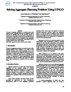
complete as possible to be used by and motion planning algorithms. Since the number of cells that is used to describe a real environment is normally high, not only should the attributes that are assigned to each cell be as small as possible, but it also must contain sufficient information such that the modeled cells could be used in motion planning algorithms. To do this, in this paper, 3 characteristics are assigned for each cell of the model. These attributes are as follows: 1. Horizontal distance of the cell, namely X 2. Vertical distance of the cell, namely Y 3. Occupation attribute of the cell, namely OccMem Now if the appropriate a number of above cells is arranged in a matrix form, they will present a suitable robot’s environment model. Notice that in the presented model, every point of the real environment can only be mapped into a single cell. A membership function, moreover, is used to assign an appropriate belief value for each real environment cell. This membership function is designed so that it returns 0.0 (case (a) of Figure 1) for the real environment cells with no obstacle, 1.0 (case (b) of Figure 1) for the real cells with an obstacle, and a value between [0,1] for the real cells with ambiguity of the presence of the obstacle according to the cell’s uncertainty. Referring to the model described above, the OccMem is the variable that represents the cell uncertainty due to the possibility of presence an obstacle in a cell. To show how the uncertainty is modeled in this approach, suppose the real environment is like Figure 2, and the cell uncertainty is up to 10 cells. In this case, if we consider the triangular Real Cell
Model Cell
(a)
Real Cell
Model Cell
(b) Figure 1: Cellular Modeling
µ (x)
x
Figure 2: Initial Robot Environment
Figure 4: Fuzzified Initial Robot Environment
-10 +10 Figure 3: Membership function of cell’s uncertainty
Figure 5: Eight possible cells for a Mobile Robot
occupation membership function as shown in Figure 3, the final environment model would be generated as Figure 4. IV. SOLVING THE MOTION PLANNING PROBLEM The next step in solving the motion planning problem, after modeling the environment, is to model for the main problem and parameterize its input and output relationships. In section 1, Hopfield N.N. was described; and now, the motion planning problem should be parameterized so that its parameters are matched to Hopfield N.N. formulation. In the case being considered here, three states are used totally. Two of the states are horizontal and vertical distances between the current and the target robot positions, and the last one is the cell’s uncertainty of the current robot position. Referring to Hopfield N.N. energy function (4), we have: 3 1 3 3 E = ∑∑ wij xi x j + ∑ I i xi (5) 2 i =1 j =1 i =1 In this case, equation (5) can be rewritten as: x1 1 E = x2 2 x3
T
w11 w 21 w31
w12 w22 w32
w13 x1 I1 w23 x2 + I 2 w33 x3 I 3
T
x1 x 2 x3
(6)
Now if we assign the parameters of the equation (6) like: w11 w12 w21 w22 w31 w32
T
w13 2 0 0 I1 0 w23 = 0 2 0 , I 2 = 0 I 3 10 w33 0 0 0
T
(7)
Then, the final energy function could be summarize as follows:
(
) (
E = x12 + x 22 = xCurrent − xTarget
) + (y 2
+10 × Uncertaint y (x1 , x2 )
Current
− y Target
)
2
(8)
Notice that, the final energy function described in (8) is proportion to the square of the distance between the current and the target robot positions. It is obvious that the energy of farther positions is larger than that of the nearer ones, and when the robot reaches its target, the energy will be absolutely zero. Another feature that should be mentioned here, is the uncertainty factor placed in the Hopfield N.N. energy function. Notice that, the energy function of a cell is incremented according to the uncertainty of the cell. As a result, the Hopfield N.N. is designed in a way that it selects the cells with less uncertainty in its optimization process. Now the robot’s environment should be fed into Hopfield N.N.; therefore, the second step is adapting the Hopfield N.N. with the real environment model. According to the real environment modeling that divides the real environment into individual cells, the center of the robot is considered to be in one of the model cell at any instant of time. Referring to Figure 5, there are 8 possible cells for the robot that it can move into at its next control iteration. Thus, an appropriate algorithm should be designed to 0-7803-7280-8/02/$10.00 ©2002 IEEE
choose the best cell for the next move. To catch the goal, the simplest algorithm can be described as follows: 1. Deleting the cells that an obstacle is placed in 2. Calculating the energy of the remaining cells 3. Moving toward a cell that has the least energy value 4. Repeating stages 1 through 3 until the robot reaches its target position Notice that by using predefined techniques to model the problem as an energy function and try to optimize (minimize) it, the motion planning problem has been reduced to an optimal control problem. Hence, like most optimization algorithms, attractors trap our algorithm too. Therefore, five ideas (methods) have been put into use in this optimization algorithm to escape from the attractors and get rid of them. These ideas, sorted at the degree of importance, are listed as follows: 1. Choosing optimal weights of I’s and W’s 2. Moving with respect to the prediction of the moves to come 3. Avoiding repeated moves 4. Saving the attractors and local minima 5. Adjusting the prediction level A. Choosing optimal weights of I’s and W’s Having an over look on the subjects described in section 2, the only criterion for optimization in Hopfield N.N., is its energy function. Thus, choosing optimal weights for the energy function plays the vital role in Hopfield N.N. optimization process. So, the algorithm will be safer of getting trapped by many attractors and local minima when the optimal weights are chosen. In this case, the weights of I’s and W’s are chosen as it is given in equation (7). B. Moving with respect to the prediction of the moves to come Although by choosing the optimal weights for I’s and W’s for Hopfield N.N., which is usually used to solve optimization problems, getting trapped by many attractors can be avoided, some attractors still remain and escape from them may be inevitable. Thus, the second trick in solving this optimization problem is the prediction of the moves to come. To do this, regarding to a predefined depth, before any move, the next possible moves of the robot are evaluated; then, the robot, in each control iteration, chooses direction toward a cell that generates the least energy in the next moves. C. Avoiding repeated moves Another algorithm, which is used by Hopfield N.N., is an algorithm that prevents the main optimization process from repeated moves. To describe this auxiliary algorithm, suppose that the robot is in a cell and wants to make a decision for its next move. Also suppose that the cell, chosen as the best, was passed through by the robot before. In this case, if the robot selects the cell and moves toward it, it will certainly get trapped into an idle loop! So, it is
wise to purge this kind of cells and do not move into them. Because, we would never reach to a cell again if it were a part of the actual optimized route. Therefore, to avoid getting trapped by this kind of cells, Hopfield N.N. uses another algorithm to aware itself from these repeated moves in every occasion that the robot wants to move into a cell. This auxiliary algorithm saves the current cell into a Link List structure. Hence, all the cells the robot moved into step by step, to reach the target, are saved sequentially. Finally, in each control iteration, the robot first searches this Link List, and when it assures that the selected cell has not been repeated before, it chooses it as its next cell to go. D. Saving the attractors and local minima The fourth algorithm that is used by Hopfield N.N. is an algorithm that finds the attractors and saves them into another Link List structure. With the help of this Link List, every attractor can trap the main algorithm only once. The way that the algorithm recognizes an attractor is very simple. Suppose that the robot is in a cell with coordinates ( x0 , y 0 ) with corresponding energy value E0 . Also suppose that the best cell for the robot, for the next move, is ( x1 , y1 ) with corresponding energy value E1 . Now, if E1 is being greater than E0 ( E0 < E1 ), then the current robot position is certainly an attractor. In other words, in each control iteration, if the energy of the next cell is greater than the current position’s energy value, the current cell is an attractor. At last, before choosing a cell as the next move position, the robot searches it on this Link List. If the selected cell does not exist in the Link List, it is chosen for the next move to go. E. Adjusting the prediction level The last auxiliary algorithm that is used to improve the optimization procedure is an algorithm that adjusts the prediction level for the main algorithm. As a matter of fact, by using the prediction criteria, we eliminate some cells in the modeled environment. That is, having greater level of prediction will eliminate more cells. Thus in some occasions, it is possible that no cell remain for the robot to move. In such cases, the prediction level will decrease one level, and the main algorithm is launched, from the beginning, again. V. TESTING THE ALGORITHM To show the ability of combination of auxiliary algorithms and the Hopfield N.N., suppose that the real environment is like Figure 6 and it is divided into 400× 300 individual cells. Also, suppose that start and target robot positions are (10,10) and (390,290) , respectively. In this case, the proposed algorithm solves the problem successfully, but referring to Figure 6, the final answer is obviously not optimal and need to be optimized. Therefore, another algorithm should be designed to optimize the answer. 0-7803-7280-8/02/$10.00 ©2002 IEEE
VI. OPTIMIZING THE FINAL ANSWER The last stage in solving a motion planning problem is to optimize the obtained rough result. In this case, optimization is equivalent to find a path with the shortest length between start and target robot positions. Since the Hopfield N.N. usually generates answers with long streams, an appropriate optimization procedure for improving the final Hopfield N.N. result is necessary. With respect to the problem, two similar algorithms can be recommended. In both cases, the optimization algorithm tries to find two points (positions) in the answer stream that have direct sight to each other. Consequently, if all this kind of cells, having direct sight to each other, is being found and connected by a shortcut, the final answer will certainly be shorter than before. For example, in Figure 6, although two points marked as A and B have direct sight to each other, they didn’t connect to each other directly. Thus, if we create a shortcut between these two points, the final path would become shorter. Two algorithms designed to optimize the final answer are as follows: 1. Optimizing the path from Head to Tail. 2. Optimizing the path from Tail to Head. A. Optimizing the path from Head to Tail In the algorithm that optimizes the answer from Head to Tail, the methodology is to begin from the start point and try to find the farthest point having direct sight to it. Now, if we move to the second point, after creating a shortcut, and do the same procedure to find shorter paths, the final answer will be more optimal and shorter than the first one. The methodology of Head to Tail optimizer is implemented as follows: Step 1: Let N be the length of the answer stream generated by Hopfield N.N.; and also, let X (i);i = 1 ,..., N be the i th element of the answer stream. Step 2: Let k = 1 . Step 3: Find X ( j ) for j = N down to k , which has direct sight to X (i ) and the sum of the intermediate cell’s uncertainty is less than 2.0 . Step 4: Create a shortcut between X (i ) and X ( j ) . Step 5: Repeat steps 3 through 4 with k = j , until the target point of the answer stream i.e., k = N . B.
Optimizing the path from Tail to Head The second algorithm used to optimize the answer obtained by the Hopfield N.N., is an optimization procedure that tries to optimize the answer from Tail to Head. This new algorithm is similar to the optimizer from Head to Tail; and, the only difference between them is due to their searching direction. Unlike the first algorithm, this new method starts from the target and tries to find the farthest point (from the start) having direct sight to it. Continuing this procedure for all the points of the path, the length of the final answer will be shorter than that of the first one. The
methodology of Tail to Head optimizer is implemented as follows: Step 1: Let N be the length of the answer stream generated by Hopfield N.N.; and also, let X (i);i = 1 ,..., N be the i th element of the answer stream. Step 2: Let k = N . Step 3: Find X ( j ) for j = 1 to k , which has direct sight to X (i ) and the summation of cell’s uncertainty is less than 2.0 . Step 4: Create a shortcut between X (i ) and X ( j ) . Step 5: Repeat steps 3 through 4 with k = j , until the start point of the answer stream i.e., k = 1 . C. Choosing Optimization methodology To show how these two algorithms are difference, assume we want to optimize the answer obtained in Figure 6 by these two optimizers. The results of the Head to Tail and Tail to Head optimizers are shown in Figures 7 and 8 respectively. Referring to Figures 7 and 8, although the optimized answers are much better than the answer shown in Figure 6, there are still some points that still have direct sight (points A and B in Figure 7, and C and D in Figure 8) to each other; that is, the final path can be shorter. Therefore, another algorithm to optimize this kind of paths should be designed and implemented. The final presented algorithm is the combination of the above two algorithms. In this new optimizer, the answer obtained by the Hopfield N.N. is optimized in two steps. First, the answer is optimized by the Tail to Head optimizer; then, the result of
the first step is optimized by Head to Tail optimizer. The final algorithm can be summarized as follows: 1. Input the robot’s environment model 2. Input the robot start and target positions 3. Using Hopfield N.N. to solve the problem, the answer is named m_Moves 4. Optimizing the answer obtained in step 3 (m_Moves) from Tail to Head, the answer is named m_SubOptimal 5. Optimizing the answer obtained in step 4 (m_SubOptimal) from Head to Tail, the answer is named m_Optimal Notice that the final algorithm takes the robot start and target positions, and the model of the robot’s environment and generates the final answer (m_Optimal) between the robot start and target positions. To show how the above algorithm works, suppose we want to optimize the answer depicted in Figure 6. Figure 9 shows the final path that is obtained by launching the final combined optimizer. It is worth mentioning that in almost all cases the obtained answers from any of the above optimizers are fully optimized and there is no need to launch the combined optimizer. But to show the necessity of the combined algorithm, the example selected in Figure 6, a special case, has some properties that none of the above algorithms can optimize it thoroughly. As another example, consider the robot’s environment as in Figure 10, while the robot start and target positions are (10,10) and (390,290) respectively. It can be seen that the path computed by the final proposed algorithm is fully optimal and it cannot become shorter anymore. Notice that, although there exist some deep Utraps in robot’s environment, the algorithm never gets
Figure 6: The initial answer obtained by the Hopfield N.N
Figure 7: Optimizing the path in Figure 6 by Head to Tail optimizer
Figure 8: Optimizing the path in Figure 6 by Tail to Head optimizer
Figure 9: Optimizing the path in Figure 6 by combined optimizer
Figure 10: A robot environment with deep U-traps
Figure 11: A robot environment with deeper U-traps
0-7803-7280-8/02/$10.00 ©2002 IEEE
trapped by them. Figure 11 is another example with really hard constraints and very deep U-traps. In this figure robot start and target positions are (10,10) and (220,240) respectively, while the cell’s uncertainty is up to 10 cells.
References:
VII. CONCLUSION In this paper, a new method for solving various kind of robot motion planning Problems is presented. As it has been shown, the algorithm is intelligent and can be useful even in the presence of very complex environments. Since the rough method of using the Hopfield N.N. cannot solve complex problems, some auxiliary algorithms are designed to work with the Hopfield N.N. optimizer to find the answer in all the cases. However, since the obtained answer by the Hopfield N.N. is usually sub-optimal, it should be optimized. So other algorithms to optimize this answer are designed and implemented; “Head to Tail” and “Tail to Head” optimizers. The optimizers are designed and tested, but there have been some occasions that none of the above optimizers could find the optimal answer completely. Therefore, another optimizer, which is obtained from the combination of the above two algorithms, has been designed and implemented. Finally, an algorithm is presented which takes the robot start and target positions and its modeled environment to compute the optimal path. Even in presence of deep U-traps, the optimal path links start and target positions with the shortest existing path. Another feature, which has been presented in the proposed algorithm, is to consider and model the cell uncertainty into the Hopfield N.N. energy function for fuzzifying the robot’s environment. By means of this approach, the Hopfield N.N. optimizer is forced to choose the cells with less uncertainty in its optimization process. Having this feature makes this approach to be really different from other methods in solving the robot motion planning problems, like the approach presented in [7]. Although the proposed algorithm is applied to the robot motion-planning Problem, it can also be used for any other optimization problem having very hard discrete constraints.
[3]
0-7803-7280-8/02/$10.00 ©2002 IEEE
[1] [2]
[4]
[5]
[6]
[7]
[8]
[9] [10] [11]
[12] [13] [14] [15] [16] [17]
[18]
J.T. Schwartz, M. Sharir, “A Survay of Motion Planning and Related Geometric Algorithms”, 1997. Sundar, Z. Shiller, “Optimal Obstacle Avoidance Based on the Hamilton-Jacobi-Bellman Equations” , IEEE Trans. on Robotics and Automation, Vol. 13, No. 2, 1997. Maeda, M. Tanabe, M. Yuta, T. Takagi, “Hierarchical Control for Autonomous Mobile Robots with Behavior-Decision Fuzzy Algorithm”, Proceeding of IEEE International Conference on Robotics and Automation, 1992. R. Beom, H. S. Cho, “A Sensor-Based Navigation for a Mobile Robot Using Fuzzy Logic and Reinforcement Learning”, IEEE Trans. on Robotics and Automation, Vol. 25, No. 3, 1995. M. Brown, R. Fraser, C.J. Harris, C.G. Moore, “Intelligent SelfOrganizing Controllers for Autonomous Guided Vehicles, Comparative Aspects of Fuzzy Logic and Neural Nets”, IEE Conference Publication, Vol. 1, No. 332, pp 134-139, 1991. W. Li, “Perception-Action Behavior Control of a Mobile Robot in Uncertain Environments Using Fuzzy Logic”, Proceedings of IEEE Conference on Intelligent Robots and Systems, 1994. N.Sadati, J. Taheri, "Hopfield Neural Network in Solving the Robot Motion Planning Problem", IASTED International Conference on Applied Informatics (AI2002), Innsbruck, Austria, February 18-21, 2002. N.Sadati and J.Taheri “Hopfield Neural Network in Solving the Puzzle Problem”, 26th International Conference on Computers and Industrial Engineering, Melbourne, Australia, Dec 1999. H.Schildt, Artificial Intelligence Using C, McGraw-Hill, 1987 K.A. Bowen, Prolog and Expert Systems, McGraw-Hill, 1991. H.P.Schwefel, R.Manner Eds. Parallel Problem Solving from Nature- Proc 1st workshop PPSN1, Vol 496 of lecture, Noted in Computer Science, Berlin, Germany. Springer 1991. H.P. Schwefer, Numerical Optimization of Computer Models, John Wiley, Chichester, 1981. J. Hopfield, D.Tank, Computing with Neural Circiuts; A Model, Science 233, 1986. J. Hopfield, D.Tank, Neural Computation of Decision in Optimization Problem, Biological Cybernetics, Vol 52, 1985. S.Y.Kung, Digital Neural Networks, Prentice Hall, N.J., 1993. P. Arabie, L.J. Hubert, G.De Soete, Clustring ans Classification, World Scientific Publishing Co. Pte. Ltd, 1996. Kebi B. Irani, Suk I. Yoo, “A Methodology for Solving Problems: Problem Modeling and Heuristic Generation,” IEEE Trans. on Pattern Analysis and Machine Intelligence, Vol. 10, No. 5, September 1988. Q. S. Gao, H. D. Cheng, Macro Transform Approach to Solve Indecomposable Problems, IEEE International Computer Society Press, 1989.