Solving Steel Mill Slab Problems with Constraint-Based Techniques ...

Solving Steel Mill Slab Problems with Constraint-Based Techniques: CP, LNS, and CBLS Pierre Schaus Dynadec, Belgium [email protected]

Pascal Van Hentenryck Brown, US [email protected]

Jean-No¨el Monette UCLouvain, Belgium [email protected]

Carleton Coffrin Brown, US [email protected]

Laurent Michel UCONN, US [email protected]

Yves Deville UCLouvain, Belgium [email protected]

June 15, 2010 Abstract The Steel Mill Slab Problem is an optimization benchmark that has been studied for a long time in the constraint-programming community but was only solved efficiently in the two last years. Gargani and Refalo solved the problem using Large Neighborhood Search and Van Hentenryck and Michel made use of constraint programming with an improved symmetry breaking scheme. In the first part of this paper, we build on those approaches, present improvements of those two techniques, and study how the problem can be tackled by Constraint-Based Local Search. As a result, the classical instances of CSPLib can now be solved in less than 50ms. To improve our understanding of this problem, we also introduce a new set of harder instances, which highlight the strengths and the weaknesses of the various approaches. In a second part of the paper, we present a variation of the Steel Mill Slab Problem whose aim is to minimize the number of slabs. We show how this problem can be tackled with slight modifications of our proposed algorithms. In particular, the constraint-programming solution is enhanced by a global symmetric cardinality constraint, which, to our knowledge, has never been implemented and used before. All the proposed approaches to solve this problem have been modeled and evaluated using Comet.

1

1

Introduction

The steel mill slab problem is to assign colored sized orders to slabs of different capacities such that the total loss is minimized and at most two different colors are present in each slab. The CSPLib instance (111 orders, 88 colors, 20 capacities) of this problem remained unsolved for years until 2007 when Gargani and Refalo introduced an elegant constraint programming (CP) model. They solved the instance optimally (i.e., with zero loss) with a Large Neighborhood Search (LNS) in 3 seconds [3]. Recently, Van Hentenryck and Michel showed that a pure CP approach can solve the problem in less that 7 seconds if one breaks value symmetries during search [5]. In the first part of this paper, we compare three approaches to the steel mill slab problem: CP, LNS, and Constraint-Based Local Search (CBLS). It appears that the CSPLib instance is no longer challenging, since a very simple CBLS model in Comet is able to solve it optimally in less than 0.05 second. This outperforms all the previous attempts to solve this problem. For this reason, we propose a new set of 380 instances with increasing difficulty derived from the CSPLib instance. We compare the three approaches (CP, LNS, and CBLS) on these new instances. In the second part of the paper, we propose a variant of the problem with a different objective function. Manipulating slabs is a heavy task in the steel industry and hence limiting the number of slabs is also desirable in practice. We propose to minimize the number of used slabs such that the loss does not exceed a given value (typically the minimum loss). We propose a CP model for this new problem exploiting the global symmetric cardinality constraint [6] (sym-gcc) which enables us to solve many instances that would be intractable otherwise. To our knowledge, this is the first time that the sym-gcc constraint is implemented and used in practice1 . Related Work and Existing Results Beside previous unsuccessful tentatives (e.g., [12]) to solve efficiently the Steel Mill Slab Design Problem, Gargani and Refalo [3] presented in 2007 a CP model that takes advantage of the structure of the problem through global constraints. They solved the problem in 3 seconds using a specific heuristic for variable and value selection and combining it with LNS. They also considered the use of static symmetry breaking constraints but it negatively influenced the search for large instances. More recently, Van Hentenryck and Michel [5] showed how dynamic symmetry breaking could improve the search. Doing so, they were able to solve the CSPLib instance in less than 7 seconds with an exact search procedure. Outline The remainder of this article is as follows. Section 2 introduces the problem and the instances. The subsequent sections (3 to 7) present the various models and search procedures, together with their experimental results. Section 8 deals with the slab minimization variant. Section 9 concludes the paper. 1 The

sym-gcc is available into Comet [2] under the name setGlobalCardinality constraint

2

2

The Steel Mill Slab Problem

Steel is produced by casting molten iron into slabs. A steel mill can produce a finite number of slab capacities. An order has two properties: a color corresponding to the route required through the steel mill, and a size. Given n input orders, the problem is to assign the orders to slabs such that the total size of steel produced is minimized [1]. This assignment is subject to two further constraints: 1. Capacity constraints: The total size of orders assigned to a slab cannot exceed the largest slab capacity. 2. Color constraints: Each slab can contain at most 2 colors. The color constraints arise because it is expensive to cut up slabs in order to send them to different parts of the mill. Example Figure 1 shows the solution of a small instance with three possible slab sizes (5, 6 and 8), 6 orders, and 3 different colors. Each order is represented by a vertical bar whose height is the size (also indicated inside the rectangles). It can be seen that there are at most two different colors in each slab. The cost of this solution is 1, as there is 1 unit of steel wasted in slab S3. Indeed, only 4 units are used but the smallest slab size is 5. Empty slabs (S4 and S5) do not incur costs or benefits.

Figure 1: A Small Example of the Steel Mill Slab Problem. There exists only one available real instance for this problem, available in the CSPLib2 . We now describe some characteristics and measures about this instance, before presenting the new instances.

2.1

The CSPLib Instance

The CSPLib instance is composed of 111 orders with a total of 88 different colors. In the CSPLib instance, 20 slab capacities are available. They are in 2 http://www.csplib.org/prob/prob038/111Orders.txt

3

increasing order: 12, 14, 17, 18, 19, 20, 23, 24, 25, 26, 27, 28, 29, 30, 32, 35, 39, 42, 43, 44. For a color c, let Oc denote the set of orders having color c. In the CSPLib instance, the cardinality of such a set never exceeds 4 for any color. The following table report the number of sets with cardinalities 1 to 4: cardinality of color sets number of color sets

1 71

2 13

3 2

4 2

Since very few orders have the same color, it seems natural to think that the constraint at most two colors are present in each slab will give a lot of information. For instance, if two orders among the 71 sets with a unique color are placed in the same slab, we immediately know that none of the 109 remaining orders can be placed in this slab. Note that, from this original instance, 100 sub-instances were considered in [3, 5] by only including the first 12, 13, . . . , 111 orders respectively. This allowed these papers to study the behavior of the algorithm as the problem size increases.

2.2

Generation of New Instances

A fundamental observation on this problem is that the higher the density of the slab capacities, the easier the problem becomes. This is because, in each slab, many combinations of orders can give a loss of 0. The CSPLib instance has 20 slab capacities ranging from 12 to 44. Furthermore, two large blocks of consecutive slab capacities are present ([17..20] and [23..30]) making it very easy to obtain a loss of 0 in a slab. This explains why the CSPLib instance can be solved without any difficulty. We propose to add complexity to the CSPLib instance by generating new slab capacities without changing the set of the 111 orders. To keep characteristics close to the original instance, the slab capacities are uniformly randomly generated between 10 and 50. We generated instances with a number of possible capacities varying between 2 and 20. For each number of capacities, 20 instances were created making a data set of 19 × 20 = 380 instances of increasing difficulty (as the number of capacities decreases). We ensure that all problems are feasible, i.e., that the largest slab capacity was at least as large as the largest order size. When the number of capacities decreases, the probability of reaching a loss of zero decreases. This creates instances with an additional interesting challenge, as the optimality proof may now become non-trivial. These new instances and our best results (see Section 7) are available at the url: http://becool.info.ucl.ac.be/steelmillslab. We also plan to maintain any future improvement made on these instances.

3

The Model

To solve the steel mill slab problem, this paper considers three constraint-based techniques (CP, LNS, CBLS), which are all based on the same high-level model, which captures the combinatorial substructures of this application. This section 4

presents the common model, while the three following sections show how this model will be used differently by the various approaches. The model used in this work is based on Gargani and Refalo [3]. Let n be the number of orders. The color of order o ∈ [1..n] is denoted by color(o) and its size by size(o). Let m be the number of available slabs (if there is no constraint on the S number of available slabs we can set m = n without restriction). Let C = o∈[1..n] {color(o)} be the set of colors. Let Oc be the set of orders with color c (c ∈ C). For an order o ∈ [1..n], Xo is a variable denoting the slab assigned to order o. The domain of Xo is the interval [1..m] of slab indices. W The following expression indicates whether color c is used in slab i: o∈Oc (Xo = i). The constraint that at most two different colors are present in a slab is: ! X _ ∀i ∈ [1..m], Xo = i ≤ 2, (1) c∈C

o∈Oc

in which a boolean expression has value 1 when true and 0 otherwise. For each slab j ∈ [1..m], a load variable Lj indicates the total size of the orders assigned to this slab. These variables are linked to order variables with the set of constraints: X ∀j ∈ [1..m], Lj = size(o). (2) o∈[1..n]:(Xo =j)

With each slab j ∈ [1..m] comes a loss variable Fj (free space available in slab j). Since the objective is to minimize the available free space3 , Fj is the minimum possible free space available in slab j. This minimum free space is obtained from Lj by choosing the smallest slab capacity larger or equal to Lj . The available slab capacities4 are capa = {0, c1 , . . . , cp } with 0 < c1 < . . . < cp . The possible free spaces are precomputed in an array F for all possible load values l: ∀l ∈ [0..cp ], F[l] = min{c − l | c ∈ capa ∧ c ≥ l}. This is well defined as we assume cp ≥ maxo∈[1..n] size(o). The free space of slab j is written with P an element constraint as Fj = F[Lj ]. The objective to minimize is j∈[1..m] Fj that is the total loss. Although there is no explicit variable telling the capacity chosen for a slab j, this can be easily deduced as Lj +Fj . The model also replaces the set of constraints given in Equation 2 by the global packing constraint Pack which enables more propagation in CP [10] and more incrementality in CBLS.

4

Constraint Programming

The CP solution uses the above model with the heuristic from [5]. The search procedure selects the order with the smallest domain to assign next. Ties are broken by preferring the largest order. 3 This is equivalent to minimizing the total steel produced as the consumed part is constant P and equal to o∈[1..n] size(o). 4 We introduce the capacity of 0 to allow empty slabs.

5

4

5

CP−DSB CP−DSB−VAL

●

●

time (s)

3

●

●

●

●

2

●

●

● ● ●

1

● ●

●

●

●

0

●

●

●

●

20

●

●

●

●

●

●

●

40

●

●

●

●

●

●

●

60 number of orders

80

100

Figure 2: Experimental Results of CP on the CSPLib Instance.

4.1

Dynamic Symmetry Breaking (DSB)

The Steel Mill Slab problem exhibits value symmetries since every non empty slab is interchangeable with an empty slab in the final solution. These symmetries can be avoided during the search by considering only one empty slab for each order variable. In other words, when an order variable Xi is chosen for assignment, only non-empty slabs and one empty slab should be considered as possible values for Xi . This search procedure is due to [5] and allows to solve the CSPLib instance in less than 10 seconds.

4.2

Value Heuristic (VAL)

None of the models presented in [3, 5] make use of a specific value heuristic. They try to place the orders from the smallest slab index to the largest slab index. We propose to try the slabs increasingly according to the loss increase induced into that slab for the partial solution if the order is placed into it. The idea is to keep the loss of the partial solution as small as possible (as we would do for a greedy search). This value heuristic is evaluated against the default labeling heuristic used in [3, 5].

4.3

Experimental Results on the CSPLib Instance

In this section, we analyze the behavior of the CP Model using Comet [2] on the 100 instances of CSPLib. Figure 2 compares the execution time of the model from [3] using the dynamic symmetry breaking (DSB) heuristic of [5], with and

6

without our value heuristic (VAL). As can be observed, the value heuristic has a real positive effect. For the largest instance: 2251 backtracks and 5 seconds are necessary without the value heuristic, against only 1434 backtracks and less than 3 seconds using it.

5

Large Neighborhood Search

Large Neighborhood Search (LNS) [9] is the idea of using constraint programming to improve an existing solution. More precisely, given a solution, LNS freezes a part of the solution and searches for new assignments to the remaining variables (the fragment). The chosen neighbor is found by solving this reduced problem with CP (with the strategy described in Section 4 using the value heuristic DSB-VAL). A limit is generally given to improve the current solution by solving the reduced problem. If no better solution can be found upon this limit, the variables of the fragment are restored to their previous values and the process is repeated again.

5.1

Experimental Results on the CSPLib Instance

As suggested in [3], we use fragments constituted of a random subset of the X1 , . . . , Xn variables. We experimented with two cardinality policies to choose the fragment size: 1. a cardinality chosen randomly between 50 and 95% of n (as in [3]), and 2. a cardinality chosen randomly between 5 and 10 orders. The limit is set to 60 failures as in [3]. The search used is identical to Section 4 with the dynamic symmetry breaking and the value heuristic. Figure 3 reports the average time for 100 runs with each of the two cardinality policies. Dashed lines represent the average ± the standard deviation. It appears that choosing smaller fragment sizes (between 5 and 10 orders) decreases the time to find the optimal solution. In comparison with the pure CP approach, we cannot really say that LNS is faster on these instances. Subsequent experiments (in Section 7) will show that LNS outperforms pure CP on more difficult problems.

6

Constraint-Based Local Search

Constraint Based Local Search (CBLS) [11] is the idea of performing local search on high-level models. Constraints and objectives in CBLS incrementally maintain properties such as their violations and their values, and they support queries to determine how these properties change under local moves (differentiation). We consider two approaches to solve the Steel Mill Slab problem with CBLS. Both CBLS methods operate on the model described in Section 3 but differ in the search procedure. The first approach, CBLSh , maintains a neighborhood of 7

2.5

3.0

LNS (50−95)% LNS 5−10

●

●

2.0

●

time (s) 1.5

● ● ●

1.0

●

●

● ●

0.5

●

0.0

● ●

●

●

20

●

●

●

●

●

●

● ●

40

●

●

● ●

●

●

●

●

●

●

●

60 number of orders

80

100

Figure 3: Experimental Results of LNS on the CSPLib Instance with Two Different Fragment Size Policies. feasible assignments and only considers local moves which maintain feasibility. In other words, this model considers that all constraints are hard. The second approach, CBLSs , considers both feasible and infeasible assignments and uses an objective function that combines the loss and the constraint violations. In this model, all constraints are soft and the objective drives the search towards feasible assignments. For the two approaches, there are many decisions to make, and parameters to tune. Here are the main choices to perform: • Neighborhood: Do we only use the move of a single order from one slab to another one, or do we allow swaps between two orders as well? • Greediness of the moves: To reduce complexity, we choose the move to perform in two steps. First, an order is chosen and given that order, a slab to move it to or another order to swap it with, is selected. We have to decide how the first order is chosen (one inducing a largest cost or at random), and how the slab or the second order is chosen (the one producing the largest improvement, or anyone producing some improvement). • Use of metaheuristics: We considered the use of periodic restarts and of tabu search. For each metaheuristic, different parameters must be chosen. To settle on a choice, we ran experiments on a small subset of the newly generated instances, exploring different combinations. The following two subsections detail the resulting search procedures. 8

6.1

CBLSh (Hard Constraints)

In the CBLSh model, the constraints of the problem (maximum capacity and number of colors for each slab) are always satisfied during the search. An initial solution is constructed to be feasible (one order per slab) and the neighborhood is defined by all assignments which maintain feasibility. More precisely, the neighborhood of a given assignment is composed of all the assignments where all orders but one remain unchanged and the remaining order is placed in another slab without violating the capacity and color constraints of this slab. For each order, the set of slabs where it can move is maintained incrementally using invariants, which allows this tightly defined neighborhood to be calculated with minimal overhead. We also tried to allow the swap of two orders. This neighborhood is larger and should lead to good solutions faster. However, the verification of the feasibility of those moves is time-consuming, and the potential benefits are lost by the lower number of moves that can be performed in a given amount of time. As this is an important design decision, we ran the two algorithms (with and without swaps) on the whole new set of instances, with a time limit of 5 minutes. Without swaps, the search reaches the best known solution for 521 instances, and for only 500 with the swaps. The total deviation from the best known solutions is also better without swaps: 626 units without swaps and 856 with swaps. It is however interesting to note that the swaps improve the results for the difficult problems with only two slab sizes. The search is semi-greedy. On even iterations, a slab with a positive loss is randomly chosen. On odd iterations, a slab with the largest loss is chosen. An order in the selected slab is randomly chosen. The chosen order is then moved to the best among the possible slabs (obtaining the largest decrease of the total loss). We experimentally observed that, with greedy moves only, the search quickly converges to a local optimum and becomes stuck. On the contrary, with only semi-random moves, the search does not converge towards good quality solutions. Alternating the two approaches proved to be a good compromise between intensification and diversification. In addition, this semigreedy search is diversified through two mechanisms: a totally random move every 20 iterations and a full restart every 5000 iterations. These parameters have been fixed experimentally.

6.2

CBLSs (Soft Constraints)

The CBLSs model assigns weights to the constraints and to the objective in order to drive the search towards feasible assignments. The feasibility constraints are given an arbitrarily large weight while the objective is given a weight of one. An initial assignment is constructed by randomly placing two orders on each slab (this ensures the color constraint is initially satisfied). The neighborhood consists of assigning an order to a new slab and of swapping two orders. Moves assigning a singleton order to an empty slab and swapping two singleton orders are not considered. For this search approach, swaps have been shown to be

9

l1 o1

size(o1)

slab capacities

l2

s1

s2

Figure 4: Illustration of the Differentiation of the Objective useful. As the constraints are soft, the feasibility of the move should not be checked. There was thus no real overhead in enlarging the neighborhood. The search is semi-greedy and uses a tabu component. On even iterations, a greedy move is performed. The order with the most impact is selected, all moves (assignments or swaps) involving the chosen order are considered, and the move minimizing the violations is selected. On odd iterations, a semi-greedy move is made. An order is selected at random and is assigned to a new slab which minimizes the objective value. As for CBLSh , this odd/even mechanism follows from a need to balance intensification and diversification. In addition, the search is diversified after 10,000 iterations without improvement. The diversification procedure is as follows: select 1/7 of the slabs at random and, for each such slab o, select a new slab d at random and place the orders from slab o onto slab d. This causes a number of violations of the maximum capacity and color constraints but they are quickly resolved by the greedy steps. It was observed that a greedy search procedure rarely uses the largest slab capacities and this diversification was designed to help the search discover order configurations using the largest slab sizes. Again, the details of the algorithm have been calibrated by experiments on a subset of the generated instances.

6.3

Differentiation in CBLS

Both CBLS models rely on differentiation to guide their search. Here we provide a simple example of differentiation to illustrate what is happening. Consider an order o1 of size size(o1) in slab s1 which has a current load of l1. Consider the effect of moving o1 in slab s2 (which is computed by method getAssignDelta(o1,s2) in Comet), that is how the total loss would change if the order o1 were moved to slab s2. This is illustrated on Figure 4. Assume that the current load of the slab s2 is l2 and recall the precomputed table of the losses as function of the loads (table F in Section 3). The current loss of these two slabs is F[l1]+F[l2]. Now, if the order o1 is moved to slab s2, the loss of these two slabs becomes F[l1-size(o1)]+F[l2+size(o1)]. The loss of any other slab does not change. Hence getAssignDelta(o1,s2) returns in constant time the value F[l1-size(o1)]+F[l2+size(o1)]-(F[l1]+F[l2]). 10

3.0

CBLSs CBLSh

0.0

0.5

1.0

time (s) 1.5

2.0

2.5

●

●

●

●

20

●

●

●

●

●

●

●

40

●

●

●

●

●

●

●

●

●

●

60 number of orders

●

●

●

●

●

●

●

80

●

●

●

●

●

●

100

Figure 5: Result of the Two CBLS Comet Models on the CSPLib Instance. In the CBLSh model, the differentiation of the objective is used to guide the search to optimality via feasible neighbors. In the CBLSs model, the differentiations of the constraints and the objective are carefully composed to give every neighbor a unique rank and to drive the assignment towards both feasibility and optimality.

6.4

Experimental Results on the CSPLib Instance

To solve the largest instance with 111 orders, the CBLSh model needs on average 50 iterations and less than 50ms. This outperforms significantly any previous approaches and does not require any special meta-heuristic. Figure 5 depicts the same experiment as for the CP and LNS models on the 100 instances derived from the CSPLib instance. Since the CBLS searches are also stochastic, the results are averages for 100 runs. The dashed lines reports the average ± the standard deviation. The results of CBLSh are very impressive since the time never exceeds 0.05 seconds and are reasonably stable. The CBLSs model is slower and obtain running time more comparable (up to 2.5 seconds) to LNS. We will see later on that CBLSs obtains smaller total loss than CBLSh on really difficult instances.

7

Comparison of CP, LNS, and CBLS

We now compare the three approaches on the set of the 380 newly generated instances. On these new instances, the total optimal loss found is not always 0.

11

Table 1: Value of the minimum loss found for each instance # capas 0 1 2 3 4 5 6 7 8 9 10 11 12 13 14 15 16 17 18 19

2 28 64 107 41 19 50 44 44 531 76 85 78 28 104 61 296 70 162 45 45

3 6 20 13 28 9 35 19 59 77 158 49 19 7 23 18 45 40 9 35 21

4 34 24 16 12 8 6 9 3 1 15 17 10 2 22 1 15 23 0 5 13

5 0 22 6 2 13 10 0 0 4 5 8 6 20 10 2 14 5 13 21 0

6 0 22 2 0 0 2 2 0 0 1 1 7 0 17 5 5 0 0 0 1

7 0 0 3 0 4 3 0 3 0 0 7 0 2 4 0 0 0 1 0 1

8 0 0 0 0 0 0 0 0 0 0 0 0 0 6 0 0 0 0 0 0

9 0 0 0 0 0 0 0 0 0 0 0 0 4 0 0 0 0 0 0 0

10 0 0 0 0 0 0 0 0 0 0 1 0 0 0 0 0 0 1 0 0

11 0 0 0 0 0 0 0 0 0 0 0 0 0 0 0 0 0 0 0 0

12 0 0 0 0 0 0 0 0 5 0 0 0 0 0 0 0 0 0 0 0

13-20 0 0 0 0 0 0 0 0 0 0 0 0 0 0 0 0 0 0 0 0

A time-out of 300 seconds is fixed for each run on each instance and we measure the smallest loss found during this period. For one experiment, a deterministic technique is applied once per instance (CP-DSB-VAL), while the losses are averaged over 5 runs for the stochastic methods (LNS, CBLSh , CBLSs ). For a given instance i, the loss5 obtained by each technique is denoted respectively CP-DSB-VAL(i), LNS(i), CBLSf (i) and CBLSs (i). As explained in Section 2.2, there are 19 × 20 = 380 instances: 20 instances for each number of capacities ranging from 2 to 20. The difficulty of the instances increases as the number of capacities decreases. The best known solution for each instance is reported in Table 1. They were obtained by taking the minimum loss over the CP-DSB-VAL, and the 5 LNS, CBLSh , CBLSs runs with a timeout of 300 seconds for each run. One can observe that all instances with more than 13 slab capacities have a solution with a zero loss. Of course, the loss increases when the number of slab capacities decreases and the largest best loss we found was 531 for an instance with 2 slab capacities. We first computed the average deviation from the best known solution for each number of capacities and each approach. A plot of these average deviations 5 averaged

over 5 runs for LNS, CBLSh and CBLSs

12

0

Average deviation of loss from minimum loss 20 40 60 80

CP−DSB−VAL 300 LNS 300 CBLSh 300 CBLSs 300

2

3

4

5

6

7

8

9 10 11 12 13 Number of capacities

14

15

16

17

18

19

20

Figure 6: Comparison of the Different Approaches with Respect to their Average Deviation from the Best Known Objective Values. The Timeout is 300 Seconds. CP-DSB-VAL 103

LNS 301

CBLSs 302

CBLSh 328

Table 2: Number of Times that Each Technique Wins on the 380 Instances.

is reported on Figure 6. For example, assume that the best known solution for instance i is a loss of 20. Assume that CP-DSB-VAL(i) = 50, LNS(i) = 22.4, CBLSf (i) = 21.2, and CBLSs (i) = 22.4. The deviations of the minimum loss for each technique are respectively 30, 2.4, 1.2, and 2.4. Figure 6 depicts the average of these deviations for each technique over the 20 instances associated with each number of capacities (from 2 to 20). It is clear that stochastic methods outperform significantly exact method (CP-DSB-VAL). Focusing on the three stochastic methods, CBLSs seems slightly better than LNS and CBLSh for hard instances in terms of quality of the solution (Figure 6). The above presentation does not exclude the possibility that the results in Figure 6 may be heavily influenced by a very small number of instances. For this reason, we present complementary results in Figure 7 by reporting the number of instances on which a technique exhibits the best solution. More precisely, assume that for an instance i, the losses obtained are CP-DSB-VAL(i) = 10, LNS(i) = 3.6, CBLSf (i) = 4.2, CBLSs (i) = 3.6, then the counters of LNS and CBLSs are incremented by 1 while the others are not. Table 2 contains the sum over all the instances. Based on this summary of the results, we can say that CBLSh outperforms all the other techniques, since it wins most of the time.

13

20 Number of instances with best value 5 10 15 0

CBLSh 300 CBLSs 300 LNS 300 CP−DSB−VAL 300 2

3

4

5

6

7

8

9 10 11 12 13 Number of capacities

14

15

16

17

18

19

20

Figure 7: Comparison of the Different Approaches with Respect to the Number of Times it Wins. The Timeout is 300 Seconds. Nevertheless, CBLSs is the best when there are only two capacities. LNS and CBLSs perform very similarly for the remaining instances. Since stochastic techniques outperform the classical CP approach on this problem, we focus on the stochastic approaches in the rest of this section. Our goal is to analyze the behavior of the three stochastic techniques for increasing timeout values. The objective of this experiment is to discover if one technique can find good solutions faster than another one. We use exactly the same settings as for the first experiment. The timeout values are set successively to 75, 150, and 300 seconds. The results are reported in Figure 8 for average results and in Figure 9 for the number of best solutions found. The results in Figure 8 indicate that each technique finds better solutions when given additional time, but are inconclusive in showing that one technique is significantly faster than another one to find good solutions. Indeed, the three curves keep their relative positions as available time increases. From the results in Figure 9, we can notice however that with a timeout of 75 seconds, on the difficult instances with two capacities, CBLSs does not outperform LNS as it is the case with a timeout of 300 seconds. Conclusion Our experiments showed that CBLSh is the best approach for problems with 3 to 20 capacities even if CBLSs obtains more often the best solution for difficult instances with only 2 capacities. LNS is very competitive with CBLSh in terms of quality of the optimum reached and very close to CBLSs in terms of the number of best values reached. It is very surprising that LNS behaves so well compared to dedicated fine-tuned local search algorithms. Note 14

20 ●

LNS 75 LNS 150 LNS 300 CBLSh 75 CBLSh 150 CBLSh 300 CBLSs 75 CBLSs 150 CBLSs 300

0

Average deviation of loss from minimum loss 5 10 15

●

2

3

4

5

6

7

8

9 10 11 12 13 Number of capacities

14

15

16

17

18

19

20

Figure 8: Comparison of the Stochastic Techniques with Respect to Different Timeouts. also that LNS clearly outperforms the pure CP approach which obtains very poor results when the number of capacities is smaller that 18.

8

Minimizing the Number of Slabs

In this section, we propose a different problem that might be a post-processing to the minimization of the loss: Find a solution to the steel mill slab problem minimizing the number of slabs such that the total loss does not exceed a given value (typically, the minimum loss). This requirement on a solution is quite natural since it minimizes the manipulation of heavy slabs and it also minimizes the number of cuts on the slabs necessary to prepare the orders. The constraintbased model is essentially the same as the one presented in Section 3: It simply adds a constraint on the total loss and replaces the previous objective by the minimization of the number of slabs m. For this new problem, the LNS and CBLSh approaches are not appropriate because the problem is already strongly constrained by the maximum loss. Hence even finding a feasible initial solution to start LNS or CBLSh is not trivial at all. On the contrary, CP-DSB behaves very well on strongly constrained satisfaction problems. Since all the constraints are relaxed in CBLSs , it is also a good candidate to solve this problem. For these reasons, we only tackle this problem with CP-DSB and CBLSs .

15

2

5

10

15

Number of capacities

20

20 15 5

10

15 0

CBLSh 150 CBLSs 150 LNS 150 2

5

10

15

Number of capacities

20

CBLSh 300 CBLSs 300 LNS 300

0

5

10

15 10 5 0

CBLSh 75 CBLSs 75 LNS 75

Number of instances with best value

tiemout 300 seconds

20

Number of instances with best value

timeout 150 seconds

20

Number of instances with best value

timeout 75 seconds

2

5

10

15

Number of capacities

20

Figure 9: Number of Times that each Stochastic Technique Wins on the 380 Instances with 3 Different Timeouts.

8.1

Lower Bounds on the Number of Slabs

To solve the problem exactly, it is classical to solve successive satisfaction problems starting from low values of m and increasing them until a solution is found. Within such an approach, it is important to find a good lower bound to start with. We first present different lower bounds. As explained in Section 2.1, there are 88 different colors. Since at most two colors can be present in a slab, at least d88/2e = 44 slabs must be used (color lower bound). This lower bound can be improved by considering also the size of the orders. In the CSPLib instance, 4 colors have more than one order larger than the half of the maximum slab capacity (44/2=22). Because these orders are larger than 22, they must be placed in different slabs. For these 4 colors, there are 9 orders larger than 22. Hence (9-4) of these orders can be considered as having colors different from the 88 existing colors. We can consider there are 93 colors to compute a lower bound. The minimum number of slabs becomes d93/2e = 47 (color+bin-packing lower bound). In general, if a color has k > 1 orders larger than half the maximum capacity, increase the number of colors by k − 1. Do that for each color then apply the color lower bound. This lower bound is computed in O(n). Without the color and the maximum loss constraints, this problem is similar to a bin-packing problem. Hence classical bin-packing lower bounds can be used as lower bound on the number of slabs. We use the Martello and Toth’s lower bound L2 [7] which is used in the propagator of the Pack constraint [10]. For the CSPLib instance with the bin capacity of 44, L2 =41 slabs (bin-packing lower bound). A comparison of the three lower bounds is given on Figure 10. The binpacking lower bound seems to be of bad quality for this problem. The color lower bound behaves reasonably well until 60 orders. The color+bin-packing lower bound dominates the previous ones and the gap between this bound and the exact minimum is at most one on these instances. This probably means

16

50 40

●

Optimal value Color+Bin−Packing LB Color LB Bin−Packing LB

● ●

number of slabs 20 30

● ● ●

●

●

●

●

●

●

●

●

●

●

0

10

●

●

●

●

20

40

60 number of orders

80

100

Figure 10: Comparison of the Lower Bounds on the Minimum Number of Slabs on the CSPLib Instances. that the difficulty of this problem is not only due to the bin-packing component but to the conjunction of the bin-packing and the color constraints.

8.2

Improving the CP Model with a Global Symmetric Cardinality Constraint

This section improves the model by introducing a global constraint to express the color constraints allowing a stronger filtering of the domains. The following example illustrates that the filtering of the color constraints as expressed in Equation 1 is not optimal. Example 8.1 We consider a partial assignment in the CP model with 3 slabs denoted 1,2,3 and 5 orders with colors color(o1 ) = 1, color(o2 ) = 1, color(o3 ) = 2, color(o4 ) = 3, color(o5 ) = 4. The first two orders are assigned respectively to slabs 1 and 2: Dom(Xo1 ) = {1}, Dom(Xo2 ) = {2}. Orders 3 and 4 can only come in slabs 1 and 2: Dom(Xo3 ) = {1, 2}, Dom(Xo4 ) = {1, 2} while order 5 can be placed in every slab Dom(Xo5 ) = {1, 2, 3}. The color constraint as expressed in Equation 1 will not be able to filter any values from the domains of the Xi ’s. However, we can immediately deduce that the slab 1 and 2 will contain at least 2 colors different from the color 4. Hence the order o5 with color 4 cannot go into either slab 1 or 2 and its domain can be filtered to Dom(X5 ) = {6 1, 6 2, 3}. In the following, we explain how to obtain a better filtering for the color constraints using a global symmetric cardinality constraint sym-gcc based on flow

17

theory [6]. Since the sym-gcc implies set variables, we recall the classical domain representation of set variables [4] assumed by the filtering algorithm of sym-gcc. Definition 8.1 (Set variable domain representation) The set variable representation for a set variable S is composed of 1) a lower bound S, 2) an upper bound S, and 3) a cardinality variable card(S) (the lower bound and upper bound are also called the required and possible sets). These 3 elements represent the domain {s | S ⊆ s ⊆ S ∧ |s| = card(S)}. Definition 8.2 A global symmetric cardinality constraint [6] has the following signature: sym-gcc([S1 , . . . , Sn ], [C1 , . . . , Cn ], [lv1 , . . . , lvm ], [uv1 , . . . , uvm ]) where Si are set variables, Ci are integer variables, and for each integer value vj , there are two positive integer values lvj , uvj with lvj ≤ uvj . The sym-gcc([S1 , . . . , Sn ], [C1 , . . . , Cn ], [lv1 , . . . , lvm ], [uv1 , . . . , uvm ]) holds iff 1. ∀vj , lvj ≤ |{i | vj ∈ Si }| ≤ uvj and 2. ∀i ∈ [1..n], card(Si ) = Ci . It means that the cardinality of each set variables Si must be equal to Ci and that each value vj must appear in at least lvj and at most uvj set variables. The constraint that at most two colors are present in each slab is expressed with a sym-gcc by introducing a set variable Sc for each color c from C (colors are identified by numbers on the interval [1..|C|]). These set variables represent the slabs where the colors are present: for a color c ∈ C, Sc = {Xo | o ∈ Oc }. Then for all the slabs identified by numbers in the interval [1..m], the color constraint is satisfied iff sym-gcc([S1 , . . . , S|C| ], [C1 , . . . , C|C| ], [l1 = 0, . . . , lm = 0], [u1 = 2, . . . , um = 2]). with Dom(Cc ) = [1..|Cc |] (we assume that there is at least one order of each color). Note that adding the sym-gcc constraint to enforce the color constraints when minimizing the total loss as in Sections 3–4 does not produce a stronger pruning than the constraints (1). Indeed, since the number of available slabs is as large as the number of orders, a situation like the one described in Example 8.1 never happens.

8.3

Filtering and Implementing sym-gcc

A bound-consistency algorithm for sym-gcc was introduced in [6]. To our knowledge, this constraint has never been implemented in any solver and has never been evaluated experimentally. We recall briefly the bound-consistent filtering introduced in [6] and show that the filtering of sym-gcc achieves the desired filtering on the domains of Example 8.1. 18

Definition 8.3 A flow network G = (V, A) is a directed graph in which each arc (u, v) ∈ A has two non negative integers d(u, v) and c(u, v) (demand and capacity) with 0 ≤ d(u, v) ≤ c(u, v). If (u, v) ∈ / A, we assume that c(u, v) = d(u, v) = 0. Two vertices have a special status in a network flow: the source s and the sink t. Given a feasible s−t flow (demand, capacity and flow conservation satisfied), we say that an arc belongs to the flow if the number of unit(s) of flow through this arc is larger than 0. Definition 8.4 The flow network of a sym-gcc is obtained as follows: • For each set variable Si there is a vertex. A directed arc is added from the source vertex to each of the n set variable vertices. The demand and capacity of each of these arcs (s, Si ) are the values Cimin , Cimax that is the minimum and maximum cardinalities of the set Si . • For each value v1 , . . . , vm there is a vertex. There is an arc with capacity 1 from a set vertex Si to a value vertex vj iff vj ∈ S i . The demand of this arc is 1 if vj ∈ Si and 0 otherwise. • Each value vertex vj is linked to the sink vertex with demand lvj and capacity uvj . There is a one to one correspondence between the solutions of the flow network of a sym-gcc and the solutions to the constraint. Filtering rules on the domain of the set variables Si are based on the detection of arcs from a set variable vertex to a value vertex that • never belongs to any feasible s-t flow (zero flow arcs), and that • belongs to all feasible s-t flows (non zero flow arcs). Bound consistency is achieved with the following filtering rules: • The value of a zero flow arc is removed from the upper bound S i of the corresponding set variable Si . • The value of a non zero flow arc is added to the lower bound S i of the corresponding set variable Si . Given any feasible s-t flow in the flow network, (non) zero flow arcs are detected efficiently as follows: (non) zero flow arcs from a set variable-vertex to a value vertex are the arcs with zero (one) unit of flow and with endpoints belonging to different strongly connected components of the residual graph6 . We illustrate the filtering of the constraint and its use in the steel mill slab problem in the following example. 6 Zero

flow arcs are similar to the arcs detected for the classical gcc [8]

19

S1 2(2,2)

S2

S3

1(1,1)

2(0,2)

B

0(0,1) 0(0,1) 1(0,1)

1(1,1)

B

1

1(0,1)

1(1,1)

s

A

1(1,1) 1(1,1)

2

1(0,1)

t

B

D

1(0,2)

0(0,1)

0(0,1)

2(0,2)

D

B

3

D C

S4

5(0,inf)

--

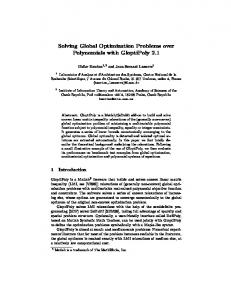
Figure 11: Network Flow of the sym-gcc of Example 8.2 (left) and the Strongly Connected Components of the Residual Graph (right). Example 8.2 We consider the same domains as for Example 8.1. There are 4 colors hence 4 set variables S1 , S2 , S3 , S4 . Color 1 is present only in the first and second slab hence S 1 = S 1 = {1, 2}. Color 2 and 3 can only come in the two first slabs S 2 = S 3 = φ and S 2 = S 3 = {1, 2}. Color 4 can be present in every slab S 4 = φ and S 4 = {1, 2, 3}. The sym-gcc imposing that at most two colors are present in each slab is: sym-gcc([S1 , S2 , S3 , S4 ], [2, 1, 1, 1], [l1 = 0, . . . , l3 = 0], [u1 = 2, . . . , u3 = 2]). The corresponding network flow and a valid flow is depicted on Figure 11 (left). Each arc is annotated with the unit(s) of flow through this arc and the (demand,capacity). One can check that the flow is valid since the flow conservation as well as the demand and capacity requirements are satisfied. The residual network and the strongly connected components (scc’s) are represented on the right of Figure 11. Vertices belonging to the same strongly connected components are labeled with the same capital letter. Zero flow arcs are S4 → 1 and S4 → 2 and there is only one non zero arc with end-points in different SCCs (other than arcs with demand > 0) that is S4 → 3. Consequently, 3 is added to the lower bound of S4 , and 1 and 2 are removed from its upper bound which means that S4 is bound to {3}. Now, since S4 = {X5 }, it means that order o5 must be assigned to slab 3: Dom(X5 ) = {6 1, 6 2, 3}. This filtering was not possible in Example 8.1 without the sym-gcc.

8.4

Experimental Results

In our first experiment, we compare the CP model with and without the sym-gcc to minimize the number of slabs by imposing a loss of 0 on the 100 instances

20

600 500

CP−DSB−VAL without sym−gcc CP−DSB−VAL with sym−gcc

100

200

time(s) 300

400

●

●

0

●

20

● ● ● ● ●

40

● ● ● ● ● ● ● ● ● ●● ●● ● ● ● ● ● ● ● ● ●

60 number of orders

80

100

Figure 12: Experimental Results of CP to Minimize the Number of Slabs on the CSPLib Instance With and Without the sym-gcc Constraint. derived from the single instance in CSPLib (remember that for all these instances there exists a solution with a loss of 0). To find the minimum number of slabs, we solve a series of satisfaction problems with increasing number of slabs. We start with the lower bound (color+bin-packing) on the number of slabs until a solution is found which is optimal by construction.7 The time-out is 500 seconds. The results of Figure 12 show that the sym-gcc allows us to solve optimally all the instances but one (with 33 slabs), while 69 instances could not be solved without this global constraint. The most difficult instances are exactly those for which the lower bound color+bin-packing (light gray line on Figure 10) is below the exact minimum number of slabs (black line on Figure 10). The time required by these instances are marked with a circle on Figure 12. For those instances, most of the time is spent to prove that there is no solution with the number of slabs found by the lower bound color+bin-packing. Finding the optimal solution is very easy (less than 1.5 seconds and 77 backtracks for all the instances). We can conclude from this first experiment that the difficulty of this problem is not to find an optimal solution but to prove its optimality. It is important however to remember that, without the sym-gcc, even finding an optimal solution is difficult for most of the instances. In our second experiment, we compare the CBLSs approach with the CP+ sym-gcc. The objective is to discover which technique is more appropriate to 7 This approach is classical when optimizing something on the structure of the problem as the number of bins in bin-packing [10].

21

35

CBLSs CP−DSB−VAL with sym−gcc

5

10

time (s) 15 20

25

30

●

● ●

0

● ●

●

●

●

20

●

●

●

●

●

●

●

40

●

●

●

●

●

●

●

●

●

60 number of orders

●

●

●

80

●

●

●

●

●

●

●

●

100

Figure 13: Time to Find the Optimal Solution with CP+sym-gcc and CBLSs when Minimizing the Number of Slabs on the CSPLib Instance. find good solutions quickly (without proving optimality). For this reason, we start from an upper bound on the number of slabs and, each time a solution is found, the next one is constrained to have fewer slabs. We compare the two approaches with the time necessary to find the best solution. The time is averaged on five runs on each instance for CBLSs . The results are given on Figure 13. It seems that CP-DSB+sym-gcc is faster than CBLSs on these instances and also more stable. Finally, we also made some experiments on 267 difficult instances from the 380 generated instances having a known solution with zero loss. On these instances, 99 could not be solved by CP-DSB-VAL, only 13 could not be solved by CBLSs , and 167 instances could be solved by both approaches. The total number of slabs used on instances that could be solved by both is 8206 for CP and 7897 for CBLSs . On these 184 instances, CP-DSB-VAL is never strictly better, while CBLSs is strictly better on 100 instances. These results might be contradictory with the results of Figure 13 but are not so surprising. Indeed, finding a solution with zero loss is already very difficult for CP-DSB-VAL when there are less than 18 capacities. Not surprisingly, minimizing the number of slabs by constraining the loss to be zero was not more successful. On such instances with less than 18 capacities, CBLSs should be preferred over pure CP. Since LNS was very good also when there is a few number of capacities (see Section 7) we investigate another approach to solve this problem using the LNS model of Section 5 + the sym-gcc constraint starting from an upper-bound on the number of slabs: 22

• If a solution with a zero loss is found with LNS within the timeout period, the number of slabs is constrained to be the number of slabs used -1 in this solution. The LNS process is repeated with this new number of slabs unless it is smaller than the lower bounds given on Section 8.1. • Else if at least one solution with zero loss was found during the process, the last solution found with a zero loss is reported as the best one. On the 267 difficult instances from the 380 generated instances having a known solution with zero loss, 29 could not be solved by LNS, only 13 could not be solved by CBLSs , and 233 instances could be solved by both approaches. The total number of slabs used on instances that could be solved by both is 11192 for LNS and 11009 for CBLSs . On these 184 instances, LNS is strictly better on 2 instances while CBLSs is strictly better on 110 instances. We can conclude that LNS obtains better results than pure CP but is still clearly behind CBLSs on the slabs minimization problem.

9

Conclusion

This paper evaluated CP, LNS, and CBLS approaches on the Steel Mill Slab Design problem, a well-known benchmark in the CP community. The approaches are all based on the same high-level model originally proposed by Garnani and Refalo. Since the traditional instance of the CSP library can be solved in 50ms by CBLS, the paper considered harder instances with fewer available capacities. The experimental results on these instances indicated that CBLS and LNS dominates the pure CP. Moreover, a CBLS approach maintaining feasibility typically outperforms a CBLS approach with soft constraints, except on instances with very few available slab capacities. The LNS approach obtains very competitive results in terms of quality of the objective but reaches the best solution less often than the CBLS model maintaining feasibility. The paper also considered a generalization of the problem in which the number of slabs must be minimized for a fixed loss. For this new problem, the paper proposed a CP approach using a global symmetric cardinality constraints and a CBLS approach exploring infeasible solutions. The experimental results demonstrated the benefits of the global constraint. They also indicated that CP is effective on this problem when many capacities are available, and that CBLS dominates CP and LNS when the number of capacities decreases.

References [1] Problem 38 of CSPLIB (www.csplib.org). [2] Comet 2.1. www.dynadec.com. [3] Antoine Gargani and Philippe Refalo. An efficient model and strategy for the steel mill slab design problem. In Christian Bessiere, editor, Principles 23

and Practice of Constraint Programming - CP 2007, 13th International Conference, volume 4741 of Lecture Notes in Computer Science, pages 77– 89. Springer, 2007. [4] Carmen Gervet. New structures of symbolic constraint objects: sets and graphs. In In 3rd Workshop on Constraint Logic Programming, Marseille, France, March, 1993. [5] Pascal Van Hentenryck and Laurent Michel. The steel mill slab design problem revisited. In Laurent Perron and Michael A. Trick, editors, Integration of AI and OR Techniques in Constraint Programming for Combinatorial Optimization Problems, 5th International Conference, CPAIOR 2008, volume 5015 of Lecture Notes in Computer Science, pages 377–381. Springer, 2008. [6] Waldemar Kocjan and Per Kreuger. Filtering methods for symmetric cardinality constraint. In Jean-Charles R´egin and Michel Rueher, editors, Integration of AI and OR Techniques in Constraint Programming for Combinatorial Optimization Problems, First International Conference, CPAIOR 2004, volume 3011 of Lecture Notes in Computer Science, pages 200–208. Springer, 2004. [7] Silvano Martello and Paolo Toth. Knapsack Problems: Algorithms and Computer Implementations. Wiley Interscience Series in Discrete Mathematics and Optimization. John Wiley & Sons Ltd., Baffins Lane, Chichester, West Sussex PO19 1UD, England, 1990. [8] Jean-Charles R´egin. Generalized arc consistency for global cardinality constraint. In AAAI ’94: Proceedings of the twelfth national conference on Artificial intelligence (vol. 1), pages 209–215. American Association for Artificial Intelligence, 1996. [9] Paul Shaw. Using constraint programming and local search methods to solve vehicle routing problems. In Michael J. Maher and Jean-Francois Puget, editors, Principles and Practice of Constraint Programming - CP98, 4th International Conference, volume 1520 of Lecture Notes in Computer Science, pages 417–431. Springer, 1998. [10] Paul Shaw. A constraint for bin packing. In Mark Wallace, editor, Principles and Practice of Constraint Programming - CP 2004, 10th International Conference, CP 2004, volume 3258 of LNCS, pages 648–662. Springer, 2004. [11] Pascal Van Hentenryck and Laurent Michel. Constraint-Based Local Search. MIT Press, 2005. [12] J. Walser. Solving linear pseudo-boolean constraints with local search. In Proceedings of the Eleventh Conference on Artificial Intelligence, pages 269–274, 1997.

24