May 10, 2007 - Manchester Institute for Mathematical Sciences ... The University of Manchester. Reports .... the code has to be vectorized in the SIMD sense, by.
Solving Systems of Linear Equations on the CELL Processor Using Cholesky Factorization Jakub Kurzak, Alfredo Buttari and Jack Dongarra July 2007
MIMS EPrint: 2007.95
Manchester Institute for Mathematical Sciences School of Mathematics The University of Manchester
Reports available from: And by contacting:
http://www.manchester.ac.uk/mims/eprints The MIMS Secretary School of Mathematics The University of Manchester Manchester, M13 9PL, UK
ISSN 1749-9097
Solving Systems of Linear Equations on the CELL Processor Using Cholesky Factorization – LAPACK Working Note 184 Jakub Kurzak1 , Alfredo Buttari1 , Jack Dongarra1,2 1
2
Department of Computer Science, University Tennessee, Knoxville, Tennessee 37996
Computer Science and Mathematics Division, Oak Ridge National Laboratory, Oak Ridge, Tennessee, 37831 May 10, 2007
1
ABSTRACT: The STI CELL processor introduces pioneering solutions in processor architecture. At the same time it presents new challenges for the development of numerical algorithms. One is effective exploitation of the differential between the speed of single and double precision arithmetic; the other is efficient parallelization between the short vector SIMD cores. In this work, the first challenge is addressed by utilizing a mixed-precision algorithm for the solution of a dense symmetric positive definite system of linear equations, which delivers double precision accuracy, while performing the bulk of the work in single precision. The second challenge is approached by introducing much finer granularity of parallelization than has been used for other architectures and using a lightweight decentralized synchronization. The implementation of the computationally intensive sections gets within 90 percent of peak floating point performance, while the implementation of the memory intensive sections reaches within 90 percent of peak memory bandwidth. On a single CELL processor, the algorithm achieves over 170 Gflop/s when solving a symmetric positive definite system of linear equation in single precision and over 150 Gflop/s when delivering the result in double precision accuracy. KEYWORDS: CELL BE, iterative refinement, mixed-precision algorithms, Cholesky factorization
Motivation
In numerical computing, there is a fundamental performance advantage of using single precision floating point data format over double precision data format, due to more compact representation, thanks to which, twice the number of single precision data elements can be stored at each stage of the memory hierarchy. Short vector SIMD processing provides yet more potential for performance gains from using single precision arithmetic over double precision. Since the goal is to process the entire vector in a single operation, the computation throughput can be doubled when the data representation is halved. Unfortunately, the accuracy of the solution is also halved. Most of the processor architectures available today have been at some point augmented with short vector SIMD extensions. Examples include Streaming SIMD Extensions (SSE) for the AMD and Intel lines of processors, PowerPC Velocity Engine / AltiVec / VMX, Sparc Visual Instruction Set (VIS), Alpha Motion Video Instructions (MVI), PA-RISC Multimedia Acceleration eXtensions (MAX), MIPS3D Application Specific Extensions (ASP), and Digital Media Extensions (MDMX), ARM NEON. The different architectures exhibit big differences in their capabilities. The vector size is either 64 bits or, more commonly, 128 bits. The register file size ranges from 1
order to improve the computed solution, an iterative refinement process can be applied, which produces a correction to the computed solution at each iteration. In principle, the algorithm can produce a solution correct to the working precision. Iterative refinement is a fairly well understood concept and was analyzed by Wilkinson [4], Moler [5] and Stewart [6]. Higham gives error bounds for both single and double precision iterative refinement algorithms, where the entire algorithm is implemented with the same precision (single or double respectively) [7]. He also gives error bounds in single precision arithmetic, with refinement performed in double precision arithmetic. Error analysis for the case described in this work, where the factorization is performed in single precision and the refinement in double precision, is given by Langou et al. [8]. The authors of this work have previously presented an initial implementation of the mixed-precision algorithm for the general, non-symmetric, case using LU factorization on the CELL processors. Although respectable performance numbers were presented, both the factorization and the refinement steps relied on rather classic parallelization approaches. Also, a somewhat general discussion of algorithmic and implementation details was presented. This work extends the previous presentation by introducing a novel scheme for parallelization of the computational components of the algorithm, and also describes in much more detail the implementation of both computation-intensive, as well as memory-intensive operations.
just a few to as many as 128 registers. Some extensions only support integer types, others also operate on single precision floating point numbers, and yet others also process double precision values. Today the Synergistic Processing Element (SPE) of the STI CELL processor [1–3] can probably be considered the state of the art in short vector SIMD processing. Possessing 128-byte long registers and a fully pipelined, fused add-multiply instruction, it is capable of completing eight single precision floating point operations each clock cycle, which combined with the size of the register file of 128 registers delivers close to peak performance on many common workloads. At the same time, built with multimedia and embedded applications in mind, the current incarnation of the CELL architecture does not implement double precision arithmetic on par with single precision performance, which makes the processor a very attractive target for exploring mixed-precision approaches. Another important phenomenon in recent years has been the gradual shift of focus in processor architecture from aggressive exploitation of instruction level parallelism towards thread-level parallelism, resulting in the introduction of chips with multiple processing units commonly referred to as multi-core processors. The new architectures deliver the much desired improvement in performance, and at the same time challenge the scalability of existing algorithms, and force the programmers to seek more parallelism by going to much finer levels of problem granularity. In linear algebra, it enforces the departure from the model relying on parallelism encapsulated at the level of BLAS and shifts to more flexible methods of scheduling work.
2
3
Algorithm
The standard approach to solving symmetric positive definite systems of linear equations is to use the Cholesky factorization. The Cholesky factorization of a real symmetric positive definite matrix A has the form A = LLT , where L is a real lower triangular matrix with positive diagonal elements. The system is solved by first solving Ly = b (forward substitution) and then solving LT x = y (backward substitution). In order to improve the accuracy of the computed solution, an iterative refinement process is applied, which
Related Work
Iterative refinement is a well known method for improving the solution of a linear system of equations of the form Ax = b. Typically, a dense system of linear equations is solved by applying a factorization to the coefficient matrix, followed by a back solve. Due to roundoff errors, the solution carries an error related to the condition number of the coefficient matrix. In 2
Algorithm 1 Solution of a symmetric positive defiThe algorithm described above, and shown on Alnite system of linear equations using mixed-precision gorithm 1 is available in the LAPACK 3.1 library and iterative refinement based on Cholesky factorization. implemented by the routine DSGESV. 1: A(32) , b(32) ← A, b a 2: L(32) , LT (32) ←SPOTRF (A(32) ) 3:
4
(1)
x(32) ←SPOTRSb (L(32) , LT(32) , b(32) ) (1)
x(1) ← x(32) 5: repeat 6: r(i) ← b − Ax(i) (i) 7: r(32) ← r(i)
4:
(i)
4.1
z(32) ←SPOTRSb (L(32) , LT(32) , r(32) )
9:
z (i) ← z(32)
10: 11:
Essential Hardware Features
An extensive hardware overview would be beyond the scope of this publication. Vast amounts of information are publicly available for both experienced programmers [9], as well as newcomers to the field [10, 11]. It is assumed that the reader has some familiarity with the architecture. Here, the features are mentioned that have the most influence on the implementation presented. The CELL is a multi-core chip that includes nine different processing elements. One core, the POWER Processing Element (PPE), represents a standard processor design implementing the PowerPC instruction set. The remaining eight cores, the Synergistic Processing Elements (SPEs), are short vector Single Instruction Multiple Data (SIMD) engines with big register files of 128 128-bit vector registers and 256 KB of local memory, referred to as local store (LS). Although standard C code can be compiled for the execution on the SPEs, the SPEs do not execute scalar code efficiently. For efficient execution, the code has to be vectorized in the SIMD sense, by using C language vector extensions (intrinsics), or by using assembly code. The system’s main memory is accessible to the PPE through L1 and L2 caches and to the SPEs through DMA engines associated with them. The SPEs can only execute code residing in the local store and can only operate on data in the local store. All data has to be transferred in and out of local store via DMA transfers. The theoretical computing power of a single SPE is 25.6 Gflop/s in single precision and roughly 1.8 Gflop/s in double precision. Floating point arithmetic follows the IEEE format, with double precision operations complying numerically with the standard and single precision providing only rounding toward zero. The theoretical communication speed for a sin-
(i)
8:
Implementation
(i)
x(i+1) ← x(i) + z (i) until x(i) is accurate enough a LAPACK
name for Cholesky factorization name for symmetric back solve 64-bit representation is used in all cases where 32-bit representation is not indicated by a subscript. b LAPACK
produces a correction to the computed solution, x. The mixed-precision iterative refinement algorithm using Cholesky factorization is outlined by Algorithm 1. The factorization A = LLT (line 2) and the solution of the triangular systems Ly = b and LT x = y (lines 3 and 8) are computed using single precision arithmetic. The residual calculation (line 6) and the update of the solution (line 10) are computed using double precision arithmetic and the original double precision coefficients. The most computationally expensive operations, including the factorization of the coefficient matrix A and the forward and backward substitution, are performed using single precision arithmetic and they take advantage of the single precision speed. The only operations executed in double precision are the residual calculation and the update of the solution. It can be observed that all operations of O(n3 ) complexity are handled in single precision, and all operations performed in double precision are of at most O(n2 ) complexity. The coefficient matrix A is converted to single precision for the LU factorization. At the same time, the original matrix in double precision is preserved for the residual calculation. 3
T = T – A AT SSYRK
A
T
T = LLT SPOTRF
C = C – B AT SGEMM
T
A B
A
T
T
T C
A B
C=C\T STRSM
C
T C
C
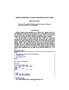
Figure 1: Top - steps of left-looking Cholesky factorization. Bottom - tiling of operations. the Cholesky factorization, which follows the implementation of the LAPACK routine SPOTRF. Due to the limited size of the local store, all numerical operations have to be decomposed into elementary operations that fit in the local store. The simplicity of implementing the Cholesky factorization lies in the fact that it can be easily decomposed into tile operations - operations on fixed-size submatrices that take from one to three tiles as input and produce one tile 4.2 Factorization as output. These elementary operations will further A few varieties of Cholesky factorization are known. be referred to as tile kernels. Figure 1 illustrates the In particular, the right-looking variant and the steps of the left-looking Cholesky factorization and left-looking variant [12]. It has also been pointed out how each step is broken down to tile operations. that those variants are borders of a continuous spectrum of possible execution paths [13]. 4.2.1 Computational Kernels Generally, the left-looking factorization is preferred for several reasons. During the factorization, most Implementation of the tile kernels assumes a fixed time is spent calculating a matrix-matrix product. In size of the tiles. Smaller tiles (finer granularity) have the case of the right-looking factorization, this prod- a positive effect on scheduling for parallel execution uct involves a triangular matrix. In the case of the and facilitate better load balance and higher parallel left-looking factorization, this product only involves efficiency. Bigger tiles provide better performance in rectangular matrices. It is generally more efficient sequential execution on a single SPE. In the case of the CELL chip, the crossover point to implement a matrix-matrix product for rectangular matrices and it is easier to balance the load is rather simple to find for problems in dense linear in parallel execution. The implementation presented algebra. From the standpoint of this work, the most here is derived from the left-looking formulation of important operation is matrix multiplication in single SPE is 25.6 GB/s. The theoretical peak bandwidth of the main memory is 25.6 GB/s as well. The size of the register file and the size of the local store dictate the size of the elementary operation subject to scheduling to the SPEs. The ratio of computing power to the memory bandwidth dictates the overall problem decomposition for parallel execution.
4
Operation
mizing the matrix multiplication (SGEMM1 ) kernel performing the calculation C = C − B × AT , since this operation dominates the execution time. All the tile kernels were written by consistently applying the idea of blocking with a block size of four. A short discussion of each case follows. The SSYRK kernel applies a symmetric rank-k update to a tile. In other words, it performs the operation T ← T − A × AT , where only the lower triangular part of T is modified. The SSYRK kernel consists of two nested loops, where in each inner iteration a 4×4 block of the output tile is produced and the body of the inner loop is completely unrolled. The #define and nested #define directives are used to create a single basic block - a block of straight line code. Static offsets are used within the basic block, and pointer arithmetic is used to advance pointers between iterations.
BLAS / LAPACK Call
T ← T − A × AT C ← C − B × AT B ← B × T −T T a
(B = B/T )
T ← L × LT
cblas ssyrk(CblasRowMajor, CblasLower, CblasNoTrans, 64, 64, 1.0, A, 64, 1.0, T, 64); cblas sgemm(CblasRowMajor, CblasNoTrans, CblasTrans, 64, 64, 64, 1.0, B, 64, A, 64, 1.0, C, 64); cblas strsm(CblasRowMajor, CblasRight, CblasLower, CblasTrans, CblasNonUnit, 64, 64, 1.0, T, 64, B, 64); lapack spotrf(lapack lower, 64, trans(T), 64, &info);b
a using
MATLAB notation
b using
LAPACK C interface by R. Delmas and J. Langou,
http://icl.cs.utk.edu/∼delmas/lapwrapc.html
Table 1: Single precision Cholesky tile kernels. gle precision. It turns out that this operation can achieve within a few percent off the peak performance on a single SPE for matrices of size 64×64. The fact that the peak performance can be achieved for a tile of such a small size has to be attributed to the large size of the register file and fast access to the local store, undisturbed with any intermediate levels of memory. Also, such a matrix occupies a 16 KB block of memory, which is the maximum size of a single DMA transfer. Eight such matrices fit in half of the local store providing enough flexibility for multibuffering and, at the same time, leaving enough room for the code. Discussion of tile size consideration was also presented before by the authors of this publication [14]. Table 1 represents the Cholesky tile kernels for tile size of 64×64 as BLAS and LAPACK calls. It has already been pointed out that a few derivations of the Cholesky factorization are known, in particular the right-looking variant and the left-looking variant [12]. Dynamic scheduling of operations is another possibility. However, no matter which static variant is used, or whether dynamic execution is used, the same set of tile kernels is needed. The change from one to another will only alter the order in which the tile operations execute. All the kernels were developed using SIMD C language extensions. Extra effort was invested into opti-
Algorithm 2 SSYRK tile kernel T ← T − A × AT . 1: for j = 0 to 15 do 2: for i = 0 to j − 1 do 3: Compute block [j,i] 4: Permute/reduce block [j,i] 5: end for 6: Compute block [j,j] 7: Permute/reduce block [j,j] 8: end for block is a 4×4 submatrix of tile T .
The construction of the SSYRK tile kernel is presented by Algorithm 2. The unrolled code consists of four distinct segments. A computation segment (line 3) includes only multiply and add operations to calculate a product of two 4×64 blocks of tile A and it produces 16 4-element vectors as output. A permutation/reduction segment (line 4) performs transpositions and reductions on these 16 vectors and delivers the four 4-element vectors constituting the 4×4 block of the output tile. The two segments mentioned above handle the off-diagonal, square blocks (lines 3 and 4), and two more segments handle the triangular, 1 Tile kernels are referred to using the names of BLAS and LAPACK routines implementing the same functionality.
5
Algorithm 3 SGEMM tile kernel C ← C − B × AT 1: Compute block 0 2: for i = 1 to 127 do 3: Permute/reduce blk 2i−2 & compute blk 2i−1 4: Permute/reduce blk 2i − 1 & compute blk 2i 5: end for 6: Permute/reduce blk 254 & compute blk 255 7: Permute/reduce blk 255
The STRSM kernel computes a triangular solve with multiple right-hand-sides B ← B × T −T . The computation is conceptually easiest to SIMD’ize if the same step is applied at the same time to different right-hand-sides. This can be easily achieved if the memory layout of tile B is such that each 4-element vector contains elements of the same index of different right-hand-sides. Since this is not the case here, each 4×4 block of the tile is transposed, in place, before and after the main loop implementing the solve. The operation introduces a minor overhead, but allows for a very efficient implementation of the solve one which achieves good ratio of the peak with small and simple code. Algorithm 4 presents the structure of the code implementing the triangular solve, which is an application of the lazy variant of the algorithm. The choice of the lazy algorithm versus the aggressive algorithm is arbitrary. The code includes two segments of fully unrolled code, both of which operate on 64×4 blocks of data. The outer loop segment (line 5) produces a 64×4 block j of the solution. The inner loop segment (line 3) applies the update of step i to block j.
blk is a 4×4 submatrix of tile C.
diagonal blocks (lines 6 and 7). It is an elegant and compact, but suboptimal design. The SGEMM kernel performs the operation C ← C − B × AT , which is very similar to the operation performed by the SSYRK kernel. One difference is that it updates the tile C with a product of two tiles, B and AT , and not the tile A and its transpose. The second difference is that the output is the entire tile and not just its lower triangular portion. Also, since the SGEMM kernel is performance-critical, it is subject to more optimizations compared to the SSYK kernel. The main idea behind additional optimization of Algorithm 5 SPOTRF tile kernel T ← L × LT . the SGEMM kernel comes from the fact that the SPE 1: for k = 0 to 15 do is a dual issue architecture, where arithmetic opera2: for i = 0 to k − 1 do tions can execute in parallel with permutations of 3: SSYRK (apply block [k,i] to block [k,k]) vector elements. Thanks to this fact, a pipelined ex4: end for ecution can be implemented, where the operations of 5: SPOTF2 (factorize block [k,k]) the permute/reduce segment from iteration k can be 6: for j = k to 15 do mixed with the operations of the compute segment 7: for i = 0 to k − 1 do from iteration k + 1. The two nested loops used for 8: SGEMM (apply block [j,i] to block [j,k]) SSYRK are replaced with a single loop, where the 9: end for 256 4×4 blocks of the output tile are produced in a 10: end for linear row-major order, which results in Algorithm 3. 11: for j = k to 15 do 12: STRSM (apply block [k,k] to block [j,k]) Algorithm 4 STRSM tile kernel B ← B × T −T . 13: end for 1: for j = 0 to 15 do 14: end for 2: for i = 0 to j − 1 do block is a 4×4 submatrix of tile T . 3: Apply block i towards block j 4: end for The SPOTRF kernel computes the Cholesky fac5: Solve block j torization, T ← L × LT , of a 64×64 tile. This is 6: end for the lazy variant of the algorithm, more commonly reblock is a 64×4 submatrix of tile B. ferred to as the left-looking factorization, where up6
Kernel Kernel SSYRK SGEMM STRSM SPOTRF a version b version
Source Code [LOC] 160 330 310 340
Compilation
spuxlca -O3 spu-gccb -Os spuxlca -O3 spu-gccb -O3
Object Code [KB] 4.7 9.0 8.2 4.1
Execution Time [µs] 13.23 22.78 16.47 15.16
Execution Rate [Gflop/s] 20.12 23.01 15.91 5.84
Fraction of Peak [%] 78 90 62 23
1.0 (SDK 1.1) 4.0.2 (toolchain 3.2 - SDK 1.1)
Table 2: Performance of single precision Cholesky factorization tile kernels. dates to the trailing submatrix do not immediately pecially register file and memory organization. It is worth noting that, although significant effort follow panel factorization. Instead, updates are applied to a panel right before factorization of that was required to optimize the SGEMM kernel (and yet more would be required to further optimize it), panel. It could be expected that this kernel is imple- the other kernels involved a rather small programmented using Level 2 BLAS operations, as this is the ming effort in a higher level language to deliver satusual way of implementing panel factorizations. Such isfactory performance (execution time shorter than a solution would, however, lead to code being diffi- execution time of SGEMM kernel). This means that cult to SIMD’ize and yield very poor performance. the Pareto principle (also known as the 80-20 rule) Instead, the implementation of this routine is simply (http://en.wikipedia.org/wiki/Pareto principle) apan application of the idea of blocking with block size plies very well in this case. Only a small portion equal to the SIMD vector size of four. Algorithm 5 of the code requires strenuous optimizations for the application to deliver close to peak performance. presents the structure of the SPOTRF tile kernel. Table 2 compares the tile kernels in terms of source and object code size and performance. Although performance is the most important metric, code size is not without meaning, due to the limited size of local store. Despite the fact that code can be replaced in the local store at runtime, it is desirable that the entire code that implements the single precision factorization fits into the local store at the same time. Code motion during the factorization would both complicate the code and adversely affect performance.
4.2.2
Parallelization
The presentation of the parallelization of the Cholesky factorization needs to be preceded by a discussion of memory bandwidth considerations. The SGEMM kernel can potentially execute at a rate very close to 25.6 Gflop/s on a single SPE. In such a case, it performs the 2 × 643 = 524288 operations in 20.48 µs. The operation requires the transmission of three tiles from main memory to the local Although the matrix multiplication achieves quite store (tiles A, B and C) and a transmission of one good performance - 23 Gflop/s, which is 90 percent of tile from local store to main memory (updated tile the peak, there is no doubt that better performance C), consuming the bandwidth equal to: could be achieved by using assembly code instead 4tiles × 642 × 4sizeof (f loat) [B] C language SIMD extensions. Performance in excess = 3.2[GB/s]. 20.48[µs] of 25 Gflop/s has been reported for similar, although not identical, SGEMM kernels [15]. It is remarkable This means that eight SPEs performing the SGEMM that this performance can be achieved for operations operation at the same time will require the bandof such small granularity, which has to be attributed width of 8 × 3.2GB/s = 25.6GB/s, which is the theto the unique features of the CELL architecture, es- oretical peak main memory bandwidth. 7
It has been shown that arithmetic can execute almost at the theoretical peak rate on the SPE. At the same time, it would not be realistic to expect theoretical peak bandwidth from the memory system. By the same token, data reuse has to be introduced into the algorithm to decrease the load on the main memory. A straightforward solution is to introduce 1D processing, where each SPE processes one row of tiles of the coefficient matrix at a time. Please see Figure 1 for the following discussion. In the SSYRK part, one SPE applies a row of tiles A to the diagonal tile T , followed by the SPOTRF operation (factorization) of the tile T . Tile T only needs to be read in at the beginning of this step and written back at the end. The only transfers taking place in between are reads of tiles A. Similarly, in the SGEMM part, one SPE applies a row of tiles A and a row of tiles B to tile C, followed by the STRSM operation (triangular solve) on tile C using the diagonal, triangular tile T . Tile C only needs to be read in at the beginning of this step and written back at the end. Tile T only needs to be read in right before the triangular solve. The only transfers taking place in between are reads of tiles A and B. Such work partitioning approximately halves the load on the memory system. It may also be noted that 1D processing is a natural match for the left-looking factorization. In the right-looking factorization, the update to the trailing submatrix can easily be partitioned in two dimensions. However, in case of the left-looking factorization, 2D partitioning would not be feasible due to the write dependency on the panel blocks (tiles T and C). 1D partitioning introduces a load balancing problem. With work being distributed by block rows, in each step of the factorization, a number of processors is going to be idle, which is equal to the number of block rows factorized in a particular step modulo the number of processors. Figure 2 shows three consecutive steps on a factorization with the processors being occupied and idle in these steps. Such behavior is going to put a harsh upper bound on achievable performance. It can be observed, however, that at each step of the factorization, a substantial amount of work can be scheduled, to the otherwise idle processors, from
1 2
1
3
2
4
3
2
5
4
3
6
5
4
7
6
5
8
7
6
8
7
1
8
Figure 2: Load imbalance caused by 1D processing. the upcoming steps of the factorization. The only operations that cannot be scheduled at a given point in time are those that involve panels that have not been factorized yet. This situation is illustrated in Figure 3. Of course, this kind of processing requires dependency tracking in two dimensions, but since all operations proceed at the granularity of tiles, this does not pose a problem.
1 2
5
3
6
8
4
7
...
Figure 3: Pipelining of factorization steps. In the implementation presented here, all SPEs follow a static schedule presented in Figure 3, with cyclic distribution of work from the steps of the factorization. In this case, a static schedule works well, due to the fact that performance of the SPEs is very deterministic (unaffected by any non-deterministic phenomena, like cache misses). This way the potential bottleneck of a centralized scheduling mechanism is avoided. Figure 4 presents the execution chart (Gantt chart) of factorization of a 1024×1024 matrix. Colors correspond to the ones in Figure 1. The two shades 8
Figure 4: Execution chart of Cholesky factorization of a matrix of size 1024×1024. Color scheme follows the one from Figure 1. Different shades of green correspond to odd and even steps of the factorization. of green distinguish the SGEMM operation in odd and even steps of the factorization. The yellow color marks the barrier operation, which corresponds to the load imbalance of the algorithm. It can be observed that; load imbalance is minimal (the yellow region), dependency stalls are minimal (the white gaps), and communication and computation overlapping is very good (the colored blocks represent purely computational blocks).
table. The SPE completing the factorization of a tile updates the progress tables of all other SPEs, which is done by a DMA transfer and which introduces no overhead due to the non-blocking nature of these transfers. Since the smallest amount of data subject to DMA transfer is one byte, the progress table entries are one byte in size. These transfers consume an insignificant amount of bandwidth of the EIB and their latency is irrelevant to the algorithm.
4.2.3
4.2.4
Synchronization
Communication
The most important feature of communication is double-buffering of data. With eight tile buffers available, each operation involved in the factorization can be double-buffered independently. Thanks to this fact, double-buffering is implemented not only between operations of the same type, but also between different operations. In other words data is always prefetched for the upcoming operation, no matter what operation it is. In absence of dependency stalls, the SPEs never wait for data, which results in big portions of the execution chart without any gaps between computational blocks (Figure 5). Tiles are never exchanged internally between local stores, but always read from main memory and written to main memory. An attempt to do otherwise could tie up buffers in the local store and prevent asynchronous operation of SPEs. At the same time, with the work partitioning implemented here, the memory system provides enough bandwidth to fully overlap communication and computation. Reads of tiles involve dependency checks. When it comes to prefetching of a tile, a dependency is tested and a DMA transfer is initiated if the dependency is satisfied. The DMA completion is tested right before
With the SPEs following a static schedule, synchronization is required, such that an SPE does not proceed if data dependencies for an operation are not satisfied. Several dependencies have to be tracked. The SSYRK and SGEMM operations cannot use as input tiles A and B that have not been factorized yet. The off-diagonal tiles A and B are factorized if the STRSM operation has completed on these tiles. In turn the STRSM operation cannot use as input a diagonal tile T that has not been factorized yet. A diagonal tile T is factorized if the SPOTRF operation has completed on this tile. Dependency tracking is implemented by means of a replicated progress table. The progress table is a 2D triangular array with each entry representing a tile of the coefficient matrix and specifies if the tile has been factorized or not, which means completion of a SPOTRF operation for diagonal tiles and STRSM operation for off-diagonal tiles. By replication of the progress table, the potential bottleneck of a centralized progress tracking mechanism is avoided. Each SPE can check dependencies by testing an entry in its local copy of the progress 9
Gflop/s
200
SP peak
175
SGEMM peak
150
SPOTRF
125 100 75 50 25 0
DP peak
0
1000
Figure 5: Magnification of a portion of the execution chart from Figure 4.
3000
4000
Figure 6: Performance of single precision Cholesky factorization.
processing of the tile. If the dependency is not satisfied in time for the prefetch, the prefetch is abandoned in order to not stall the execution. Instead, right before processing of the tile, the SPE busy-waits for the dependency and then transfers the tile in a blocking way (initiates the transfer and immediately waits for its completion). 4.2.5
2000
Size
Performance
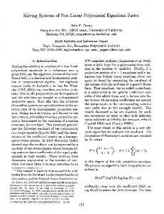
Figure 6 shows performance of the single precision Cholesky factorization calculated as the ratio of execution time to the number of floating point operations calculated as N 3 /3, where N is the matrix size of the input matrix. Table 3 gives numerical performance values for selected matrix sizes in Gflop/s and also as ratios relative to the peak of the processor of 204.8 Gflop/s and the peak of the SGEMM kernel of 8 × 23.01 = 184.8 Gflop/s. The factorization achieves 95 percent of the peak of the SGEMM kernel, which means that overheads of data communication, synchronization and load imbalance are minimal, and at this point the only inefficiency comes from the suboptimal performance of the SGEMM kernel. Hopefully in the future the kernel will be fully optimized, perhaps using hand-coded assembly. 10
Size 512 640 1024 1280 1536 1664 2176 4096
Gflop/s 92 113 151 160 165 166 170 175
% CELL Peak 45 55 74 78 80 81 83 85
% SGEMM Peak 50 62 82 87 89 90 92 95
Table 3: Selected performance points of single precision Cholesky factorization.
4.3
Refinement
The two most expensive operations of the refinement are the back solve (Algorithm 1, steps 3 and 8) and residual calculation (Algorithm 1, step 6). The back solve consists of two triangular solves involving the entire coefficient matrix and a single right-hand-side (BLAS STRSV operation). The residual calculation is a double precision matrix-vector product using a symmetric matrix (BLAS DSYMV operation). Both operations are BLAS Level 2 operations and on most processors would be strictly memory-bound.
The STRSV operation actually is a perfect example of a strictly-memory bound operation on the CELL processor. However, the DSYMV operation is on the border line of being memory bound versus compute bound due to very high speed of the memory system versus the relatively low performance of double precision arithmetic. 4.3.1
Triangular Solve
The triangular solve is a perfect example of a memory-bound workload, where the memory access rate sets the upper limit on achievable performance. The STRSV performs approximately two floating point operations per each data element of four bytes, which means that the peak memory bandwidth of 25.6 Gflop/s allows for at most
tiles. Triangular solve is performed on the diagonal tiles and a matrix-vector product (SGEMV equivalent) is performed on the off-diagonal tiles. Processing of the diagonal tiles constitutes the critical path in the algorithm. One SPE is solely devoted to processing of the diagonal tiles, while the goal of the others is to saturate the memory system with processing of the off-diagonal tiles. The number of SPEs used to process the off-diagonal tiles is a function of a few parameters. The efficiency of the computational kernels used is one of the factors. In this case, number four turned out to deliver the best results, with one SPE pursuing the critical path and three others fulfilling the task of memory saturation. Figure 7 presents the distribution of work in the triangular solve routines. x
25.6 GB/s × 2ops/f loat /4bytes/f loat = 12.8 Gf lop/s,
0
which is only 1/16 or 0.625 percent of the single precision floating point peak of the processor. Owing to this fact, the goal of implementing memory-bound operations is to get close to the peak memory bandwidth, unlike for compute-bound operations, where the goal is to get close to the floating point peak. This task should be readily achievable, given that a single SPE possesses as much bandwidth as the main memory. Practice shows, however, that a single SPE is not capable of generating enough traffic to fully exploit the bandwidth, and a few SPEs solving the problem in parallel should be used. Efficient parallel implementation of the STRSV operation has to pursue two goals: continuous generation of traffic in order to saturate the memory system and aggressive pursuit of the algorithmic critical path in order to avoid dependency stalls. A related question is the desired level of parallelism - optimal number of processing elements used. Since the triangular solve is rich in dependencies, increasing the number of SPEs increases the number of execution stalls caused by interprocessor dependencies. Obviously, there is a crossover point, a sweet spot, for the number of SPEs used for the operation. Same as other routines in the code, the STRSV operation processes the coefficient matrix by 64×64
A
1
0
2
2
3
3
1 2 3 1
1 0
2 0
3 0
1 0
0
2 0
3 0
1
11
Figure 7: Distribution of work in the triangular solve routine. The solve is done in place. The unknown/solution vector is read in its entirety by each SPE to its local store at the beginning and returned to the main memory at the end. As the computation proceeds, updated pieces of the vector are exchanged internally by means of direct, local store to local store, communication. At the end SPE 0 possesses the full solution vector and writes it back to the main memory. Synchronization is implemented analogously to the synchronization in the factorization and is based on the replicated triangular progress table (the same data structure is reused). Figure 8 shows performance, in terms of GB/s of the two triangular solve routines required in the solution/refinement step of the algorithm. The two rou-
lower portion is accessed, and implicit transposition is used to reflect the effect of the upper portion - each tile is read in only once, but applied to the output vector twice (with and without transposition). Since load balance is a very important aspect of the implementation, work is split among SPEs very evenly by applying the partitioning reflected in Figure 9. Such work distribution causes multiple write dependencies on the output vector and, in order to let each SPE proceed without stalls, the output vector is replicated on each SPE and the multiplication is followed by a reduction step. The reduction is also performed in parallel by all SPEs and introduces a very small overhead, compensated by the benefits of very good load balance.
Memory peak
24
20
GB/s
16
12
8
4
0
0
1000
2000
3000
4000
Size
x
Figure 8: Performance of the triangular solve routines.
0
tines perform slightly differently due to different performance of their computational kernels. The figure shows clearly that the goal of saturating the memory system is achieved quite well. Performance as high as 23.77 GB/s is obtained, which is 93 percent of the peak. 4.3.2
y
A
1
0
2
1
3
2
0
3
reduce 0
1
2
3
1 2 3
Figure 9: Distribution of work in the matrix-vector product routine.
Matrix-Vector Product
For most hardware platforms the matrix-vector product would be a memory-bound operation, the same as the triangular solve. On the CELL processor, however, due to the relative slowness of the double precision arithmetic, the operation is on the border of being memory-bound and compute-bound. Even with use of all eight SPEs, saturation of the memory is harder than in the case of the STRSV routine. The DSYMV routine also operates on tiles. Here, however, the double precision representation of the coefficient matrix is used with a tile size of 32×32, such that an entire tile can also be transferred with a single DMA request. The input vector is only read in once, at the beginning, in its entirety, and the output vector is written back after the computation is completed. Since the input matrix is symmetric, only the 12
Figure 10 shows the performance, in terms of GB/s, of the double precision, symmetric matrix-vector product routine. Performance of 20.93 GB/s is achieved, which is 82 percent of the peak. Although the DSYMV routine represents a Level 2 BLAS operation and is parallelized among all SPEs, it is still compute bound. Perhaps its computational components could be further optimized. Nevertheless, at this point the delivered level of performance is considered satisfactory
5
Limitations
The implementation presented here should be considered a proof of concept prototype with the pur-
Memory peak
24
200
SP peak
175
SGEMM peak
150
SPOTRF
20
Gflop/s
GB/s
16
12
SPOSV DSPOSV
125 100 75
8
50 4
0
25 0 0
1000
2000
3000
4000
Size
Figure 10: Performance of the matrix-vector product routine.
0
1000
2000
Size
3000
4000
Figure 11: Performance of the mixed-precision algorithm versus the single precision algorithm on IBM CELL blade system (using one CELL processor).
pose of establishing the upper bound on performance achievable for mixed-precision, dense linear algebra algorithms on the CELL processor. As such, it has a number of limitations. Only systems of that are multiples of 64 in size are accepted, and only systems with a single right hand side are supported. There are no tests for overflow during conversions from double to single precision. There is no test for non-definiteness during the single precision factorization step. The current implementation is wasteful in its use of the main memory. The entire coefficient matrix is stored explicitly without taking advantage of its symmetry, both in single precision representation and double precision representation. The maximum size of the coefficient matrix is set to 4096, which makes it possible to fit the progress table in each local store. this also makes it possible to fit the entire unknown/solution vector in each local store, which facilitates internal, local store to local store, communication and is very beneficial for performance.
6
DP peak
Results and Discussion
tem in single precision (SPOSV), and solution of the system in double precision by using factorization in single precision and iterative refinement to double precision (DSPOSV). These results were obtained on an IBM CELL blade using one of the two available CELL processors. Huge memory pages (16 MB) were used for improved performance. The performance is calculated as the ratio of the execution time to the number of floating point operations, set in all cases to N 3 /3. In all cases well conditioned input matrices were used, resulting in two steps of refinement delivering accuracy equal or higher than the one delivered by the purely double precision algorithm. At the maximum size of 4096, the factorization achieves 175 Gflop/s and the system solution runs at the relative speed of 171 Gflop/s. At the same time, the solution in double precision using the refinement technique delivers the relative performance of 156 Gflop/s, which is an overhead of less than 9 percent compared to the solution of the system in single precision. It can also be pointed out that by using the mixed-precision algorithm, double precision results are delivered at a speed over 10 times greater than the double precision peak of the processor.
Figure 11 compares the performance of a single precision factorization (SPOTRF), solution of the sys13
CELL processor is much lower than the single precision performance, mixed-precision algorithms permit exploiting the single precision speed while achieving full double precision accuracy.
160 SP peak
140 SGEMM peak
120
SPOTRF
SPOSV
Gflop/s
100
DSPOSV
8
80
One of the main considerations for the future is application of the pipelined processing techniques to factorizations where the panel does not easily split into independent operations, like the factorizations where pivoting is used. Another important question is the one of replacing the static scheduling of operations with dynamic scheduling by an automated system and also the impact of such mechanisms on programming ease and productivity.
60 40 20 0
DP peak
0
500
1000
1500
Future Plans
2000
Size
Figure 12: Performance of the mixed-precision algorithm versus the single precision algorithm on Sony PlayStation 3.
9
Acknowledgements
Figure 12 shows results obtained on the Sony PlayStation 3, using the six available SPEs and 256 KB1 available memory allocated using huge pages (16 MB). For the maximum problem size of 2048, the performance of 127 Gflop/s was achieved for the factorization, 122 Gflop/s for the single precision solution, and 104 Gflop/s for the double precision solution. In this case, the double precision solution comes at the cost of roughly 15 percent overhead compared to the single precision solution.
The authors thank Gary Rancourt and Kirk Jordan at IBM for taking care of our hardware needs and arranging for partial financial support for this work. The authors are thankful to numerous IBM researchers for generously sharing their CELL expertise, in particular Sidney Manning, Daniel Brokenshire, Mike Kistler, Gordon Fossum, Thomas Chen and Michael Perrone.
7
The code is publicly available at the location http://icl.cs.utk.edu/iter-ref/ → CELL BE Code.
Conclusions
The CELL Broadband Engine has a very high potential for dense linear algebra workloads offering a very high peak floating point performance and a capability to deliver performance close to the peak for quite small problems. The same applies to the memory system of the CELL processor, which allows for data transfer rates very close to the peak bandwidth for memory-intensive workloads. Although the double precision performance of the 1 only
approximately 200 KB available to the application
14
10
Code
References [1] H. P. Hofstee. Power efficient processor architecture and the Cell processor. In Proceedings of the 11th Int’l Symposium on High-Performance Computer Architecture, 2005. [2] J. A. Kahle, M. N. Day, H. P. Hofstee, C. R. Johns, T. R. Maeurer, and D. Shippy. Introduc-
tion to the Cell multiprocessor. IBM J. Res. & [14] J Kurzak and J. J. Dongarra. Implementation of mixed precision in solving systems of linear Dev., 49(4/5):589–604, 2005. equations on the CELL processor. Concurrency [3] IBM. Cell Broadband Engine Architecture, VerComputat.: Pract. Exper, 2007. in press, DOI: sion 1.0, August 2005. 10.1002/cpe.1164. [4] J. H. Wilkinson. Rounding Errors in Algebraic Processes. Prentice-Hall, 1963.
[15] T. Chen, R. Raghavan, J. Dale, and E. Iwata. Cell Broadband Engine architecture and its first implementation, A performance view. http://www-128.ibm.com/ developerworks/ power/ library/ pa-cellperf/, November 2005.
[5] C. B. Moler. Iterative refinement in floating point. J. ACM, 14(2):316–321, 1967. [6] G. W. Stewart. Introduction to Matrix Computations. Academic Press, 1973. [7] N. J. Higham. Accuracy and Stability of Numerical Algorithms. SIAM, 1996. [8] J. Langou, J. Langou, P. Luszczek, J. Kurzak, A. Buttari, and J. J. Dongarraa. Exploiting the performance of 32 bit floating point arithmetic in obtaining 64 bit accuracy. In Proceedings of the 2006 ACM/IEEE Conference on Supercomputing, 2006. [9] IBM. Cell Broadband Engine Programming Handbook, Version 1.0, April 2006. [10] IBM. Cell Broadband Engine Programming Tutorial, Version 2.0, December 2006. [11] A. Buttari, P. Luszczek, J. Kurzak, J. J. Dongarra, and G. Bosilca. A rough guide to scientific computing on the PlayStation 3, version 1.0. Technical Report UT-CS-07-595, Computer Science Department, University of Tennessee, 2007. http://www.cs.utk.edu/ library/ TechReports/ 2007/ ut-cs-07-595.pdf. [12] J. J. Dongarra, I. S. Duff, D. C. Sorensen, and H. A. van der Vorst. Numerical Linear Algebra for High-Performance Computers. SIAM, 1998. [13] J. Kurzak and J. J. Dongarraa. Implementing linear algebra routines on multi-core processors with pipelining and a look-ahead. In Proceedings of the 2006 Workshop on State-of-the-Art in Scientific and Parallel Computing (PARA’O6), Umea, Sweden, 2006. Lecture Notes in Computer Science series, Springer, 2007 (to appear). 15