2006) calls for a program that can determine the relationships between com- mon Hilbert-style axiomatizations of the modal logics K, T, S1, S1â¦, S3, S4 ...... ing with Analytic Tableaux and Related Methods, International Conference.
Solving the $100 Modal Logic Challenge Florian Rabe a,1 Petr Pudl´ak b,2 Geoff Sutcliffe c Weina Shen c a Department
of Computer Science, Carnegie Mellon University, USA
b Department
of Theoretical Computer Science and Mathematical Logic Charles University, Czech Republic
c Department
of Computer Science, University of Miami, USA
Abstract We present the theoretical foundation, design and implementation of a system that automatically determines the subset relation between two given axiomatizations of propositional modal logics. This is an open problem for automated theorem proving. Our system solves all but six out of 121 instances formed from 11 common axiomatizations of seven modal logics. Thus, although the problem is undecidable in general, our approach is empirically successful in practically relevant situations. Key words: Modal Logic, $100 challenge, subset relationship
1
Introduction and Related Work
Modal logics are extensions of classical logic that handle the concept of modalities. Modern modal logic was founded by Clarence Irving Lewis in his 1910 Harvard thesis, and further developed in a series of scholarly articles beginning in 1912. In his book Symbolic Logic (with C. H. Langford), he introduced the five well-known modal logics S1 through S5 (Lewis and Langford, 1932). The contemporary era in modal logic began in 1959 when Saul Kripke introduced semantics for modal logics (Kripke, 1963). The mathematical structures of modal logics are modal algebras – Boolean algebras augmented with unary operations. Their study began to emerge with McKinsey’s proof that S2 and S4 are decidable (McKinsey, 1941). Today plain propositional modal logic 1
The author was supported by a fellowship for Ph.D. research of the German Academic Exchange Service. 2 The author was supported by the Grant Agency of Charles University (grant no. 377/2005/A INF).
is standard knowledge, see, e.g., Hughes and Cresswell (1996), and first order modal logic has been thoroughly studied, e.g., Fitting and Mendelsohn (1998). Henceforth in this paper attention is limited to propositional modal logic with the standard modalities possibility and necessity. Many modal logics have multiple axiomatizations that are equivalent, in the sense that they generate the same theory - the same set of theorems. Similarly, one modal logic may be stronger than another in the sense that the stronger logic’s theory is a strict superset of that of the weaker logic. Finally, two modal logic may be incomparable with one another, because each has theorems that the other does not. Such relationships between different axiomatizations of individual modal logics and between different modal logics, are well known (Hughes and Cresswell, 1996). The Modal Logic $100 Challenge (Sutcliffe, 2006) calls for a program that can determine the relationships between common Hilbert-style axiomatizations of the modal logics K, T, S1, S1◦ , S3, S4 and S5 (see Halleck (2006) for an overview and a list of references to various modal logics and axiomatizations). The challenge was sponsored by John Halleck, who has a practical need for such a program as an aid to maintaining his overview (Halleck, 2006). Determining the relationship between two axiomatizations is undecidable in general (Blackburn et al., 2001). Decidability can be established separately for some modal logics. Historically, finding a complete Kripke semantics (Kripke, 1963) and establishing the finite model property by filtration (Lemmon, 1966) were used to obtain decidability of theoremhood. However, checking the subset relation between modal logics also involves checking the admissibility of rules. Here, decidability has been shown for a few cases, including K4 and S4 (Rybakov, 1997). Recently a framework has been developed in which admissibility is reduced to terminating analytic proofs for a variety of modal logics (Iemhoff and Metcalfe, 2007). In (Kracht, 1990) splittings are used to decide the admissibility of a rule for some logics, which correspond to transitive Kripke frames, but no algorithm is known for obtaining a splitting for an arbitrary logic. None of these methods is applicable to the full range of differently axiomatized modal logics. So far sophisticated implementations have focused on deriving theoremhood. (Gor´e et al., 1997) describe the Logics Work Bench program that is capable of reasoning about the modal systems K, KT, KT4, KT45 and KW. (Giunchiglia et al., 2002) use a SAT solver to decide a few classical systems. (Schmidt and Hustadt, 2006) give an overview over various methods based on translations of modal logic into first-order logic (e.g. Ohlbach and Schmidt, 1997). (Hustadt and Schmidt, 2000) extends the firstorder theorem prover SPASS with the ability to apply such translations to its input. This paper describes an implemented and tested system within which relationships between modal logics can be determined. The system has been applied
p, q, . . .
a countably infinite set of propositional variables
¬F
negation
(primitive)
∧F G
conjunction
(primitive)
3F
possibility
(primitive)
∨F G
disjunction
=def n ¬∧¬F ¬G
→FG
implication
=def n ¬∧F ¬G
↔FG
equivalence
=def n ∧→ F G → GF
⇒FG
strict implication
=def n 2 → F G
⇔FG
strict equivalence
=def n ∧ ⇒ F G ⇒ GF
2F
necessity
=def n ¬3¬F
Fig. 1. Atomic formulae and connectives
successfully to the $100 challenge. A partial preliminary version of this work has been presented as (Rabe, 2006b). The core idea is to use a simple translation to first-order logic (described in Section 3 of (Schmidt and Hustadt, 2006)), which encodes modal logic formulae as first-order terms, modal logic axioms and theorems as first-order atoms, and modal logic rules as first-order implications. This translation comes at the price of efficiency (McCune and Wos, 1992). We use it because it is applicable to any modal logic, in particular non-normal logics. Since we do not presuppose any semantics, the applicability of any other translation would itself have to be established automatically (which we do in the Kripke-based strategy described in Section 3.4). With this encoding, reasoning is performed using several modularly implemented (possibly incomplete) strategies, using first-order automated reasoning tools to prove or disprove the subset relationship: direct strategies, strategies based on Kripke semantics, and algebraic strategies that represent modal logics as modal algebras.
Section 2 provides the necessary background in modal logic and the encoding in first-order logic. Section 3 describes the implementation of our system and the theoretical basis and implementation of the strategies. Section 4 documents and analyzes the results achieved by the system in attacking the $100 Challenge. Section 5 concludes and provides directions for future research.
US MP SMP AD EQ EQS
G[F
F σ(F ) F →FG modus ponens G F ⇒FG strict modus ponens G F G adjunction ∧F G ↔FF0 G substitution of equivalents G[F F 0] 0 G substitution of strict equivalents ⇔ F F G[F F 0] uniform substitution
σ: a substitution of propositional with formulae F ]: formed from G by replacing some occurrences of F with F 0 0
Fig. 2. Rules
2
2.1
Modal Logics
Formulas and Rules
Modal formulae F, G, . . . are defined as the elements of the languages generated from the atomic formulae and connectives given in Figure 1 (note that prefix notation is used for the binary connectives). Rules are of the form H1
... C
Hn
where the Hi and C are modal formulae. The semantics of a rule is that if for any substitution σ of formulae for the propositional variables, all σ(Hi ) are derivable, then so is σ(C). The case n = 0 means that C is an axiom. The rules with n 6= 0 relevant for the $100 challenge are given in Figure 2. An axiomatization of a modal logic is a set of axioms and rules, from which the theory is generated by finitely many (including none) rule applications. A modal logic is characterized by its theory. For an axiomatization L and a formula F , L ` F denotes that F is a theorem of L. A rule R is an admissible rule of L if L and L ∪ {R} are equivalent; this is denoted by L ` R.
2.2
The Modal Logics of the $100 Challenge
The relationships between the modal logics to be compared in the $100 challenge are shown in Figure 3. A solid arrow shows that an axiomatization of the logic at the head can be constructed by adding axioms or rules to an ax-
Fig. 3. The Hierarchy of the Modal Logics
iomatization of the logic at the tail. A dashed arrow shows that the logic at the head is stronger than the logic at the tail, but the axiomatizations have different heritages, e.g., the axiomatization of T is built by adding to K rather than by adding to S1. Regardless of the type of arrow, any path from one logic to another shows that the logic at the head of the path is stronger than the logic at the tail.
The axiomatizations used for the logics are given in Figure 4. There are two starting points for their construction - the propositional calculus PC and the so-called strict system S1◦ . Since different axiomatizations can generate the same theory, some axiomatizations are equivalent, e.g., all four axiomatizations of S5 are equivalent. Different axiomatizations of the same logic are differentiated by Greek subscripts.
PC is defined by the Hilbert and Bernays (Hilbert and Bernays, 1934), Lukasiewicz (Lukasiewicz, 1963), Rosser (Rosser, 1953), and Principia (Russell and Whitehead, 1910) axiomatizations as follows.
Definition 1 (PC). The axiomatizations of PC are defined by the rules US, MP, and the following axioms:
K
= PC
F + Nec : 2F + K: → 2 → pq → 2p2q
T
= K
+ M:
→ 2pp
S1
= S1◦
+ M6 :
⇒ p3p
S3
= S1
+ S3 :
⇒ ⇒ pq ⇒ ¬3q¬3p
S4α
= S3
+ M9 :
⇒ 33p3p
S4β
= T
+ 4:
→ 2p22p
S5α
= S4α
+ B:
→ p23p
S5β
= S4β
+ B:
→ p23p
S5γ
= S1◦
+ M10 : ⇒ 3p23p
S5δ
= T
+ 5:
→ 3p23p
Fig. 4. Axiomatizations to be Compared
For PCH (Hilbert-style): MT :→ → ¬p¬q → qp A1 :→ ∧pqp A2 :→ ∧pqq A3 :→ p → q∧pq I1 :→ p → qp I2 :→ → p → pq → pq I3 :→ → pq → → qr → pr O1 :→ p∨pq O2 :→ q∨pq O3 :→ → pr → → qr → ∨pqr E1 :→ ↔ pq → pq E2 :→ ↔ pq → qp E3 :→ → pq → → qp ↔ pq
For PCL (Lukasiewicz-style): CN1 :→ → pq → → qr → pr CN2 :→ p → ¬pq CN3 :→ → ¬ppp For PCR (Rosser-style): KN1 :→ p∧pp KN2 :→ ∧pqp KN3 :→ → pq → ¬∧qr¬∧rp For PCP (Principia-style): 3 R1 :→ ∨ppp R2 :→ q∨pq R3 :→ ∨pq∨qp R4 :→ ∨p∨qr∨q∨pr R5 :→ → qr → ∨pq∨pr
S1◦ is axiomatized in the Lewis-style, as taken from Zeman (1973). The Lemmon-style axiomatization of S1◦ , which is an extension of PC, was not used because it requires the weakened necessitation rule “if A is a PC theorem then 2A is a theorem”, which is unreasonable to encode using the single-sorted first-order approach taken in this work. 3
Note that the axioms include the redundant R4, which can be proved from the others (Bernays, 1926).
Definition 2 (S1◦ – Lewis-style). The axiomatization S1◦ is defined by the rules US, SMP, AD, and EQS, and the axioms M1 : M2 : M3 : M4 : M5 :
⇒ ∧pq∧qp ⇒ ∧pqp ⇒ ∧ ∧pqr∧p∧qr ⇒ p∧pp ⇒ ∧ ⇒ pq ⇒ qr ⇒ pr
Thus, all the axiomatizations include the structural rule US , which is crucial for the soundness of the first-order encoding described in Section 2.3. 2.3
First-order Encoding
Modal formulae are encoded as first-order formulae with equality, the firstorder connectives are written as ¬ , ∧ , and → , the universal quantifier as ∀X, Y, . . . , and equality as =. T `F OL F denotes that F is a first-order theorem of the theory T . The first-order signature used for encoding modal formulae consists of the following symbols: • unary function symbols: not, poss, necess, • binary function symbols: and, or, impl, equiv, s impl, s equiv, • unary predicte symbol: thm. Then the encoding E(·) is defined as follows: (1) for an axiomatization L = {R1 , . . . , Rn }: E(L) = Def ∪ {E(R1 ), . . . , E(Rn )} is a first-order theory over the above signature where Def consists of the following axioms: • ∀X, Y or(X, Y ) = not(and(not(X), not(Y ))), • ∀X, Y impl(X, Y ) = not(and(X, not(Y ))), • ∀X, Y equiv(X, Y ) = and(impl(X, Y ), impl(Y, X)), • ∀X, Y s impl(X, Y ) = necess(impl(X, Y )), • ∀X, Y s equiv(X, Y ) = and(s impl(X, Y ), s impl(Y, X)), • ∀X necess(X) = not(poss(not(X))). (2) for a rule R = H1 .C. . Hn with propositional variables p1 , . . . , pm : �
�
E(R) = ∀X1 , . . . , Xm (E(H1 ) ∧ . . . ∧ E(Hn )) → E(C) ,
(3) for a modal formula F : E(F ) = thm(ε(F )), where ε(F ) encodes every formula F as a first-order term by • ε(∧F G) = and(ε(F ), ε(G)) and similarly for ∨, → , ↔ , ⇒ , and ⇔ , • ε(2F ) = necess(ε(F )) and similarly for ¬ and 3, • ε(pi ) = Xi for a propositional variable pi . For example, for the rule MP, we have �
�
E(MP) = ∀X1 , X2 thm(X1 ) ∧ thm(impl(X1 , X2 ))) → thm(X2 )
Note that the rules US, EQ and EQS cannot be encoded in this way. US is inherent in the encoding as Theorem 3 shows. Section 3.2.2 shows how EQ and EQS are replaced by congruence rules, and Section 3.2.3 shows how the congruence rules can be replaced by formulae allowing use of efficient firstorder equality reasoning. The following soundness result guarantees that reasoning about the first-order encoding is equivalent to reasoning about the encoded axiomatization. Theorem 3. Let L be an axiomatization. Then for modal rules R E(L) `F OL E(R) if and only if L ` R. Proof. Since E(L) contains only Horn formulae, there is a free first-order model M of E(L) such that M is term-generated and E(R) holds in M iff E(L) `F OL E(R). The universe of M can be constructed by taking the set of equivalence classes generated by equality axiomatized by reflexivity, symmetry, transitivity, congruence and the equality axioms. Let [t] denote the equivalence class of t. Clearly, two terms are equal in M iff the modal formulae they represent can be transformed into each other by eliminating and introducing abbreviations of modal formulae. Function symbols are interpreted in M as induced by the equivalence relation. And thmM is the smallest fixed point of the following operation: [t] ∈ thmM iff there is a rule in L encoded as �
�
∀X1 , . . . , Xm (thm(h1 ) ∧ . . . ∧ thm(hn )) → thm(c)
and a substitution α for the variables X1 , . . . , Xm such that [α(hi )] ∈ thmM for i = 1, . . . , m and α(c) = t. Then because US is admissible in L, we have for every modal formula F and every substitution α: [α(ε(F ))] ∈ thmM if and only if L ` F α
where F α denotes the uniform substitution instance of F under α. Therefore, the definition of L ` R is equivalent to saying that E(R) holds in M , which completes the proof.
3
Solution
Now we present the solution to the challenge. This section is organized as follows. In Section 3.1, we give an overview over our system, and in the remaining sections, we present its theoretical basis and the implementation. In particular, Section 3.2 describes the preprocessing phase, and Sections 3.3 to 3.5 describe the comparison strategies used.
3.1
System Architecture and Process
Our system is implemented in Standard ML of New Jersey (SML, 2007). The source code can be obtained from (Rabe, 2006a). After loading the sources into the SML top-level, the user can call a function compare : string * string -> unit. This function takes the filenames of the logics to be compared as arguments, and prints the results of the comparison. The input files must contain two axiomatizations, L and M, in the TPTP format (Sutcliffe and Suttner, 1998). In addition to the encoded axioms and rules, the input files can contain special rules of the form: fof(name, special rule, ignored). where name identifies the special rule and the rest is ignored. Special rules are used to import PC axiomatizations into PC based modal logics, and to represent aspects that require special processing, e.g., rules for substitution of equivalents. After reading in the files, two phases can be distinguished. The preprocessing phase, described in Section 3.2, includes the expansion of special rules into sets of normal rules, and optimizations related to congruence relations. We also try to establish certain properties of the logics, like normality, so that these properties can be reused later. The preprocessing returns two different but equivalent axiomatizations for every logic. For L and M, we obtain Lb & Ls and Mb & Ms .. The b axiomatizations are “big”, containing redundant axioms, useful lemmas, etc., and are used when proving from the logic. The s axiomatizations are “small” and used when proving to the logic. The comparison phase, described in Sections 3.3 to 3.5, attempts to determine the relationship between the two input axiomatizations. First the sys-
tem checks whether Lb is stronger than Ms , and then it checks whether Mb is stronger than Ls . In both directions the following happens: The system tries to prove every axiom and rule of the s logic from the b logic. Several proving strategies are available for proving each axiom and rule. The strategies are tried in turn until one succeeds or all have failed. Axioms and rules that fail to be proved are passed to disproving strategies. The disproving strategies try to find a counterexample for each axiom and rule, establishing that the axiom or rule cannot be proved. Three kinds of strategies are used in the comparison phase: direct strategies are described in Section 3.3, strategies based on Kripke semantics in Section 3.4, and strategies based on algebraic encodings in Section 3.5. All strategies are parametric in the specific first-order prover or model finder that is used. If both directions succeed, whether by proving or by disproving, the relationship between the logics is decided, and L ⊂ M, M ⊂ L, L = M or L incomparable to M is printed. If only one direction succeeds, a partial result is printed.
3.2
3.2.1
Preprocessing
Special Rule pc
The special rule pc is expanded into an axiomatization of PC. The four axiomatizations of PC defined in Section 2.2 are equivalent (see also McCune et al. (2002)). This can be demonstrated automatically by proving the axioms of each from the axiomatizations of each other (as all axiomatizations use the same rules, the rules do not need to be proved), which was done using the ATP system Vampire 8.1 with a 180s CPU time limit, on a 2.8GHz PC with 1GB memory and running Linux 2.6. The results are summarized in Fig. 5, which gives the CPU times in seconds for the proofs of the axioms from the named axiomatizations, or TO for proof attempts that timed out at 180s. The results show that the Hilbert axiomatization can prove the Lukasiewicz and Principia axioms, the Lukasiewicz axiomatization can prove the Rosser axioms, and the Principia axiomatization can prove the Lukasiewicz axioms. While the results are not all positive, the results are useful: (i) if the Hilbert axiomatization can be proved, that is sufficient for claiming that all four axiomatizations have been proved, and (ii) if the Hilbert axiomatization is used as a basis for constructing modal logics, then it is possible to add the other three axiomatizations’ axioms as lemmas. Due to these results, the pc special rule is expanded into the Hilbert axioms when computing an s axiomatization, and into the union of all four PC axiomatizations when computing a b axiomatization. For simplicity, the proofs
Prove→
PCH
From↓
MT
A1
PCL
124
3
68
PCR
110
PCP
0
Prove→ From↓
A2 A3
O1
O2
O3 I1
I2
I3 E1 E2 E3
0
TO
TO
TO
0
3 TO 69 72 TO
5
11 TO
0
5
132
2
5 TO
0
4 TO
0
55 16
2
0
4
2
0 TO
2
0 TO
PCL
PCR
PCP
CN1 CN2 CN3
KN1 KN2 KN3
R1 R2 R3 R4 R5
PCH
0
0
1
0
0
TO
1
0
2
4
4
PCL
-
-
-
58
58
59
PCR
TO
4
3
-
-
-
1
5
1 TO TO
PCP
16
1
4
0
2
TO
-
-
-
112 TO TO TO TO
-
-
Fig. 5. Relationships between PC Axiomatizations
justifying this treatment are not executed explicitly every time.
3.2.2
Special Rules eq and eqs
The special rules eq represents the EQ rules, which cannot be expressed directly using the first-order encoding. The first step around this is to use the following rules that define ↔ to be a congruence relation: ↔ F F 0 ↔ GG0 ↔FG ↔FG (EQ1) (EQ3) 0 0 (EQ2) ↔ ¬F ¬G ↔ ∧F G∧F G ↔ 3F 3G ↔FG F (EQ4) (EQ5) G ↔FF The following lemma then relates EQ to ↔ being a congruence relation in the context of the modal logic under consideration. Lemma 4. If L ` EQ5, then L ∪ {EQ} and L ∪ {EQ1, EQ2, EQ3, EQ4} are equivalent. Proof. If L ∪ {EQ1, EQ2, EQ3, EQ4} is given, we need to derive EQ. Let F , F 0 and G be as in the definition of EQ, where we can assume without loss of generality that no defined connective occurs in them. We need to derive G[F F 0 ]. We construct a backwards proof, firstly applying EQ4, to reduce to ↔ G(G[F F 0 ]). This can be derived by repeated application of EQ1 -EQ3 along the structure of G until all open proof goals are ↔ F F 0 or are instances of EQ5 under US. Conversely, let L ∪ {EQ} be given. We need to derive the
rules EQ1 -EQ4. EQ1 -EQ3 are special cases of EQ with, e.g., G = ↔ ¬p¬p, and EQ4 is the special case of EQ where F = G. Given Lemma 4, when the special rule eq is found, an attempt is made to prove EQ5. If this succeeds the special rule is expanded to EQ1 -EQ4, and the proved EQ5 is added to the axiomatization. The analogue of Lemma 4 for strict equivalence can be proved, and the rule EQS is handled correspondingly by a special rule eqs.
3.2.3
Congruences
None of the axiomatizations of the challenge is defined to include the rule EQ. However, this rule is extremely powerful, and is necessary for success when proving relationships between modal logics. Section 3.2.2 explains that EQ is represented in input files as a special rule, and is expanded to EQ1-4 if EQ5 can be proved. The congruence rules are inefficient in implementing substitution. A much more efficient approach is to exploit the equational reasoning of a first-order theorem prover. If the relation L `↔ F G is a congruence relation on the set of modal formulas, the rule �
∀X, Y thm(equiv(X, Y )) → X = Y
�
(∗)
is added to Lb . The soundness of this addition is given by the following lemma: Lemma 5. If L ` EQi for all i = 1, . . . , 5, then adding (∗) to the first-order encoding of L does not destroy the soundness of the encoding. Proof. Let M be the free model constructed in the proof of Theorem 3. Because L has the rules mentioned above and due to Lemma 4, if ↔ F G is derivable in L, either both F and G are derivable in L or none. Then, by induction on the construction of M , it follows that adding the above rule will never identify two terms in the term model of which only one corresponds to a derivable modal formula. Therefore, the terms that are in the equivalence classes in the interpretation of thm stay the same, and soundness is preserved. For a PC based axiomatization L, proving L ` EQi for all i = 1, . . . , 5 can be done in parts. The proofs of PC ` {EQ1, EQ2, EQ4, EQ5}, which do not mention the modal operators, can be done offline in advance. This is described below. Then given a PC based axiomatization L it is necessary to prove only L ` EQ3. The proofs of PC ` {EQ1, EQ2, EQ4, EQ5} were done using the combined axiomatization PC = PCH ∪ PCL ∪ PCR ∪ PCP (whose combination is justified above), and the same hardware and software environment as above. EQ1 was
proved in 50s, EQ4 in 0s, and EQ5 in 1s. However, EQ2 could not be proved, and two lemmas were used as stepping stones:
↔ pp0 (EQ2a), ↔ ∧pq∧p0 q
↔ pp0 (EQ2b) ↔ ∧qp∧qp0
EQ2a was proved in 79s and EQ2b in 95s. Attempts to prove EQ2 from the combined axiomatization augmented with the two lemmas were not successful. However using only PCH augmented with the two lemmas produced a proof of EQ2 in 6s (the redundancy in the combined axiomatization clearly affected Vampire’s search in this case). The rule EQS is used in S1◦ (based) axiomatizations. The analogue of Lemma 5 for strict equivalence can be proved, and the rule EQS is handled correspondingly. The proofs of the analogues of L ` EQi are all trivial, because S1◦ based axiomatizations include the eqs special rule, which would have been expanded to those rules beforehand.
3.2.4
Applicability of Advanced Strategies
The applicability of the strategies kripke pos and s10 pos, described in Sections 3.4 and 3.5 respectively, requires auxiliary proofs and some further preparation. Those parts that depend only on the modal logic we are proving from (and not on the axiom or rule to be proved or disproved) are executed in the preprocessing phase, and the results of the computations are stored along with Lb and Ls to represent L. The strategy kripke pos uses a relational translation into first-order logic, which depends on the normality of the logic L. Therefore, we try to prove that L is normal, i.e., closed under the rules of K. If so, those rules are added to Lb . This translation can be further improved by finding a property of Kripke frames that characterizes L. Therefore, we identify the Sahlqvist axioms of L and find their corresponding frame properties. The strategy s10 pos, which uses an algebraic encoding of S1◦ , requires an axiomatization of L that consists of the axioms and rules of S1◦ and additional axioms. Therefore, we try to find such an axiomatization. We also try to bring the additional axioms into a certain form to enhance the algebraic encoding. The details of these preprocessing steps are given in Sections 3.4 and 3.5 when describing the strategies kripke pos and s10 pos, respectively.
3.3
Direct Strategies
In this section, the direct strategies are presented. The two proving strategies are purely syntactic, and the disproving strategy uses a first-order model finder. All the direct strategies are always applicable and do not require additional knowledge about the logics.
3.3.1
Proving
Let L be an axiomatization produced by the preprocessing and let M0 be as M but with an additional rule R. Obviously, we have: Lemma 6. If R is an axiom, M0 ⊆ L if and only if M ⊆ L and L ` R, and if R is not an axiom, M0 ⊆ L if M ⊆ L and L ` R. Lemma 6 is used to implement the strategy direct pos. It takes a logic L and a rule R as input and calls a first-order theorem prover to prove L ` R. In Lemma 6, the “only if” direction does not hold for rules. This is because deriving R from L requires showing that whenever L contains instances of the hypotheses of R, it also contains the appropriate instance of the conclusion. For the “only if” direction to hold, we would need the weaker condition that whenever M0 (which is a subset of L) contains instances of the hypotheses of R, then L contains the appropriate instance of the conclusion. For a trivial example, let M be the empty axiomatization, R be the rule p ¬p and L be any consistent non-empty axiomatization. Clearly, R is not admissible in L because L is consistent. But M0 is still empty because an axiomatization without axioms has no theorems even if it contains an inconsistent rule, and therefore, M is a subset of L. Furthermore, a theorem prover will often not even find a proof of L ` R, in particular if R is a rule that is admissible in L but not derivable. The simplest such case arises when R is the necessitation rule and L is an S1◦ based axiomatization of S4 or S5. The following lemma gives an inductive admissibility criterion.
Lemma 7. Let R be of the form p F (p) for some formula F in one propositional variable p. We write F (G) for substituting p in F with G. Then M0 ⊆ L if • M ⊆ L and • for every rule of L with hypotheses H1 , . . . , Hn and conclusion C, the rule H1
...
Hn
F (H1 ) F (C)
...
F (Hn )
is derivable from L.
Proof. We need to show that R is admissible in L, i.e., whenever a formula G is derivable, then so is F (G). This is proved by a straightforward induction over the theorems of L. The base case means that L ` F (A) for every axiom A. This holds due to the above condition (here n = 0). The induction step is a rule application leading from H1 , . . . , Hn to C: Under the induction hypothesis that F (Hi ) is a theorem for i = 1, . . . , n, F (C) must be a theorem. This is exactly what the above condition states. The necessitation rule arises in the special case where F (p) = 2p. Lemma 7 is used to implement the strategy direct ind pos, which takes L and R as input and calls a first-order theorem prover to prove every induction step. Note that it would also be sufficient if the second condition quantified over the rules of M0 instead of those of L. But since these rules include R, it is less successful in practice.
3.3.2
Disproving
The direct strategy to disprove the subset relation M ⊆ L is to show a certain satisfiability. Lemma 8. If R is an axiom or rule of M, and if there is a first-order model M of E(L) ∪ {¬ E(R)}, then M ⊆ 6 L. This approach is implemented in the strategy direct neg, which calls a firstorder model finder to search for a model of E(L) ∪ {¬ E(R)} if R could not be proved by any positive strategy. This criterion is not complete since we only check finite models; see Section 4 for a discussion.
3.4
Strategies using Kripke semantics
This subsection presents a proving and a disproving strategy using relational translations, which we call Kripke-based strategies.
3.4.1
Proving
By standard first-order translation, we mean the relational semantics of modal logics by making worlds explicit, e.g., �p is translated to ∀w ∀x (Acc(w, x) → p(x)) for an accessibility relation Acc (see Section 4.1 in Schmidt and Hustadt (2006)). Then we have: Lemma 9. Let (1) L be normal, (2) F be a set of theorems of L that are Sahlqvist formulas, (3) P be the first-order property of Kripke frames completely characterized by F, (4) R0 be the standard first-order translation of the modal formula R, (5) R0 be first-order provable from P . Then L ` R. This result is due to Sahlqvist (Sahlqvist, 1975). Lots of practically relevant axioms are Sahlqvist formulas, e.g., any formula of the form F → G where G is a positive formula and F is constructed by applying conjunction, disjunction and possibility to boxed atoms and negative formulas. To compute P from F, we use the SCAN algorithm (Gabbay and Ohlbach, 1992; Goranko et al., 2004) for second-order quantifier elimination, for which an implementation is available. 4 In our implementation, the first three steps, i.e., proving normality of L and computing P , are done in the preprocessing phase. The direct strategies are used for the normality proof. Then the strategy kripke pos computes R0 from R, where R is the rule or axiom that is to be proved from L, and calls a firstorder theorem prover to prove R0 from P . Note that we cannot use relational semantics in general, because Kripke semantics may not be sound (e.g., for S1) or not be complete (see, e.g., Thomason (1974)) for a given modal logic. It is necessary to find a set of Kripke 4
Technically, a SCAN implementation is only available for SunOS. Our Linux system outputs SCAN command lines, and the user has to run them on a SunOS machine and submit the result to a database.
frames that corresponds to the modal logic and show that this set of frames is complete for it. Lemma 9 gives the most important class of modal logics for which this has been proved.
3.4.2
Disproving
We cannot easily use the proving approach as a disproving strategy because, in general, it only gives us a sublogic of L that is characterized by the property of Kripke frames. But this is not necessary anyway because the following simpler and more general strategy is successful. We search for a Kripke model m0 = (U, Acc0 , α) such that the formulas satisfied by m0 include the theorems of L but not F , in order to prove M 6⊆ L for M ` F ; here U is the set of worlds, Acc0 the accessibility relation, and α an assignment of truth values to the propositional variables of F . This means that, firstly, m0 must satisfy all rules of L, i.e., an instance of the conclusion of a rule must hold in all worlds whenever the appropriate instances of all hypotheses of the rule hold in all worlds. Secondly, m0 must satisfy ¬F in one world. This is non-trivial to implement. If Kripke semantics is used to translate modal logic to first-order logic, the first-order language is not a meta-language anymore, i.e., modal formulas are translated to first-order formulas, not to terms. Therefore, the possibility of quantifying over all modal formulas is lost, which is necessary to express that a model satisfies a rule. To circumvent this problem, we fix the number of worlds in U , say n, and proceed as follows: We assume that all propositional variables are of the form pj for some natural number j. We search for a first-order model m, from which we can construct the Kripke model m0 . Let the first-order signature Σ contain the following symbols: constants 1, . . . , n (intended semantics: one constant for every world of U ), the constants t and f (intended semantics: truth values of truth and falsity), the binary predicate Acc (intended semantics: the accessibility relation Acc0 ), and one constant aji for every variable pj occurring in F and for every i = 1, . . . , n (intended semantics: aji gives the value of the assignment ˜ be the translation from modal logic rules and α to pj in world i). Now let E(·) formulas to first-order logic over Σ defined as follows. (1) A rule with hypotheses H1 , . . . , Hr and conclusion C containing the propositional variables p1 , . . . , ps is translated to ˜ 1 ) ∧ . . . ∧ E(H ˜ r )) → E(C)) ˜ ∀X11 , . . . , X1n , X21 , . . . , Xsn : ((E(H ˜ F G) and E(⇔ ˜ F G) are reduced to the other cases by replacing them (2) E(⇒ with their definitions, n ˜ ) = V E˜i (F ) where E˜i (F ) is given by (3) A formula F is translated to E(F i=1
• E˜i (∧F G) = E˜i (F ) ∧ E˜i (G) and accordingly for the other binary propo-
sitional connectives, • E˜i (¬F ) = ¬ E˜i (F ), n V • E˜i (2F ) = (Acc(i, j) → E˜j (F )), j=1 n W
• E˜i (3(F )) =
(Acc(i, j) ∧ E˜j (F )),
j=1
• E˜i (pj ) = (Xji = t) for a propositional variable pj (where the first equality sign is a meta-operator and the second one the logical symbol). ˜ ) for a formula F is that F holds in all Here, the intended semantics of E(F 0 ˜ i worlds of m and that of E (F ) is that F holds in the world i. With these definitions, we have the following lemma. Lemma 10. If F is a theorem of M and there is an n such that a first-order Σ-model m exists satisfying the following axioms • • • •
¬ c = d for all constants c and d of Σ, aji = t ∨ aji = f for all constants aji of Σ, ˜ E(R) for every rule R of L, 0 ¬ F where F 0 is as E˜1 (F ) but with all variables Xji replaced with aji ,
then M 6⊆ L. Proof. From m, m0 is constructed by • U : the universe of m minus the interpretations of t and f , • Acc0 : the restriction of the interpretation of Acc to U , • for a variable pj of F and a world i of U , α(pj )(i) is true if (aji = t) holds in the model, and false if (aji = f ) holds. Let T be the set of modal formulas that hold in all worlds of m0 . Then, we observe that the above translation indeed has the intended semantics, i.e., if ˜ for a rule R, E(R) holds in m, then if T contains the hypotheses of R, T also contains the conclusion of R. Therefore, T ⊆ L. And also by the translation, since ¬ F 0 holds in m, F does not hold in world 1 of m0 , and therefore F 6∈ L. Because F is a theorem of M, we have M 6⊆ L. This criterion can be applied regardless of whether L has a complete Kripke semantics, L does not even have to be normal. Whereas for the proving case, that would threaten soundness, for a disproving strategy, it only threatens completeness, which is harmless. Lemma 10 is used to implement the strategy kripke neg, which executes the above translation and calls a first-order model finder to search for the model m. Experiments showed that very low values of n, e.g., n = 3, already lead to
very satisfactory results.
3.5
Algebraic Strategies
In this section, we describe an algebraic strategy for exploring extensions of S1◦ . For a modal logic L we construct a Boolean algebra ΠL such that we can convert reasoning about formulae in L to algebraic reasoning about ΠL . The idea of translating a problem from modal logic into an algebraic structure originally appeared in (McKinsey, 1941) and was further developed by Tarski and J´onsson (J´onsson and Tarski, 1951, 1952). In general, this procedure could be applied to any modal logic, but we focus on extensions of S1◦ , for which the other strategies are not very successful. Since the focus of the paper is on the empirical results, we will only present the main theorems that are required to describe the strategy and only sketches of the proofs. The complete derivation of the theoretical background can be found in (Pudl´ak, 2006).
3.5.1
Theoretical Basis
First, let us give definitions of a few concepts that we shall use often throughout this section. Definition 11 (Strict formulae). We shall call a formula strict if its topmost connective is 2 or ⇒ . One of the defining rules of S1◦ is the substitution of strict equivalents EQS (recall Definition 2). Therefore, we can factor the set of formulae by strict equivalence and explore the constructed factor. The following lemma summarizes the main properties. This can be proved easily from basic properties of S1◦ , and therefore, we omit the proof. Lemma 12. Let L be an extension of S1◦ . If we construct the (LindenbaumTarski) algebra of L by factoring the modal formulae by strict equivalence, then the algebra is a Boolean algebra defined by F ∩ G = ∧F G and F = ¬F . Its top element > is the class of propositional tautologies, and we write > to abbreviate any such tautology whose variables are used nowhere else. Furthermore, if we view the algebra as a lattice, the relation L `⇒ F G is the ordering of the lattice. In particular, L `⇒ F G if and only if L `⇔ F ∧F G (which is the same as L `⇔ → F G>). Looking at extensions L of S1◦ , our aim is to express L ` F using strict
equivalence. Then we are able to express it as an equality in the algebra. It is not difficult to express the trueness of strict formulae, which can again be proved easily using basic properties of S1◦ : Lemma 13. S1◦ ` 2F if and only if S1◦ `⇔ F >. However, we would like to be able to express trueness of all formulae. Let us first examine the special case that the extension is formed by just strict axioms. Lemma 14. If L is an extension of S1◦ that can be constructed from S1◦ by F (or equivalently ⇔ → F adding only strict axioms, then the rule ⇒ 2>F 2>F > ) is an admissible rule of L. In other words, 2> is the weakest true formula of the extension with respect to strict implication. Proof sketch. This is shown by induction on the proof of F . Since all the axioms are strict, the base case follows from Lemma 13, and we omit the induction step. The next lemma shows that if the extension is formed by adding arbitrary axioms, we can add a new logical constant π (a connective of arity 0) that will represent the weakest true formula: Lemma 15. Let L be the logic S1◦ extended by the axioms H1 , . . . , Hn . Let us construct an extension Lπ of this logic by adding a new symbol π to the language of L and by adding the axiom and the rule Aπ : π F Rπ : ⇒ πF
�
or equivalently
F ⇔ → πF >
�
Then, Lπ is a conservative extension of L, that is if F does not contain π, then Lπ ` F if and only if L ` F . Moreover, Lπ ` F if and only if Lπ `⇒ πF , which is the same as Lπ `⇔ → πF >. Proof. In the proof we shall often replace π in a formula F by another formula G. F [π G] is the formula obtained by replacing all occurrences of the symbol π in F by G. We shall first prove two auxiliary propositions and then use them to prove the main statement. (1) If L0 ` F in an extension L0 of S1◦ (F may or may not contain π) then
there is a proof 5 of F such that the first part of the proof consists only of applications of the rule of substitution for propositional variables to axioms, and the rest of the proof uses only the remaining three rules (substitution of strict equivalents, strict detachment and adjunction). Proof. If we examine the three remaining rules, we see that the rules are closed under substitution for propositional variables. Instead of deriving F by one of the three rules and then substituting for variables, we can first substitute for variables and then apply the particular rule. Hence, we can propagate all uses of the rule of substitution for variables backwards, until the substitution is performed on only the axioms. (2) If we can prove a formula F in Lπ without using the rule Rπ , then there is a formula E (not containing π) such that Lπ ` E and such that we can prove Lπ `⇒ ∧EπF [π ∧Eπ] without using Rπ . Proof. By (1) we can construct a proof of F of the form G1 , . . . , G k |
{z
}
instances of the axioms
,
H1 , . . . , Hn |
{z
}
only the three remaining rules being used
where Hn = F . Let E be the formula ∧. . . ∧ G1 . . . Gk . This formula is surely true. We shall prove by induction on the length of the proof of Hi that Lπ `⇒ ∧EπHi for 1 ≤ i ≤ n. And moreover, each of the proofs will not use Rπ . It is clear that Lπ `⇒∧EπGj for all Gj s. By examining the all possible rules we show that Lπ `⇒ ∧EπHi assuming that it is true for all Hj s (1 ≤ j < i). Now, since Lπ ` ∧Eπ and since we have never used the rule Rπ , we can replace π by ∧Eπ and get a proof of the formula ⇒ ∧E ∧EπF [π
∧Eπ] ≡⇒ ∧ ∧EEπF [π
∧Eπ] ≡⇒ ∧EπF [π
∧Eπ].
We now prove the main statement of the lemma. Let F be a formula proved inside Lπ such that F does not contain the symbol π. We shall show that F can also be proved just inside L. First, we use induction on the number of applications of Rπ to prove that if G is any formula provable inside Lπ then there is a formula D such that we can construct a proof of G[π D] without using Rπ . Let H1 , . . . , Hn be the proof of G and let Hi be the first application of the rule Rπ . Thus, Hi is ⇒ πHj where 1 ≤ j < i ≤ n. By (2) we can find a formula E and construct a proof 5
By a proof of F , we mean a sequence G1 , . . . , Gn such that Gn = F and each Gi is either the axiom of L or Gi is derived from some of G1 , . . . , Gi−1 using one of the rules of L.
of ⇒ ∧EπHj [π �
∧Eπ] without using Rπ . Then the sequence
proof of ⇒ ∧EπHj [π
�
∧Eπ] , H1 [π
∧Eπ], . . . , Hn [π
∧Eπ]
is a proof of G[π ∧Eπ]. If some Hk (1 ≤ k ≤ n) is the axiom Aπ : π, then Hk [π ∧Eπ] ≡ ∧Eπ is a provable formula, and if some Hk =⇒ πHm is the result of the application of the rule Rπ to some formula Hm , then Hk [π ∧Eπ] =⇒ ∧ EπHm [π ∧Eπ]. To prove it, we apply Rπ to Hm [π ∧Eπ], get Lπ `⇒ πHm [π ∧Eπ], and by combining it with Lπ `⇒ ∧Eππ we get Lπ `⇒ ∧EπHm [π ∧Eπ]. Recall that Hi is the first result of the application of Rπ . Since Hi [π ∧Eπ] is just ⇒ ∧ EπHj [π ∧Eπ], we have proved G[π ∧Eπ] using one less application of Rπ . By induction hypothesis, we can then prove G[π D] for some formula D without using Rπ at all. Thus, since the formula F , whose proof we are looking for, does not contain π, we can construct a proof F1 , . . . , Fn , F of F without using the rule Rπ . Now we replace π by an arbitrary axiom (we choose M4) and the sequence F1 [π
⇒ p∧pp], . . . , Fn [π
⇒ p∧pp], F
is a proof of F without π at all, hence a proof within L.
The extensions with the added symbol π have one significant disadvantage – rules cannot be disproved. If we prove that a rule is an admissible rule of Lπ , then it is surely an admissible rule of L. But the case where a rule is not an F admissible rule of Lπ is problematic. For example, the necessitation rule 2F is an admissible rule of S4, but not a rule of S4π since we know nothing about F is not a rule of S4 gives no information 2π. Clearly, finding out that 2F π about admissibility of the rule in S4. Therefore, we add π whenever possible and finally obtain the following theorem as the basis of our strategy. Theorem 16. Let L be the logic S1◦ extended with the axioms H1 , . . . , Hn . Let ΠL be the free algebra defined by the theory Def given in Section 2.3 extended with constants true and π, and the following axioms 6 (where, for brevity, we
6
The relation (1) is an implication of equations. Thus, these equational relations do not form a variety but a quasi-variety.
omit the universal quantifiers): and(X, Y ) = and(Y, X) and(X, and(Y, Z)) = and(and(X, Y ), Z) and(X, or(X, Y )) = X and(X, or(Y, Z)) = or(and(X, Y ), and(X, Z)) true = not(and(X, not(X))) impl(and(s impl(X, Y ), s impl(Y, Z)), s impl(X, Z)) = true impl(π, necess(true)) = true impl(π, necess(X)) = true → X = true impl(π, ε(H1 )) = true .. . impl(π, ε(Hn )) = true
(1)
(1) If all the axioms H1 , . . . , Hn are strict, we also add the equation π = necess(true) Then L ` A for a formula A if and only if ΠL `F OL impl(necess(true), ε(A)) = true (2) If some of the axioms are not strict, then L ` A if and only if ΠL `F OL impl(π, ε(A)) = true Proof sketch. The axiom Aπ : π and the rule Rπ : ⇒FπF in the extension Lπ from Lemma 15 together with the rule of strict detachment guarantee that deriving Lπ `⇒ πG is equivalent to deriving Lπ ` G and hence equivalent to L ` G, if G does not contain π. If in addition all the axioms H1 , . . . , Hn are strict then the conditions of Lemma 14 are satisfied and we can explicitly set π = necess(true). It can be easily proved that for all these equations the corresponding equivalences are true in the corresponding system Lπ . Rule (1) is just Lemma 13. The rule of substitution of strict equivalents justifies combining equivalences in extensions of S1◦ just in the same way as equations, therefore anything we derive from the equations can be derived as an equivalence within Lπ as well. Now, let us prove the opposite, that if L ` G then we can derive impl(π, ε(G)) = true using the equations. We shall prove that by induction on the number of steps of the proof of a formula G. This is trivial for the additional axioms H1 , . . . , Hn
of L and it can be also easily shown for the axioms M1–M5 of S1◦ . We then complete the proof by examining the last rule from the proof of G and showing that if we can derive the equality for all preceding formulae in the proof then we can derive the equality for G.
3.5.2
Implementation
The algebraic strategy for an axiomatization L with axioms A and other rules R is prepared by the following steps which are executed in the preprocessing phase: (1) Try to prove all the axioms and all the rules of S1◦ from L. If successful, then L = S1◦ + A + R. (2) For every rule R ∈ R try to prove R from S1◦ + A. If successful, then L = S1◦ + A. is admissible in S1◦ + A. (3) Try to prove that the rule 2F F (4) Construct A0 from A as follows: For every every axiom F ∈ A that is not strict, prove S1◦ + A ` �F and replace F in A with �F . If successful, then L = S1◦ + A0 . The mentioned proofs are attempted using the direct proving strategy. Then Theorem 16 yields the soundness of the following strategy, which is called to prove or disprove R from L: ◦
0
• If steps 1 to 4 have been successful, construct the algebra ΠS1 +A with the additional equation π = necess(true). Call a first-order theorem prover or model finder to prove or disprove R, respectively. ◦ • If only steps 1 and 2 have been successful, construct the algebra ΠS1 +A (without the additional equation). If R is an axiom, call a first-order theorem prover or model finder to prove or disprove R, respectively. If R is not an axiom, call a theorem prover to prove R (i.e., the strategy is not applicable for disproving rules).
4
Results
We ran our implementation on all 121 pairs of axiomatizations of the modal logic challenge on a machine with an 3.0GHz PC with 1GB memory, running Linux 2.6. For the proving strategies, we used the prover Vampire 7.45 (Riazanov and Voronkov, 2002) with a time limit of 5 minutes, and for the disproving strategies we used the model finder Paradox 1.3 (Claessen and Sorensson, 2003) with 8 elements per model for the direct and algebraic strategies and 3 worlds per Kripke-model for the Kripke-based strategy. All tools
were used with default settings. To compare the strategies against each other, we repeated the experiment three more times switching off the Kripke-based or the algebraic strategies or both, respectively. The results are given in Fig. 6. For the run with all strategies switched on, we took the run time. First all axiomatizations went through the preprocessing which was timed independently. Then for every pair (L, M) of axiomatizations, both directions of the comparison were run and timed separately. The results of (dis-)proving M from L are given in row L, column M. Remember that when (dis-)proving M from L, the system tries to prove every rule or axiom of M from L trying every applicable proving strategy. The strategies were applied in the order Kripke-based, algebraic, direct. If that fails, it tries to disprove the relationship. It can be seen that the system can solve all but six instances of the challenge. In all five attempted derivations of K-based axiomatizations from S5α , which failed even when all strategies were used, the direct strategies failed only because the induction step for the axiom B in the derivation of Nec in the strategy direct ind pos failed. Thus normality could not be established either, and the Kripke-based strategies could not be applied. The algebraic strategy was not successful either because the S1◦ -based axiomatization involves a non-strict axiom, which makes it less efficient. Note that because S4α does not have the axiom B, we could prove more inclusions from S4α than from the stronger system S5α . The sixth failing case is to disprove S1◦ from K. Here the problem is that only those axioms and rules that could not be proved are used as potential counter-examples. A stronger strategy could apply the unproved rules to generate more formulae that may be counter-examples. The preprocessing times are very high because the preprocessing already involves proving tasks, and every failed proving attempt takes five minutes. In particular, the ultimately failing attempts to establish normality lead to very high preprocessing times. On the other hand, this significantly reduces the run time spent in the comparison phases. The execution time for the comparisons where the inclusion must be disproved is extremely high. This was to be expected because disproving is tried only after all proving strategies have failed. A reimplementation should switch between trying to prove and disprove the inclusion. Due to the preprocessing, when the inclusion can be proved, the execution time is either very small or medium. This mainly depends on how often a strategy is invoked that fails. For example, proving an S1◦ -based axiomatization from itself can take surprisingly long because the algebraic strategy may time out for one rule, which is then proved instantaneously by the direct strategy. All proved inclusions take less than 900 seconds, i.e., there are at most two failing proving attempts.
P K K
16
⊆ • •• 0 •
S1◦ S1 6⊆ ◦ ◦◦ ◦
T
6⊆
6 • ⊆ • •◦ •◦ 2110 ◦ 301 ◦
S1◦ 61
6⊆
6 • ⊆ • ⊆ • ◦• •• •• 3339 ◦ 319 • 932 ◦
6⊆
S1 55
6⊆
• ⊆ • ⊆ • ◦• •• •• 2915 ◦ 349 • 348 •
6⊆
T
⊆ • •• 0 •
14
⊆ • •◦ 0 ◦
⊆ • •◦ 1 ◦
S3
S4α
S4β
S5α
6⊆
6 6 • ⊆ • ⊆ • •◦ •◦ •◦ 2410 ◦ 2710 ◦ 602 ◦
S5β
6⊆
6 • ⊆ • •◦ •◦ 3010 ◦ 902 ◦
S5γ
S5δ
6⊆
6 • ⊆ • •◦ •◦ 2115 ◦ 602 ◦
6 6 6 6 6 6 • ⊆ • ⊆ • ⊆ • ⊆ • ⊆ • ⊆ • •• •• •• •• •• •• •• 3954 ◦ 1537 ◦ 2145 ◦ 4553 ◦ 2736 ◦ 5166 ◦ 934 ◦
6⊆
6 • ⊆ • ◦• •• 2927 ◦ 963 ◦
6⊆
6 • ⊆ • 6⊆ • 6⊆ • 6⊆ • •• •• •• •• •• 1564 ◦ 3535 ◦ 2164 ◦ 4136 ◦ 963 ◦
6⊆
⊆ • •• 0 •
• •◦ 301 ◦
6⊆
• •◦ 602 ◦
6⊆
• •◦ 301 ◦
6⊆
6⊆
• •◦ 301 ◦
6⊆
• •◦ 902 ◦
6⊆
• •◦ 602 ◦
6⊆
• •• 4551 ◦ • •• 3536 ◦ • •◦ 301 ◦
S3 52
6⊆
• ⊆ • ⊆ • ◦• •• •• 3118 ◦ 349 • 349 •
6⊆
• ⊆ • ◦• •• 2909 ◦ 350 •
6⊆
• ◦• 968 ◦
6⊆
6 6 6 • ⊆ • ⊆ • ⊆ • ◦• •• •• •• 3524 ◦ 1569 ◦ 4124 ◦ 964 ◦
6⊆
S4α 24
⊆
• •• 312 ◦
⊆
• ⊆ • •• •• 358 • 358 •
⊆
• •• 322 ◦
⊆
• •• 359 •
⊆
• •• 359 •
6⊆
• •• 334 ◦
6⊆
• •• 974 ◦
6⊆
• •• 949 ◦
6⊆
• •• 973 ◦
6⊆
S4β 11
⊆ • •• 0 •
⊆ • •◦ 0 ◦
⊆ • •• 0 •
⊆ • •◦ 1 ◦
⊆ • •◦ 1 ◦
⊆ • •• 1 •
6⊆
• •◦ 417 ◦
6⊆
• •◦ 419 ◦
6⊆
• •◦ 431 ◦
6⊆
S5α 54
⊆ ◦ ◦◦ ◦
⊆
⊆ ◦ ◦◦ ◦
⊆
• •• 358 •
⊆
• •• 343 •
⊆ ◦ ◦◦ ◦
⊆
• •• 343 •
⊆ ◦ ◦◦ ◦
⊆
• •• 447 ◦
⊆ ◦ ◦◦ ◦
S5β 18
⊆ • •• 0 •
⊆ • •◦ 1 ◦
⊆ • •• 1 •
⊆ • •◦ 1 ◦
⊆ • •◦ 1 ◦
⊆ • •• 1 •
⊆ • •◦ 1 ◦
⊆ • •• 1 •
⊆ • •◦ 1 ◦
⊆ • •• 1 •
S5γ 27
⊆
• ◦• 376 ◦
⊆
⊆
• ◦• 475 ◦
⊆
• •• 544 ◦
⊆
• •• 646 ◦
⊆
• ◦• 576 ◦
⊆
• •• 747 ◦
⊆
• ◦• 678 ◦
⊆
• •• 338 •
⊆
S5δ 15
⊆ • •• 0 •
⊆ • •◦ 0 ◦
⊆ • •• 1 •
⊆ • •◦ 1 ◦
⊆ • •◦ 1 ◦
⊆ • •• 1 •
⊆ • •◦ 1 ◦
⊆ • •• 1 •
⊆ • •◦ 1 ◦
⊆ • •• 1 •
⊆ • •◦ 1 ◦
• ⊆ • •• •• 345 • 344 • ⊆ • •◦ 1 ◦
• ⊆ • •• •• 340 • 439 ◦ ⊆ • •◦ 1 ◦
• •• 3521 ◦ • •• 938 ◦ • •◦ 429 ◦
• ◦• 475 ◦
P: Preprocessing time in minutes ⊆ or 6⊆ in row L, column M: M ⊆ L or M 6⊆ L, respectively number: (dis-)proving time in seconds • or ◦: system returned correct answer or failed, respectively bottom symbol: only direct strategies used middle left symbol: direct and Kripke-based strategies used middle right symbols: direct and algebraic strategies used top symbol: all strategies used Fig. 6. Experimental Results
When comparing the strategies, we find that the Kripke-based and the algebraic strategy complement each other nicely. This is not surprising since the former is strong for normal logics and the latter for S1◦ -based axiomatizations. It cannot be seen from the table that the direct proving strategy was not superfluous: Apart from being needed to establish applicability of the other two more sophisticated strategies, it occasionally succeeded when the other ones failed, e.g., in the example above. Furthermore, the inductive direct strategy direct ind pos was often needed to prove the necessitation rule. The disproving results show that the direct disproving strategy was never
successful. The reason for the failure is that only finite models are considered, while the first-order universe of the model needs to contain an interpretation of every formula. Using Herbrand models promises to be a more successful strategy, which is possible using the Darwin model finder (Baumgartner et al., 2005). However, since the other two strategies were so successful, we have not pursued this. In general, we were surprised to find the disproving cases to be the much simpler than the proving cases.
5
Conclusion and Future Work
We presented a system that approaches the open challenge problem of automatically determining the subset relationship of modal logics. The correctness of the system is based on theoretical development that in turn depends on successful proofs, in order to admit the various preprocessing steps (e.g., the proofs that show equivalence of the four axiomatizations of PC) and comparison strategies (e.g., proofs of the congruence rules to admit efficient equational reasoning). The full system has been tested on 121 pairs of 11 axiomatizations of 7 common modal logics. Only six cases could not be solved because of, in total, two failing subcases, thus obtaining a high degree of empirical success. Future work will focus mainly on improving the efficiency and usability of the system. It may prove useful to develop heuristics that govern the order of strategy application. The system should switch between trying to prove and trying to disprove an inclusion. It is also promising to conduct experiments in order to further optimize the time limits for proving and the model sizes for disproving attempts or to change these values dynamically. Only minor improvements of the underlying theoretical results are necessary. In particular, the strategy direct neg should be improved to check infinite models. If there are rules that cannot be proved, they should be applied a few times to generate theorems which can serve as potential counter-examples for the disproving strategies. It may also be worthwhile to investigate whether an algebraic treatment of normal logics is more powerful than using Kripke semantics. Of course, it is generally interesting to consider integrating more strategies, e.g., the decidability results of Rybakov (Rybakov, 1997), if they can be formulated to apply to big classes of logics with decidable applicability conditions.
References Baumgartner, P., Fuchs, A., Tinelli, C., 2005. Implementing the Model Evolution Calculus. In: Schulz, S., Sutcliffe, G., Tammet, T. (Eds.), Special Issue
of the International Journal of Artificial Intelligence Tools (IJAIT). Vol. 15 of International Journal of Artificial Intelligence Tools. Bernays, P., 1926. Axiomatische Untersuchungen des Aussagenkalk¨ uls der Principia Mathematica. Mathematiche Zeitschrift 25, 305–320. Blackburn, P., de Rijke, M., Venema, Y., 2001. Modal logic. Cambridge University Press, New York, NY, USA. Claessen, K., Sorensson, N., 2003. New techniques that improve MACE-style finite model finding. In: CADE-19 Workshop on Model Computation - Principles, Algorithms, Applications. Fitting, M., Mendelsohn, R., 1998. First-Order Modal Logic. Kluwer. Gabbay, D., Ohlbach, H., 1992. Quantifier elimination in second-order predicate logic. In: Nebel, B., Rich, C., Swartout, W. (Eds.), Principles of Knowledge Representation and Reasoning (KR92). Morgan Kaufmann, pp. 425– 435. Giunchiglia, E., Giunchiglia, F., Tacchella, A., 2002. SAT-Based Decision Procedures for Classical Modal Logics. Journal of Automated Reasoning 28 (2), 143–171. Goranko, V., Hustadt, U., Schmidt, R., Vakarelov, D., 2004. SCAN is complete for all Sahlqvist formulae. In: Berghammer, R., Moller, B., Struth, G. (Eds.), Relational and Kleene-Algebraic Methods in Computer Science. pp. 149– 162. Gor´e, R., Heinle, W., Heuerding, A., 1997. Relations between propositional normal modal logics: An overview. Journal of Logic and Computation 7 (5), 649–658. Halleck, J., 2006. Logic Systems. WWW pages, see http://www.cc.utah. edu/~nahaj/logic/structures/systems/index.html. Hilbert, D., Bernays, P., 1934. Grundlagen der Mathematik. Julius Springer Verlag. Hughes, G., Cresswell, M., 1996. A New Introduction to Modal Logic. Routledge. Hustadt, U., Schmidt, R. A., 2000. MSPASS: Modal Reasoning by Translation and First-Order Resolution. In: Dyckhoff, R. (Ed.), Automated Reasoning with Analytic Tableaux and Related Methods, International Conference (TABLEAUX 2000). pp. 67–71. Iemhoff, R., Metcalfe, G., 2007. Proof theory for admissible rules. Preprint submitted to http://www.phil.uu.nl/preprints/lgps/. J´onsson, B., Tarski, A., 1951. Boolean algebras with operators, I. Amer. J. Math. 73, 891–939. J´onsson, B., Tarski, A., 1952. Boolean algebras with operators, II. Amer. J. Math. 74, 127–162. Kracht, M., 1990. An almost general splitting theorem for modal logic. Studia Logica 49 (4), 455–470. Kripke, S., 1963. Semantical analysis of modal logic I. Normal modal propositional calculi. Zeitschrift f¨ ur Mathematische Logik und Grundlagen der Mathematik 9, 67–96.
Lemmon, E., 1966. Algebraic Semantics for Modal Logics II. The Journal of Symbolic Logic 31, 191–218. Lewis, C., Langford, C., 1932. Symbolic Logic. The Century Co, New York and London. Lukasiewicz, J., 1963. Elements of Mathematical Logic. Pergamon Press. McCune, W., Veroff, R., Fitelson, B., Harris, K., Feist, A., Wos, L., 2002. Short single axioms for boolean algebra. Journal of Automated Reasoning archive 29 (1), 1–16. McCune, W., Wos, L., 1992. Experiments in automated deduction with condensed detachment. In: CADE-11: Proceedings of the 11th International Conference on Automated Deduction. Springer, pp. 209–223. McKinsey, J. C., December 1941. A solution of the decision problem for the Lewis systems S2 and S4 with an application to topology. The Journal of Symbolic Logic 6 (4), 117–134. Ohlbach, H., Schmidt, R., 1997. Functional translation and second-order frame properties of modal logics. Journal of Logic and Computation 7 (5), 581– 603. Pudl´ak, P., 2006. Verification of mathematical proofs. Ph.D. thesis, Charles University in Prague, Faculty of Mathematics and Physics, http://lipa. ms.mff.cuni.cz/~pudlak/pp-thesis.ps.gz. Rabe, F., 2006a. Determining the Subset Relation between Propositional Modal Logics. See http://kwarc.eecs.iu-bremen.de/frabe/Research/ moloss/index.html. Rabe, F., 2006b. Towards Determining the Subset Relation between Propositional Modal Logics. In: Sutcliffe, G., Schmidt, R., Schulz, S. (Eds.), Proceedings of the FLoC 06 Workshop on Empirically Successful Computerized Reasoning, 3rd International Joint Conference on Automated Reasoning. Vol. 192 of CEUR Workshop Proceedings. pp. 126–140. Riazanov, A., Voronkov, A., 2002. The design and implementation of Vampire. AI Communications 15, 91–110. Rosser, J., 1953. Logic for Mathematicians. McGraw-Hill. Russell, B., Whitehead, A., 1910. Principia Mathmatica. Cambridge University Press. Rybakov, V., 1997. Admissibility of Logical Inference Rules. North-Holland. Sahlqvist, H., 1975. Completeness and Correspondence in the First and Second Order Semantics for Modal Logic. In: Kanger, S. (Ed.), Proceedings of the Third Scandinavian Logic Symposium. North-Holland, pp. 110–143. Schmidt, R., Hustadt, U., 2006. First-Order Resolution Methods for Modal Logics. To appear in Volume in memoriam of Harald Ganzinger. SML, 2007. Standard ML of New Jersey. See http://www.smlnj.org. Sutcliffe, G., 2006. The Modal Logic $100 Challenge. See http://www.cs. miami.edu/~tptp/HHDC/. Sutcliffe, G., Suttner, C., 1998. The TPTP Problem Library: CNF Release v1.2.1. Journal of Automated Reasoning 21 (2), 177–203. Thomason, S., 1974. An incompleteness theorem in modal logic. Theoria 40,
30–34. Zeman, J. J., 1973. Modal Logic, the Lewis-Modal systems. Oxford University Press, http://www.clas.ufl.edu/users/jzeman/modallogic/.