Nov 25, 2004 - The problem consists of determining the best routing schedule for the vehicles, which minimizes overall ... The service level estimation can be based on the ride times of the customers, deviations ...... Telebus Berlin: Ve-.
Solving the Dial-a-Ride Problem using Genetic algorithms Kristin Berg Bergvinsdottir Informatics and Mathematical Modelling Technical University of Denmark Jesper Larsen Informatics and Mathematical Modelling Technical University of Denmark Rene Munk Jorgensen Center for Traffic and Transport Technical University of Denmark 25th November 2004 Abstract In the Dial-a-Ride problem (DARP) customers send transportation requests to an operator. A request consists of a specified pickup location and destination location along with a desired departure or arrival time and demand. The aim of DARP is to minimize transportation cost while satisfying customer service level constraints (Quality of Service). In this paper we present a genetic algorithm for solving the DARP. The algorithm is based on the classical cluster-first route-second approach, where it alternates between assigning customers to vehicles using a genetic algorithm and solving independent routing problems for the vehicles using a routing heuristic. The algorithm is implemented in Java and tested on publicly available data sets.
1 Introduction In the Dial-a-Ride problem (DARP) customers request transportation from a transportation operator. A request consists of a specified pickup (origin) location and drop-off (destination) location along with a desired departure or arrival time and the number of passengers to be transported. The problem consists of determining the best routing schedule for the vehicles, which minimizes overall transportation costs while maintaining a high level of customer service. 1
The service level estimation can be based on the ride times of the customers, deviations from desired departure or arrival times, etc. The challenge is to combine the conflicting factors: low cost of transportation versus a high level of service. An example of a DARP transportation system is specialized transportation, i.e. the transportation of children, disabled, elderly people, etc. These specialized transportations are usually provided by local government (see eg. [1]). The main contribution of this paper is the demonstration that genetic algorithms can be effectively implemented in a cluster-first route-second approach to generate heuristic solutions to the DARP. The clustering is solved using the genetic algorithm and the routing will be determined by a modified space-time nearest neighbor heuristic developed by Baugh et al. [3]. The solution method will be implemented in Java and tested using data sets generated by Cordeau and Laporte [5].
2 The Dial-a-ride problem The DARP has been formulated in a number of ways usually depending on the underlying real-life problem. The problem formulation here is focused on practical considerations present in the Danish transportation sector, see Jorgensen [8]. In the Dial-a-Ride transportation system modeled in this paper customers have to be transported from door to door but not necessarily directly, i.e., customers are allowed to share a ride but there are no fixed routes. This is for example the case in the transportation of elderly and disabled people in Denmark. All vehicles start and end their routes at a depot, but not necessarily the same depot. We will consider the static case where all transportation requests are known in advance. We define an upper limit on the number of vehicles available and assume that customers cannot be rejected. All vehicles have identical capacity C k . Some instances might therefore have a feasible solution. A time window for all stops, which can be specified either by the customer or the transportation operator, is defined. The time windows are considered to be soft time windows. Soft time windows are also useful when evaluating the tradeoffs between service requirements and cost requirements. Solutions with soft time windows indicate the degree of violation, thus allowing penalty methods to distinguish between a given pair of infeasible solutions in attempting to find a feasible region. The time windows are constructed based on the desired pickup or drop-off time given by the customer. A upper bound on the length of the route duration, i.e. the time it takes the vehicle to leave the depot, service all the customers on its route and return to the depot is set. If the maximum route duration is exceeded it results in overtime pay to the driver or compensation by days off. Therefore a violation is penalized in the objective function. The cost in the DARP is calculated by a multi-objective function. The multi-objective function will be handled by combining the multiple objectives into one scalar objective by minimizing the positively weighted sum of the objectives. The cost of transportation 2
of the customers is estimated in this project to be the actual transportation cost and a “cost of inadequate service”. Transportation cost consists of transportation time which is defined as the total routing time of all the vehicles used in the transportation. The cost of bad service is defined by the excess ride time of customers and waiting time in the bus. Excess ride time is the extra time a customer is in the vehicle compared to a direct transportation from pickup to dropoff locations. The excess ride time gives a better estimate of the customer inconvenience than the total transportation time. Constraints not included in the model are for example constraints concerning union rules and even distribution of customers on the routes. Distributing the customers evenly is desirable since it levels out the workload of the drivers. Costs not included are fixed costs such as capital cost, fixed costs for vehicles and depots, salary costs (assuming constant number of staff), etc. Assume that we have a set of n customer requests. Each request specifies a pickup location, i, and delivery location, n + i. The customers also specify a demand, ∆i , which is the number of seats required for the passengers that are to be transported from location i to n + i during a given time, and either a preferred pickup time, ai , or drop-off time, bn+i . Each vehicle, k, starts at an origin depot o(k) and ends at a destination depot d(k) and each vehicle has a constant capacity C k . Now we can define the following sets: P = {1, . . . , n} D = {n + 1, . . . , 2n} N = P ∪D K V ⊂K A = N ∪ {o(k), d(k)}
set of pickup locations set of delivery locations set of pickup and delivery locations set of vehicles set of vehicles used in solution set of all possible stopping locations for all vehicles k ∈ K
We also define the following parameters: ai bi si ti,j li rk ui
earliest time that service is allowed to start at in location i latest time that service is allowed to start at in location i service time needed at location i travelling time or distance from location i to j change in load at location i maximum route duration for vehicle k maximum ride time for a customer with pickup at location i
The following decision variables will be used in the model: xki,j = m Tik Lki Wik
(
1, if vehicle k services a customer at location i and the next customer at location j 0, otherwise number of vehicles used in the solution, i.e. |V | = m time at which vehicle k starts its service at location i load of vehicle k after servicing location i waiting time of vehicle k before servicing location i 3
In the model the weights in the objective function will be the following: w1 w2 w3 w4 w5 w6 w7
weight on customers transportation time weight on excess ride time weight on waiting time for customers weight on work time weight on time window violation weight on excess of maximum ride time weight on excess work time
The resulting mathematical model then becomes: min w1 w4 w6
P
k∈V P
P
P
k∈V i,j∈A
ti,j xki,j + w2
k k (Td(k) − To(k) ) + w5
P
k∈V i∈P
P P
k∈V i∈P P P
k∈V i∈A
k (Tn+i − si − Tik − ti,n+i ) + w3
max(0, ai − Tik , Tik − bi )+
k max(0, (Tn+i + Tik ) − ui) + w7
P
k∈V
P P
k∈V i∈N
Wik (Lki − li )+
k k max(0, (Td(k) − To(k) ) − rk )
(1)
Subject to X
X
xko(k),j = m
(2)
X
X
xki,d(k) = m
(3)
k∈V j∈P ∪d(k)
k∈V i∈D∪o(k)
X
xki,j −
j∈A
X
xkj,i = 0
∀k ∈ V, i ∈ N
(4)
xki,j = 1
∀i ∈ P
(5)
∀k ∈ V, i ∈ P
(6)
∀k ∈ V, i, j ∈ A
(7)
∀k ∈ V, i ∈ P
(8)
∀k ∈ V, i, j ∈ A
(9)
j∈A
X X
k∈V j∈N
X
j∈N
xki,j −
X
xkj,n+i = 0
j∈N
xki,j (Tik + si + ti,j + Wjk − Tjk ) ≤ 0 Tik
+ si +
Wjk
k ti,n+i + − Ti+n ≤0 k k k xi,j (Li + lj − Lj ) = 0 li ≤ Lki ≤ C k Lko(k) = Lkd(k) = 0 xki,j ∈ {0, 1}
∀k ∈ V, i ∈ P ∀k ∈ V
(10) (11)
∀k ∈ K, i, j ∈ A
(12)
The objective function (1) of the dial-a-ride problem is a multi-criteria objective function. The objective function consists of the competing objectives of minimizing the total transportation cost, and the inconvenience to the customers. The total transportation cost is here estimated to be proportional to the total time used when transporting the customers by all the vehicles, the total number of vehicles used in the solution, and the total route time of all vehicles used. Customer inconvenience is estimated to be proportional to the 4
total excess ride time for the customers and the total waiting time for the customers in the vehicles. In order to handle this multi-criteria objective function each part of the objective function is multiplied by a weight. These weights are denoted w1 , w2 , . . . , w7 . The values of the weights are then used to decide the relative weight of each criteria in the overall problem. The depot constraints (2) and (3) describe the requirement that each vehicle starts and ends in a depot. The constraints allow a vehicle to leave an origin depot and drive straight to a destination depot without servicing any customers. The routing constraints (4) simply state that all locations must be visited. They ensure that there are equally many vehicles that arrive at a location as depart from the same location. The precedence constraints (5) and (6) represent the requirement that each customer must first be picked up at his pickup location and then dropped off at his delivery location by the same vehicle. The first of these constraints ensures that there is exactly one vehicle which leaves every origin location, i.e. every request is met. The second set of constraints states that the origin and destination locations of a customer are serviced during the same trip. Constraint (7) ensures that the arrival time at location j (Tjk − Wjk ) must be later than the sum of departure time from location i (Tik + si ) and traveling time, ti,j , between the locations if that leg is to be part of the route. To obtain a feasible solution it is furthermore necessary to visit first the origin point of a customer and then the delivery point. That is, the arrival time at n + i must be later than or equal to the sum of the departure time from location i and the traveling time, ti,n+i , between the locations. This results in constraints (8). The time windows for inbound customers are set according to the request of the customer regarding earliest pickup time. These desired times then set the lower limit for the pickup time window, i.e. equal to ai . Usually the transportation operator or the authority specifies a time limit on the maximum deviation from these desired times, dev, usually 10-30 minutes. The upper limit on the pickup time window is set as: bi = ai + dev. The lower limit on the delivery time window is the earliest possible arrival time, i.e. the time at which the customer would arrive at the destination if picked up at the earliest pickup time, serviced, and transported directly from the origin to destination, that is: an+i = ai + si + ti,n+i . The upper limit is set as the latest feasible arrival time for the customer, for which the limits on ride time and pickup time are observed. The ride time constraint can be formulated using the concept of maximum excess ride time xxref. The excess ride time is the difference between actual ride time and direct transportation time. Usually an upper limit on the excess ride time, E, is specified for the customers. Excess ride time is the extra time the customer has to spend in the vehicle compared to being transported directly from pickup location to drop-off location. This excess time is often specified as a linear equation, e.g. 5 minutes + 21 · (direct transport time). In this model there is a limit on the total time each customer must spend in the vehicle. This allows setting different criteria 5
t
i,n+i+s i +E Time
a i
b i
a t
n+i
b
n+i
i,n+i+s i
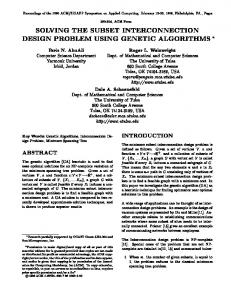
Figure 1: Setting the time windows for the drop-off location [an+i , bn+i ] given the pickup locations time window [ai , bi ], the direct transportation time ti,n+i from i to n + i, service time si at i and the upper limit on excess ride time E (Figure from [5]).
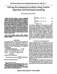
for different customers. Then the upper time limit for the drop off location becomes: bn+i = bi + si + ti,n+i + E. These time window calculations are shown in Figure 1. In the case of an outbound customer, the customer specifies the latest drop-off time, which is set as the upper limit on the drop-off time window, equal to bn+i . The other time window limits are then found using the same method backwards in time. Constraints (10) ensures that the vehicle capacity is not exceeded. In order to keep track of the number of seats needed for customers in each vehicle throughout the route, the term of load for each vehicle is introduced. The load of a vehicle at a point in time is the number of seats needed for the customers in the vehicle at that point in time. When a vehicle has serviced a pickup location i, the change in load is represented by li = ∆i and the change in load after servicing a drop-off location n + i is ln+i = −∆i . The actual load of vehicle k after servicing location i is Lki . The load of the vehicle after servicing the next location in the route, j, is then Lkj = Lki + lj . To make sure the capacity for a vehicle is not exceeded constraints (9) are introduced to the model. This ensures that the loads are correctly calculated for the edges used in the route. Finally, constraints (10) ensures that vehicle capacity is not exceeded and constraints (11) ensures that he actual loads of the vehicles are set to zero at the depots. The actual arrival time of a customer at the destination location depends on different factors in the objective function, such as the time window violation, excess ride time, ride time violation, route duration, route duration violation, and waiting time. If the customer arrives on time at his destination within the time windows, the cost contributed by the arrival of that customer is, if any, the excess ride time and the waiting time in an idle vehicle. On the other hand, if the customer is late, the time that passes from the upper bound of the time window to actual arrival is both the excess ride time and penalty for every minute the arrival time exceeds the upper time limit. If in addition the ride time of the customer exceeds the maximum ride time, a penalty is added to both the cost of excess ride time and time window violation. In this case we assume that the maximum ride time for the customer plus the pickup time is higher than the upper bound on the drop-off time window. This case is presented in Figure 2. Thus the cost of delivering a customer late increases in steps depending on the three constraints and of
6
upper time window
maximum ride time
Cost
direct transport time
α= w +w +w 3‘
6
7
α=w +w 3‘
α=0
6
α=w
3‘
Time
Figure 2: The influence of the arrival time on cost. The slope (α) of the cost increases in steps depending on the arrival time.
course on how late the customer is delivered. If a vehicle arrives too early at a location, it has to wait. Two cases may arise: 1) no customers are present in the vehicle; or 2) one or more customers are waiting in the vehicle. In the first case, the minutes the vehicle has to wait add a penalty to the cost for violating the time windows, the route duration increases, and a route duration violation may occur. The reason for penalizing a time window violation even though the vehicle is empty is to have the same implementation of the time window violation. If there are customers present in the vehicle, the waiting minutes will add to the cost in several ways: Penalty for time window violation, the waiting time multiplied by the number of customers present in the idling vehicle, excess ride time for the customers, route duration increases, and possibly ride time or route duration violations as well. The DARP can be proven to be N P-hard (see e.g. Baugh et al. [3]). The proof is based on the related N P-hard traveling salesman problem with time windows, into which the DARP can be transformed.
3 Related work This section contains a short description of previous work within the field of the DARP. The work mentioned here is selected based on its close relations to the problem definition and/or solution method found in this paper. 7
The work by Jaw et al. [6] in 1986 is generally considered pioneer research within DARP, and describes a sequential insertion heuristic algorithm. The objective function combines the minimization of operator costs and the minimization of customer inconvenience with respect to both customer ride time and deviation from desired pickup or drop-off times specified by each customer. The different parts of the objective function are balanced by multiplying them by user-specified constants. In the computational experiments the algorithm is tested on a number of simulated data sets with 250 customers, and 4 or 5 vehicles and real data sets with 2617 customers and 28 vehicles. The execution time for the simulated data set is about 20 seconds and about 12 minutes for the real data set. In Baugh et al. [3] the DARP is solved using simulated annealing. The work is based on the classical cluster-first, route-second approach. Customers are first organized into clusters and then the routes are developed for each individual cluster. The clustering is performed using simulated annealing while the routing is performed using a modified space-time nearest neighbour heuristic. The modified space-time nearest neighbour heuristic used to create routes for each cluster is a greedy algorithm. The results obtained are based on a set of real-life data set with 300 customers as well as on a generated data set with 25 customers. No CPU times are given in the paper. It is claimed by the authors that the algorithm gives near globally optimal solutions. Cordeau and Laporte [5] describe a tabu search heuristic. Their algorithm initiates with a randomly generated initial solution. In order to avoid cycling, solutions possessing attributes of recently visited solutions, are put on the tabu list and are therefore forbidden for a number of iterations. Infeasible solutions may be explored during the search, as constraints are relaxed and violations are added to the objective function. After each iteration the parameters are dynamically adjusted. The objective function consists of the total transportation cost of the vehicles and the violation terms. Three variants of the heuristic were tested using both randomly generated data sets with 24 to 144 customers and six real-life data sets containing either 200 or 295 customers. The execution times for the randomly generated data sets are about 2 minutes for the smallest data sets and up to 93 minutes for the largest data sets. The execution times for the real-life data sets are given to be between 13 and 268 minutes. Jih et al. [7] solve the single vehicle pickup and delivery problem with time windows using a genetic algorithm. In the algorithm the chromosome representation of a route is defined by letting the chromosome represent the locations in a traveling sequence of the route. The algorithm permits exploration of infeasible solutions during the search. The objective function is the sum of the total travel cost of the vehicle and the penalty for violating constraints. Four different types of crossover are considered. The algorithm is tested on randomly generated data sets with up to 100 customers. Execution time is about 38 minutes for the largest data sets. The results of the algorithm are compared with the optimal values which are available for the smaller data sets (up to 40 customers). The best results for the genetic algorithm are obtained by using the uniform order-based crossover. It is able to reach the optimum on the average in 83% of the runs for the data sets with up to 40 customers. 8
Paper
Algorithm
Objectives
[6]
sequential insertion heuristic
min operator costs, min customer ride times, min deviation from time windows
[3]
cluster-first routesecond, simulated annealing
min total distance, min number of vehicles, min inconvenience
[5]
Tabu Search
min transportation cost, min penalty violations
[7]
Genetic Algorithm
min transportation cost, min penalty violation
size 250
Test results type time random 20 sec.
2617 25
real-life random
12 min. n.a.
300 144
real-life random
n.a. 93 min.
295 100
real-life random
768 min. 38 min.
Table 1: Overview of previous related work for the DAR problem. Note that [7] solves the related Pickup-and-Delivery problem.
4 The Genetic Algorithm Genetic Algorithms (GA) have shown good performance on a number of related routing problems (see eg. [11, 9]). It was therefore an obvious choice for the clustering level in our two-phase approach. GA is based on maintaining a set of solutions, called a population. Therefore an initial population generator is needed before the GA can start. In this case, the GA begins by creating an initial population, in which all the customers are clustered randomly. For an in-depth introduction into GA see [10]. One way of implementing a genetic algorithm for the DARP in one step is to adopt the chromosome representation used in Pereira et al. [9]. In the chromosome representation both the allocation of customers to vehicles and the order of the customers on the routes are encoded. The representation is used when solving the vehicle routing problem but the extension to the DARP is problematic. The main obstacles are the precedence constraints (5) and (6). In order to solve this problem some elaborate fix-up would be needed each time a new individual is created. Instead the classical split in clustering and routing is used. In the clustering part as many groups of customers as there are available transportation vehicles are created. Each customer can only belong to one group and only one group can be assigned to each vehicle. The clustering of customers is solved using the genetic algorithm. When all the 9
customers have been grouped, a route for each vehicle is constructed. The routing involves deciding the order of the stops of the vehicle as well as the time table for the vehicle. The routing is solved using an extended version of the modified space-time nearest neighbor heuristic developed by Baugh et al. [3]. Figure 3 presents an overview of the solution process. Initial population constructed
Routes developed and cost calculated
GA
NO
END
YES
STOP
Figure 3: An overview of the solution process.
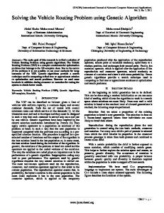
The construction of the GA involves decisions regarding which chromosome representation fits the solution to the problem, which population size is adequate, how the initial population should be generated, what stopping criteria to use, how the fitness calculations should be made, what kind of selection mechanism is superior, and which modifying operators to use. In order for an individual in the population to represent a solution to the problem of allocating customers to vehicles it is decided to use a two level binary chromosome representation. The representation is set up as a matrix. There are as many rows as there are available vehicles and there are as many columns as there are customers and depots. A 1-entry at any position [g1, g2] indicates that the customer/depot represented by column g1 is allocated to the vehicle represented by row g2. It is very easy to verify that each customer is allocated to exactly one vehicle. Figure 4 shows an example of what the chromosome representation looks like when there are four vehicles available, one depot and 16 customers. The routes can be constructed in many ways e.g. as shown in Figure 5. The size of the population greatly influences the performance of the GA. If the population size is too small it results in a high possibility of an under-covered solution space, while too large a population is a burden on the computational time and may lead to an 10
de po cu t s to cu me r1 st o cu m e st r2 o cu m e r st 3 o cu m e r st 4 cu o m s t er c u om 5 s to e r 6 c u me s to r 7 c u me r8 st cu o me st o r9 cu m e r st om 1 0 er cu st 11 o cu me r1 st cu o m e 2 st o r 1 cu m e 3 st o r 1 4 m er cu s to 15 m er 16 Route 1
1
0
1
0
1
0
0
0
1
1
1
0
0
1
0
1
0
Route 2
1
1
0
0
0
1
1
0
0
0
0
0
1
0
0
0
0
Route 3
1
0
0
1
0
0
0
0
0
0
0
0
0
0
1
0
0
Route 4
1
0
0
0
0
0
0
1
0
0
0
1
0
1
0
0
1
Figure 4: An example of the binary chromosome representation used in the solution method. There are as many columns as customers and depots and as many rows as routes. The number of routes equals the number of available vehicles. Each customer must be assigned to exactly one route and each route has to include the depot. depot - 9.1 - 15.1 - 15.2 - 2.1 - 9.2 - 8.1 - 10.1 - 8.2 - 2.2 - 10.2 - 13.1 - 13.2 - 4.1 - 4.2 - depot
Figure 5: A possible route based on the clustering of Figure 4, where the i.1 is the pickup location of customer i and i.2 is the drop off location of customer i, for all i in route 1. unacceptable slow rate of convergence. It is decided to use the conventional method of a constant population size and perform some preliminary tests to decide how big the population size should be for the problems that are to be solved. The algorithm terminates after a fixed number of iterations. One parent is chosen by means of a stochastic procedure, while the second parent is chosen randomly. The stochastic procedure, also called the roulette wheel method, gives each individual in the current population a probability of being chosen as parent proportional to the fitness value of the individual. In each iteration one offspring is created, which replaces one random member belonging to the Z portion of the current population, consisting of the individuals with the worst fitness values, i.e. which represent solutions with high cost. Z is set to be proportional to the population size and different values for Z will be tested. This method for updating the population is called incremental replacement and the best member of a current population is guaranteed to survive to the next population. The crossover used in the algorithm is a version of the crossover described by Pereira et al. [9]. In this crossover, one row, i.e. one cluster, is chosen at random from both parents and a random binary template is created. The template is used as a recipe for one row in the offspring, where a 1-entry in the template indicates that the gene is to be taken from parent 2. The offspring consists of the new row while the other rows are duplicates from parent 1. When constructing a new solution with the crossover operator as described above, the 11
resulting solution is not necessarily a legal solution. Therefore it is examined whether a customer exists which is assigned to more than one vehicle or no vehicle at all. If such a customer is found, a cluster is chosen randomly and the customer is either added or deleted from that cluster depending on whether the customer is allocated too often or not at all. If the randomly chosen cluster is the cluster created in the crossover a new cluster is randomly chosen. This procedure is repeated until all the customers are allocated to exactly one vehicle. It is not necessary to verify that the depot is present in every cluster since the parents represent a legal clustering solution. In each iteration one crossover is performed resulting in one offspring. If parent 2 turns out to be the better parent, the parent numbering is switched, so that parent 1 always represents a better individual than parent 2. Initially the template was generated completely randomly but tests indicate that increasing the probability of selecting genes from parent 1 yields better results. Preliminary results show that a big increase of the probability is not sensible, especially in the beginning of the iterations, therefore the probability of choosing genes from parent 1 (the better parent) is set to 60%. The mutation operator moves one random customer from its current cluster to another random cluster. It is not possible to generate illegal solutions using this mutation so no verification or correction procedure is needed after mutation. The offspring that has been created in the crossover can be subjected to mutation with a certain probability, called the mutation probability, Pµ . As duplicates distort the selective process and waste computational resources, they are to be avoided if possible. In our algorithm the probability of duplicate chromosomes is reduced by mutating the offsprings that have the same fitness values as their parent 1 and therefore represent the same solution. si
t i,n+i
Service time
Direct transportation time an+i
Latest pickup time
Latest possible departure from pickup location
Lower bound on drop−off TW
b n+i
Time
Upper bound on drop−off TW
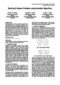
Figure 6: Illustration of the latest pickup time calculations for an outbound customer. The latest pickup time is calculated backwards in time. The direct transportation time from pickup to drop-off location and the service time at the pickup location are subtracted from the upper bound on the drop-off time window.
Now clusters of customers have been generated using the GA in the first phase of the solution method. In the second phase routes are constructed for the clusters and costs evaluated. The modified space-time nearest neighbor heuristic (Baugh routing-heuristic) 12
Routes developed and cost calculated
Initial population constructed
Population updated − if needed
STOP
YES
END
NO Mutation − new solution
Parents selected NO
YES
MUTATE
Crossover − new solution
Figure 7: An overview of the initial heuristic
described by Baugh et al. [3] is used, in an extended version, for developing routes and calculating cost for each route. It is used as it displays excellent results. In the Baugh routing-heuristic the cost of a route is set to be the weighted sum of travel time and time window violations. The hard constraints that are included into the heuristic are the routing, precedence and capacity constraints. The depot constraints, maximum route duration, and maximum ride time constraints are not included. Neither are excess ride times, waiting times with passengers in idle vehicles nor route duration constraints. The remaining constraints and cost factors are included directly in the heuristic in this paper. Service times at each location are also included in the heuristic. The method of choosing the first customer in a route is also altered from the original procedure. In the Baugh routing-heuristic the first customer is chosen to be the customer with the earliest pickup time, which does not give good results for the data used here, since some of the pickup locations have no associated time window which is the case for outbound customers. This means that the time window is set to the whole planning horizon ([0, T ]) and the lower time window is zero. Therefore outbound customers are often chosen as first customers, as the drop-off time has no influence. In order to account for this, the first serviced customer is instead chosen to be the customer with the earliest upper time limit in the pickup time window. For customers with no pickup time windows, latest pickup times, based on the drop off time windows, are assigned. The latest pickup times for these customers are the upper time limit for the drop-off location subtracted by direct transportation time and service time at the pickup location. An illustration of the latest pickup time calculations for an outbound customer is shown in Figure 6. Figure 7 gives an overview of the structure of the heuristic.
13
5 Experimental results There are as yet no well-known and established benchmarks available in the literature of the version of DARP used in this project. The behavior of the solution method proposed here can therefore not be tested using data instances that have been widely tested and the results cannot be compared to the optimum or the best results obtained in previous publications. The test instances used for testing the solution method proposed here are obtained from Cordeau and Laporte [5]. They created the test instances to analyze the behavior of the simulated annealing when solving the DARP. Cordeau and Laporte generated a set of 20 random test instances (data sets) according to realistic assumptions. The information regarding time window widths, vehicle capacity, route duration, and maximum ride time were provided by the Montreal Transit Commission (MTC). In the test instances there are between 24 and 144 customers. The first half of the customers is assumed to consist of outbound customers while the remainder of the customers are assumed to be inbound. For each instance, the origin and destination locations are generated using a procedure that creates clusters of vertices around a certain number of seed points. All instances contain a single depot and the location of the depot is set at the average location of the seed points. For a more detailed description of this procedure, we refer to Cordeau et al. [4]. For each instance the service time (si ) in each location i (i ∈ N) is equal to 10, and the load change, li , in each location i is either 1 or −1. 1 for the pickup locations and −1 for the drop-off locations, i.e. no customer has companions traveling with them, and all the customers demand only one seat. The depot location, on the other hand, has a service time and load change equal to zero, since no customers are entering or leaving the vehicle at the depot. Further, the maximum route duration, r k , is equal to 480 in all instances, vehicle capacity, C k , is equal to 6, and the maximum ride time, ui , is equal to 90. A time window [ai , bi ] is generated for each location. As mentioned in Section 2, the origin point of an inbound customer and the destination point of an outbound customer are subject to time windows, while the other points have no customer specific time windows associated with them. The time windows for these points are therefore set to [0, T ], where T is the planing horizon, which in these experiments is equal to 1440 = 24x60, i.e. the number of minutes in one day. Two groups of customer specific time windows are constructed in the data sets. The first one has narrow time windows while the second one has wide time windows. The narrow time windows are constructed by choosing an uniform random number, ai , in the interval [60, 480] and then choosing another uniform random number, bi , in the interval [ai + 15, ai + 45]. For the wide time windows group ai is chosen in the same manner but bi is chosen in the interval [ai + 30, ai + 90], resulting in time windows [ai , bi ] (i ∈ N). The test instances R1a to R10a have narrow time windows while test instances R1b to R10b have wide time windows. Test instances R1a to R6a and R1b to R6b are generated so that the number of available vehicles in comparison to the number of customers is higher than in test instances R7a to 14
Instances R1a R2a R3a R4b R5a R6a R07a R9a R10a
R1b R2b
R5b R6b R07b R9b R10b
Customers Vehicles 24 3 48 5 72 7 96 9 120 11 144 13 36 4 108 8 144 10
Table 2: Size of data instances used in tests Population size M Iteration number G Mutation probability Pµ Proportion replaced Z
50 15000 0.01 0.10
Table 3: Fixed parameters
R10a and R7b to R10b, e.g. R6a has 13 available vehicles while R10a has 10 available vehicles, both instances having 144 customers. All the test instances constructed by Cordeau and Laporte are available from the Internet at http://www.hec.ca/chairedistributique/data/darp/. We are only considering the instances where the necessary information for a comparison is present. Problems in Table 2 have a given solution except R4b and R7a, which will be used in parameter tuning. Table 2 gives the number of customers and available vehicles in the test instances that are used in this paper. The distance between any two locations i and j is set to be the Euclidean distance between the coordinates of locations i and j, i, j ∈ A. The speed of the vehicles is set to 1, so the transportation time ti,j is equal to the Euclidean distance between i and j. So the first term in the objective function 1 now equals the total weighted transportation distance. Through an extensive set of tests, good values for the population size, number of iterations, multation probability, and proportion of population that is replaced have been found. The parameters are fixed at the values reported in Table 3. A more in-depth description of the tests can be found in [2]. Of course, the more iterations that are run, the better solutions are obtained. The chosen number of iterations defines a good compromise between time and quality. Running e.g. 30000 iterations resulted in execution times of around 150 minutes, which is too much for a practical setting. 15
The customers naturally emphasize the level of service provided by the transportation operator. They want the bus to arrive on time and the ride time to be minimal. On the other hand they do not want the service to be very expensive and therefore they set their demands on service to reasonably high levels in their opinion. After performing some preliminary testing the resulting weights are: w1 = 8,
w2 = 3,
w3 = 1,
w4 = 1,
w5 = n,
w6 = n,
w7 = n
The weights on violating the relaxed constraints presented in the objective function (1) are set to n, i.e. the total number of customers in each data instance, because the values for the cost factors for distance, route duration and ride time increase proportionally with the number of customers. The value of the cost terms for the relaxed constraints is not as dependent on the number of customers as the above mentioned factors. The weight on customers transportation time is set to 8, as the customers are concerned with the transportation time. The weight on excess ride time (w2 ) is set to 3, as the customers consider it important that transportation time is short. The weights on waiting time with customers (w3 ) are set to 1, because the customers generally do not mind waiting in the vehicle as long as the excess ride time is reasonable. The weight on work time (w4 ) is also set to 1, because the size of the route duration is large compared to the other segments in the fitness function and the customers are not very concerned with the route duration, as they only share part of the route. In all tests, each instance is run 5 times and we present the average results from the data obtained in these runs along with the best total cost found for each instance. The results obtained using the genetic algorithm is compared to the results obtained by Cordeau and Laporte [5]. The average results from the best improved heuristic are presented in Table 4 along with the results for the best solution obtained for each data set (i.e. the solution with the lowest cost). The vehicle waiting time is not critical in this model, since it is not a part of the objective to minimize the vehicle waiting time but rather customer waiting time. Cordeau and Laporte [5], on the other hand, report this waiting time which is the reason it is included in Table 4. The best solution results are somewhat different from the average results of Cordeau and Laporte [5]. Route duration is 14% higher, waiting time 40% lower, and ride time 9% lower in the solution presented here. Cordeau and Laporte [5] performed 104 to 105 iterations in order to get their best results which are presented in Table 5. In the testing in this paper, 15000 iterations are performed. The total CPU time is however comparable. Cordeau and Laporte [5] use an Intel Pentium 4, 2 GHz processor in their CPU measurements and in this paper, results are obtained on an Intel Celeron 2 GHz processor. 99% of the CPU time spent on the test cases in this paper is used by the routing heuristic. The objective function used by Cordeau and Laporte [5] is: v(S) = v1 (S) + αv2 (S) + βv3 (S) + γv4 (S) + τ v5 (S)
(13)
where v(S) is the objective value for solution S. The function v1 (S) denotes the total routing cost of the vehicles, v2 (S) denotes total load violation, v3 (S) denotes total route 16
Route duration Avg. Best R1a R2a R3a R5a R9a R10a R1b R2b R5b R6b R7b R9b R10b Total
1041 1969 2779 4250 3597 5006 907 1719 4296 5309 1299 3679 4733 40584
1039 1994 2781 4274 3526 5025 928 1710 4336 5227 1316 3676 4678 40508
Vehicle waiting time Avg. Best total avg total avg 252 5.25 260 5.42 470 4.90 514 5.36 292 2.03 301 2.09 500 2.08 527 2.20 94 0.44 32 0.15 315 1.09 246 0.86 143 2.98 164 3.42 198 2.06 162 1.69 552 2.30 568 2.37 630 2.19 513 1.78 102 1.41 128 1.78 147 0.68 177 0.82 113 0.39 85 0.29 3808 27.81 3678 28.21
Ride time Avg. total avg 477 19.86 1367 28.47 3081 42.79 5099 42.49 6251 57.88 8413 58.42 630 26.24 1214 25.30 4615 38.46 6134 42.59 990 27.50 5362 49.65 7969 55.34 51600 514.99
Best total avg 310 12.90 1330 27.72 2894 40.20 4837 40.30 6719 62.21 8341 57.92 549 22.89 1300 27.07 4720 39.33 6397 44.42 784 21.76 5358 49.61 8119 56.38 51657 502.72
Table 4: The results obtained by the genetic algorithm.
Route Vehicle wait. time Ride time CPU duration total avg total avg [min] R1a 881 211 4.4 1095 45.62 1.90 R2a 1985 724 7.54 1977 41.18 8.06 R3a 2579 607 4.22 3587 49.82 17.18 R5a 3870 833 3.47 6154 51.3 46.24 R9a 3155 323 1.5 5622 52.05 50.51 R10a 4480 721 2.5 7164 49.75 87.53 R1b 965 321 6.68 1042 43.4 1.93 R2b 1565 309 3.22 2393 49.86 8.29 R5b 3596 606 2.52 6105 50.87 54.33 R6b 4072 449 1.56 7347 51.02 73.70 R7b 1097 129 1.79 1762 48.94 4.23 R9b 3249 487 2.26 5581 51.68 51.28 R10b 4041 362 1.26 7072 49.11 92.41 Total 35537 6082 42.92 56900 634.6 497.59 Table 5: Results obtained by Cordeau and Laporte [5].
17
CPU time [min] 5.57 11.43 21.58 58.23 40.78 65.98 5.46 11.72 58.93 81.23 8.29 44.66 66.41 488.61
duration violation, v4 (S) denotes total time window violation, and v5 (S) denotes total ride time violation. α, β, γ, and τ are a self-adjusting weights. The values of these weights change in each iteration and no approximate values are given in the paper. Neither is the method used to calculate the total routing cost specified in the paper, which makes it impossible to evaluate the comparison of the total costs obtained by the two solution methods. As mentioned previously, the route duration is higher in our algorithm than in Cordeau and Laporte [5]. The other two results, which are related to customer service, ride time, and vehicle waiting time are on the other hand better than in the results obtained by Cordeau and Laporte [5]. One reason for these results is that, in this paper, the weights are set to represent the choice of the customers so there is an emphasis on customer service factors.
6 Conclusion and further research This paper has presented an implementation of a new heuristic approach for solving the DARP, using the classical cluster-first route-second framework. A genetic algorithm was used for the clustering phase, and a modified space-time nearest neighbor heuristic was used in the routing part. The resulting method was compared to the results given by Cordeau and Laporte [5]. The comparison focused on route duration, as well as ride and vehicle waiting times. The comparison showed that Cordeau and Laporte [5] obtain better results for route duration whereas the genetic algorithm approach presented here obtains better results with regards to ride time and vehicle waiting time. The results are overall comparable to those obtained by Cordeau and Laporte [5], where differences are explained by the setting of cost vs. service level parameters. The improvements to the genetic algorithm introduced in Section 4 regarding the reduction of randomness, have shown to give very good results, and several ideas concerning further improvements are still untested. One possibility is to use ranking when selecting parents in the genetic algorithm and to experiment with different crossover and mutation operators. Also, to improve computational time, a different routing algorithm could be implemented. The modified space-time nearest neighbour heuristic used 99% of the CPU time which of course set a rather low limit on the number of iterations the genetic algorithm could perform. The overall conclusion of this paper is that the new solution method for solving the DARP, which is presented here, shows some promising results. It is possible to adjust the weights of seven factors concerning cost of operation vs. level of service, which enables evaluation of consequences in different dial-a-ride scenarios. The new solution method has achieved solutions comparable to the current state-of-the-art methods.
18
References [1] R. Borndorfer, M. Grotschel, F. Klostermeiner and C. Kuttner. Telebus Berlin: Vehicle Scheduling in a Dial-a-Ride System. Konrad-Zuse-Zentrum fur Informationstechnik Berlin, 1997. [2] Kristin Berg Bergvinsdottir. The Genetic Algorithm for solving the Dial-a-Ride Problem. Masters Thesis. Informatics and Mathematical Modelling, Technical University of Denmark, 2004. [3] J.W. Baugh jr., D.K.R. Kakivaya and J.R. Stone. Intractability of the dial-a-ride problem and a multiobjective solution using simulated annealing. Engineering Optimization, 30(2):91 - 124, 1998. [4] J.F. Cordeau, M. Gendrau and G. Laporte. A tabu search heuristic for periodic and multi-depot vehicle routing problems. Networks 30, 105 - 119, 1997 [5] J.F. Cordeau and G. Laporte. A tabu search heuristic for the static multi-vehicle dial-a-ride problem. Transportation Research, Part B, 37:579 - 594, 2003. [6] J.J. Jaw, A.R. Odoni, H.N. Psaraftis and N.H.M. Wilson. A heuristic algorithm for the multi-vehicle advance request dial-a-ride problem with time windows. Transportation Research, Part B (Methodological), 20B(3):243 - 257, 1986. [7] W.R. Jih, C.Y. Kao and F.Y.J. Hsu. Using Family Competition Genetic Algorithm in Pickup and Delivery Problem with Time Window Constraints. In Proceedings of the 2002 IEEE International Symposium on Intelligent Control, Vancouver, Canada, 496 - 501, 2002. [8] R.M. Jorgensen. Dial-a-Ride. Doctor’s thesis, Technical University of Denmark, 2002. [9] F.B. Pereira, J. Tavares, P. Machado and E. Costa. GVR: a New Genetic Representation for the Vehicle Routing Problem. Artificial Intelligence and Cognitive Science. 13th Irish Conference, AICS 2002. Proceedings (Lecture Notes in Artificial Intelligence Vol. 2464), 95 - 102, 2002. [10] C.R. Reeves. Modern Heuristic Techniques for Combinatorial Problems. McGrawHill International Limited UK, 151 - 188, 1995. [11] Jörg Homberger and Hermann Gehring. Two evolutionary metaheuristics for the vehicle routing problem with time windows. INFOR, 37(3): 297 - 318, 1999.
19