Jul 30, 2012 - arXiv:1207.6811v1 [nucl-th] 30 Jul 2012. Solving the heat-flow problem with transient relativistic fluid dynamics. G. S. Denicola, H. Niemib, ...
Solving the heat-flow problem with transient relativistic fluid dynamics G. S. Denicola , H. Niemib , I. Bourasa, E. Moln´ arc,d, Z. Xue , D. H. Rischkea,c , and C. Greinera a
arXiv:1207.6811v1 [nucl-th] 30 Jul 2012
d
Institut f¨ ur Theoretische Physik, Johann Wolfgang Goethe-Universit¨ at, Max-von-Laue-Str. 1, D-60438 Frankfurt am Main, Germany b Department of Physics, P.O. Box 35 (YFL) FI-40014 University of Jyv¨ askyl¨ a, Finland c Frankfurt Institute for Advanced Studies, Ruth-Moufang-Str. 1, D-60438 Frankfurt am Main, Germany MTA-KFKI, Research Institute of Particle and Nuclear Physics, H-1525 Budapest, P.O.Box 49, Hungary and e Department of Physics, Tsinghua University, Beijing 100084, China Israel-Stewart theory is a causal, stable formulation of relativistic dissipative fluid dynamics. This theory has been shown to give a decent description of the dynamical behavior of a relativistic fluid in cases where shear stress becomes important. In principle, it should also be applicable to situations where heat flow becomes important. However, it has been shown that there are cases where IsraelStewart theory cannot reproduce phenomena associated with heat flow. In this paper, we derive a relativistic dissipative fluid-dynamical theory from kinetic theory which provides a good description of all dissipative phenomena, including heat flow. We explicitly demonstrate this by comparing this theory with numerical solutions of the relativistic Boltzmann equation. PACS numbers: 12.38.Mh, 25.75.-q, 11.25.Tq
I.
INTRODUCTION
The derivation of a consistent theory of relativistic fluid dynamics has been a challenge for some time. The difficulty resides in the parabolic nature of Navier-Stokes theory, which allows signals to propagate with infinite speed. While in non-relativistic theories this unphysical feature can be dismissed, in relativistic systems it leads to unstable equations of motion and is simply unacceptable [1]. A necessary (but not sufficient) condition is that the equations of motion are hyperbolic. For relativistic dilute gases, the Boltzmann equation provides a reasonable description of the underlying microscopic theory and can serve as a starting point to investigate the microscopic foundations of fluid dynamics. For the sake of simplicity, in this paper we consider a single-component system of massless and classical particles interacting only via elastic two-body collisions with a constant cross section σ. The relativistic Boltzmann equation for this type of system reads Z 1 µ k ∂µ fk = (1) dK ′ dP dP ′ Wkk′→pp′ (fp fp′ − fk fk′ ) , 2 where �fk is the� single-particle distribution function, Wkk′→pp′ is the Lorentz-invariant transition rate, and dK ≡ gd3 k/ (2π)3 k 0 is the Lorentz-invariant momentum-space volume, with g being the number of internal degrees of freedom. The right-hand side of the Boltzmann equation describes the change of the single-particle distribution function due to elastic collisions of two particles with incoming momenta k and k ′ , and outgoing momenta p and p′ . The conservation laws follow from the first two moments of the Boltzmann equation as a consequence of the conservation of particle number and energy-momentum in individual collisions, ∂µ N µ = 0, ∂µ T µν = 0. The particle four-current, N µ , and the energy-momentum tensor, T µν , can be cast in the usual form, N µ = nuµ + nµ , T µν = εuµ uν − P0 ∆µν + π µν ,
(2)
where n is the particle number density, nµ is the particle diffusion four-current, ε is the energy density, uµ is the fluid four-velocity defined in the Landau frame [2], i.e., uν T µν = εuµ , P0 is the thermodynamic pressure, and π µν is the shear-stress tensor. Since we consider a massless gas, the bulk viscous pressure is always zero. The additional equations needed in order to solve the conservation laws, i.e., the equations of motion for nµ and π µν , must be derived by properly matching fluid dynamics to the relativistic Boltzmann equation. In the framework of relativistic kinetic theory, Israel and Stewart were among the first to derive a relativistic theory of fluid dynamics that is causal and stable [3]. In the Israel-Stewart (IS) formulation, the single-particle distribution function is expanded around its local equilibrium value in terms of a series of Lorentz tensors formed of particle four-momentum k µ , i.e., 1, k µ , k µ k ν , . . .. In order to derive fluid dynamics, this series is truncated at second order in momentum, i.e., one only keeps the tensors 1, k µ , and k µ k ν , the so-called 14-moment approximation. The 14 coefficients of this truncated expansion are uniquely matched to the 14 components of N µ and T µν . Finally, the equations of motion for nµ and π µν are obtained by substituting the truncated moment expansion into the second moment of the Boltzmann equation.
2 In the past five years, IS theory has been widely applied to ultrarelativistic heavy-ion collisions in order to describe the time evolution of the quark-gluon plasma (QGP) and the freeze-out of the hadron resonance gas appearing in the late stages of the collision. However, in heavy-ion collisions extreme conditions occur which question the validity of fluid dynamics. The QGP created at the Relativistic Heavy Ion Collider (RHIC) and, recently, at the Large Hadron Collider (LHC) is not only the fluid with the smallest space-time extension (∼ 10 fm) ever created in nature but also the one where the space-time gradients of the fluid fields, for instance energy density ε, are the largest (∼ |∂µ ε|/ε ∼ 1/fm) ever encountered. On the other hand, Israel and Stewart’s derivation lacks a small parameter, such as the Knudsen number, with which one can do power counting and systematically improve the approximation to describe higher-order gradients. Thus, the applicability of IS theory to the extreme conditions reached in heavy-ion collisions is, at the very least, not clear. One way to investigate the applicability of IS theory is to compare the solutions of this theory with numerical solutions of the Boltzmann equation [4–8]. So far, it was confirmed that, at least for some special problems, the IS equations [3] are not in good agreement with the numerical solution of the Boltzmann equation. In these cases, it was shown by some of the present authors [6] that the IS formalism seems to be unable to describe heat flow, even when the Knudsen number is very small. In this paper, we would like to explain the reason for this discrepancy and propose a solution which works at least if the Knudsen is not too large. Recently, a systematic derivation of fluid dynamics from the Boltzmann equation was introduced in Ref. [9]. The main difference between IS theory and the theory derived in Ref. [9] is that the latter does not truncate the moment expansion of the single-particle distribution function. Instead, dynamical equations for all its moments are considered and solved by separating the slowest microscopic time scale from the faster ones. Then, the resulting fluid-dynamical equations are truncated according to a systematic power-counting scheme using the inverse Reynolds number R−1 ∼ |nµ | /n ∼ |π µν | /P0 and the Knudsen number Kn = λmfp /L, with λmfp being the mean free-path and L a characteristic macroscopic distance scale, e.g. L−1 ∼ ∂µ uµ . The values of the transport coefficients of fluid dynamics are obtained by resumming the contributions from all moments of the single-particle distribution function, similar to what happens in the Chapman-Enskog expansion [10]. In this paper, we review the basic aspects of this resummed transient relativistic fluid-dynamical theory (RTRFD). We explicitly derive the equations of motion of RTRFD including terms up to second order in the Knudsen number. We then demonstrate that this method is also able to handle problems with strong initial gradients in pressure or particle number density. This resolves the previously observed differences between the solution of IS theory and of the Boltzmann equation [6] mentioned above. We conclude that these differences were caused by the uncontrolled truncation procedure of the expansion of the single-particle distribution function in terms of Lorentz tensors in fourmomentum as employed in IS theory. This paper is organized as follows. In Sec. II, we review the basic aspects of RTRFD. One important point is that the fluid-dynamical equations of motion, as derived in Ref. [9], become parabolic once second-order terms in Knudsen number are included. In Sec. III, we explain how to obtain hyperbolic equations of motion in the RTRFD formalism up to second order in the Knudsen number. In Sec. IV, we compare solutions obtained within RTRFD for various levels of approximation and within IS theory with numerical solutions of the Boltzmann equation computed using BAMPS [11]. In Sec. V we discuss our results and draw conclusions. The Appendix contains intermediate steps of our calculations. We use natural units ~ = c = kB = 1. The metric tensor is gµν = diag (+, −, −, −). II.
REVIEW OF RESUMMED TRANSIENT RELATIVISTIC FLUID DYNAMICS
In RTRFD [9], fk is expanded in terms of an orthonormal and complete basis in momentum space. The expansion basis contains two basic ingredients: The first are the irreducible tensors, 1, k hµi , k hµ1 k µ2 i , . . . , k hµ1 · · · k µm i , which form a complete and orthogonal set, analogously to the spherical harmonics [9, 12, 13]. Here, we use the notation ···µℓ ν1 ···νℓ ···µm µ Ahµ1 ···µℓ i ≡ ∆µν11···ν , with ∆µν11···ν m . The latter quantities are projectors onto the subspaces orthogonal to u . ℓ A µ µ µ Their definition is explicitly given in Refs. [9, 12]. Except for m = 1, where ∆ν = gν − u uν , they are traceless. E.g., µ ν µ ν µν for m = 2, ∆µν αβ = (∆α ∆β + ∆β ∆α )/2 − ∆ ∆αβ /3. Note that the expansion of fk in IS theory is not in terms of the µm i hµ1 ···k , but in terms of the tensors k µ1 · · · k µm which are complete but neither irreducible irreducible tensors k nor orthogonal. P (ℓ) (ℓ) The second ingredient are orthogonal polynomials in Ek = uµ kµ , Pnk = nr=0 anr Ekr . For details in constructing the polynomials, see Ref. [9]. Then, fk is expanded as fk = f0k + f0k
Nℓ ∞ X X
(ℓ)
Hnk ρµn1 ···µℓ khµ1 · · · k µℓ i ,
(3)
ℓ=0 n=0
where f0k = exp (α0 − β0 Ek ) is the local equilibrium distribution function, with α0 = µ/T being the ratio of chemical
3 potential to temperature and β0 = 1/T the inverse temperature. We further introduced the energy-dependent � PNℓ (ℓ) (ℓ) (ℓ) (ℓ) , and the irreducible moments of coefficients Hnk ≡ W (ℓ) /ℓ! m=n amn Pmk , with a normalization constant W δfk = fk − f0k , Z (4) ρµr 1 ···µℓ ≡ dK Ekr k hµ1 · · · k µℓ i δfk . µ µν µ µν Some of the irreducible moments are related to the fields in Eq.
(2): � n = ρ0 and π R= ρ0 . The values of α0 and 2 β0 are defined by the matching conditions, n ≡ hEk i0 , ε ≡ Ek 0 , where h· · · i0 ≡ dK (· · · ) f0k . The matching conditions and the definition of uµ according with the Landau picture imply that the following moments should vanish: ρ1 = ρ2 = ρµ1 = 0. The equations of motion for ρµr and ρµν r together with their respective transport coefficients were derived in Ref. [9]. Since we are investigating the massless limit, the scalar moments ρr will not play a dominant role (they contribute mainly to the bulk viscous pressure) and we set them to zero. We also neglect all irreducible moments with tensor rank higher than 2, since they are traditionally not considered in fluid dynamics. The role of such moments will be investigated in a future work. Then, the equations for the first- and second-rank tensors ρµr and ρµν r read
ρ˙ hµi r
+
Nℓ X
µ (1) µ ν µ A(1) rn ρn = αr I + ρr ω ν −
n=0,6=1
ρ˙ rhµνi +
Nℓ X
µν (2) µν A(2) − rn ρn = 2αr σ
n=0
2r + 3 ν µ β0 Ir+2,1 µ r+3 µ µν ∆ ∂λ π λν , ρr θ − ∆µλ ∇ν ρλν ˙ν − ρr σν + r−1 + rρr−1 u 3 5 ε0 + P0 ν
2 2 r + 4 µν 2 νi νi νi hµ (2r + 5) ρλhµ σλ + 2ρλhµ ω λ + ∇hµ ρr+1 − (r + 5) ρr+1 u˙ νi − ρr θ, r r 7 5 5 3 (5)
hµ ···µ i
···µℓ µ where ρ˙ r 1 ℓ ≡ ∆µν11···ν u ∂µ ρrν1 ···νℓ , I µ = ∇µ α0 , σ µν = ∂ hµ u νi , and ∇µ = ∂ hµi [9]. We also defined the thermodyℓ namic integrals Z �q 1 dKEkn−2q −∆αβ kα kβ f0k . (6) Inq (α0 , β0 ) = (2q + 1)!!
The coefficients
Z 1 dKdK ′ dP dP ′ Wkk′→pp′ f0k f0k′ f˜0p f˜0p′ Ekr−1 k hν1 · · · k νℓ i 4ℓ + 2 � � (ℓ) ′ (ℓ) ′ (ℓ) ′ ′ (ℓ) · · · p p · · · p − H · · · k − H p × Hkn khν1 · · · k νℓ i + Hk′ n khν ′ νℓ i pn hν1 νℓ i νℓ i p n hν1 1
(ℓ) Arn =
(7)
(ℓ)
contain all the information of the microscopic theory, while αr are complicated functions of β0 and α0 [9]. We now identify the microscopic time scales that dominate the long-time dynamics of the Boltzmann equation. This can be achieved by finding the normal modes of Eqs. (5), i.e., by diagonalizing the matrices A(ℓ) . Then, one obtains the following (in the linear regime, decoupled) set of equations of motion, µ (1) µ µ X˙ rhµi + χ(1) r Xr = βr I + Xr ,
(ℓ)
µν (2) µν X˙ rhµνi + χ(2) + Xrµν , (8) r X r = βr σ � P (ℓ) Nℓ −1 and Xrµ1 ···µℓ ≡ ρµ1 ···µℓ are the eigenmodes of the linearized j=0 Ω rm m
are the eigenvalues of A(ℓ) �(ℓ) (ℓ) (ℓ) (ℓ) (ℓ) Boltzmann equation, with Ω−1 A Ω = diag(χ0 , . . . , χr , . . .). The terms Xrµ and Xrµν represent nonlinear (ℓ) terms and terms containing derivatives of the eigenmodes. The coefficients βr are complicated functions of α0 and β0 [9]. Without loss of generality, we order the eigenmodes of the linearized Boltzmann equation, Xrµ1 ···µℓ , according (ℓ) (ℓ) (ℓ) to increasing χr , i.e., in such a way that χr < χr+1 , ∀ ℓ. µν µ It is clear that when the terms Xr and Xr in Eqs. (8) are small, each eigenmode relaxes independently to its (ℓ) asymptotic solution on time scales given by 1/χr . We shall refer to the solution at asymptotically long times as Navier-Stokes value. The slowest varying eigenmodes of the Boltzmann equation are those for r = 0. At very long times, only the transient dynamics of these eigenmodes has to be resolved, while all quickly varying modes are assumed to have already relaxed to their corresponding Navier-Stokes values. In practice, this means we have to solve Eqs. (8) for r = 0 dynamically,
where χr
hµi (1) (1) X˙ 0 + χ0 X0µ = β0 I µ + X0µ , hµνi (2) (2) X˙ 0 + χ0 X0µν = β0 σ µν + X0µν ,
(9)
4 while all other eigenmodes (r ≥ 1) are approximated to be very close to their asymptotic (i.e., Navier-Stokes) values, (1)
Xrµ =
(2)
βr
βr
χr
χr
I µ + . . . , Xrµν = (1)
(2)
σ µν + . . . , r ≥ 1 ,
(10)
where the dots indicate deviations from the asymptotic solution which are at least of order O(Kn2 ). One observes that the eigenmodes of index r ≥ 1 are all of first order in Knudsen number. In the asymptotic regime and to first order in the Knudsen number, I µ , σ µν on the r.h.s. of the relations (10) can also be expressed in terms of any other eigenmode, e.g. the mth one, m ≥ 1, such that for all n ≥ 1, m 6= n, Xnµ = Xnµν =
(1)
(1)
(1)
(1)
(2)
(2)
(2)
(2)
χm βn
χn βm χm βn
χn βm
µ Xm + O(Kn2 , Kn R−1 , R−2 ) ,
(11)
µν Xm + O(Kn2 , Kn R−1 , R−2 ) .
(12)
Then, choosing, e.g. m = 2 for ℓ = 1 and m = 1 for ℓ = 2, in the above relations and using ρµr 1 ···µℓ ≡ we can write, # "N (1) X (1) 1 χ2 (1) (1) µ µ (1) βn ρr = Ωr0 X0 + (1) Ωrn (1) X2µ = Ωr0 X0µ + O(Kn) , β2 χ n n=2 # "N (2) (2) X 2 β χ n (2) µν (2) µν µν 1 Ω(2) ρµν rn (2) X1 = Ωr0 X0 + O(Kn) . r = Ωr0 X0 + (2) β1 χn n=1
PNℓ
n=0
(ℓ)
Ωrn Xnµ1 ···µℓ ,
(13)
µ µν µν Using ρµ0 = nµ and ρµν 0 = π , we replace the zeroth eigenmodes, X0 and X0 , in Eq. (13) and express all irreducible µ µν moments, up to first order in Knudsen number, in terms of n and π , (1) � χ2 � (1) (1) (1) ρµr = Ωr0 nµ + (1) κr − Ωr0 κ0 X2µ = Ωr0 nµ + O(Kn) , β2 (2) � χ1 � (2) µν (2) (2) ρµν = Ω π + 2 X1µν = Ωr0 π µν + O(Kn) , (14) η − Ω η r 0 r r0 r0 (2) β1 P 1 PN2 (2) (2) (1) (1) (ℓ) (ℓ) where κr = N = (A−1 )ℓ , and we set Ω00 = 1. This formula is exact k=0,6=1 τrk αk , ηr = k=0 τrk αk , with τ even for r = 0, for which the first-order terms in Knudsen number vanish. In Ref. [9], X2µ and X1µν in Eqs. (14) are substituted by their Navier-Stokes values, i.e., (1)
X2µ =
β2
(1)
χ2
(2)
X1µν =
Iµ ,
β1
(2)
χ1
σ µν .
(15)
These equations are then used to express Eqs. (5) in terms of only nµ and π µν (up to some order in Kn and R−1 ), leading to the following set of dynamical equations (in the massless limit) [9], τn n˙ hµi + nµ = κI µ + J µ + Kµ + Rµ , τπ π˙ hµνi + π µν = 2ησ µν + J µν + Kµν + Rµν .
(16)
In the above equations of motion, all nonlinear terms and couplings to other currents were collected in the tensors J µ , Kµ , Rµ , J µν , Kµν , and Rµν . The tensors J µ and J µν contain all terms of first order in the product of Knudsen and inverse Reynolds numbers, J µ = −nν ω νµ − δnn nµ θ + ℓnπ ∆µν ∇λ πνλ − τnπ π µν Fν − λnn nν σ µν − λnπ π µν Iν , hµ
νi
J µν = 2πλ ω νiλ − δππ π µν θ − τππ π λhµ σλ − τπn nhµ F νi + ℓπn ∇hµ n νi + λπn nhµ I νi .
(17)
where we defined θ = ∇µ uµ , F µ = ∇µ P0 , and ω µν = (∇µ uν − ∇ν uµ ) /2. The tensors Kµ and Kµν contain all terms of second order in Knudsen number, Kµ = κ ¯ 1 σ µν Iν + κ ¯ 2 σ µν Fν + κ ¯3I µθ + κ ¯4F µθ + κ ¯ 5 ω µν Iν + κ ¯ 6 ∆µλ ∂ν σ λν + κ ¯ 7 ∇µ θ, hµ
νi
hµ
Kµν = η¯1 ωλ ω νiλ + η¯2 θσ µν + η¯3 σ λhµ σλ + η¯4 σλ ω νiλ + η¯5 I hµ I νi + η¯6 F hµ F νi + η¯7 I hµ F νi + η¯8 ∇hµ I νi + η¯9 ∇hµ F νi . (18)
5 The tensors Rµ and Rµν contain all terms of second order in inverse Reynolds number, νi
Rµν = ϕ7 π λhµ πλ + ϕ8 nhµ n νi .
Rµ = ϕ4 nν π µν ,
(19)
These terms only appear when we consider nonlinear contributions in δfk in the expansion of the single-particle distribution functions appearing in the collision term. Here, we will not consider such nonlinear contributions. In Eqs. (16), terms of order O(Kn3 ), O(R−3 ), O(Kn2 R−1 ) and O(Kn R−2 ) were omitted. Up to order O(R−1 ), O(Kn) and O(R−1 Kn), Eqs. (16) have the same structure as those derived within IS theory [if all terms are kept in the derivation [15]], although with different transport coefficients [9]: in principle, in RTRFD the transport coefficients carry information from all moments of the distribution function. In practice, the precision required for the values of the transport coefficients sets a limit on the number of moments that actually need to be taken into account. We found that, for the purposes of this work, 37 moments turn out to be sufficient. We now note that there is a crucial problem with Eqs. (16): the terms of higher order in Knudsen number, e.g. ∇hµ I νi , ∇hµ F νi , ∆µα ∂ν σ αν and ∇µ θ, have second-order spatial derivatives and thus render these equations parabolic, i.e., acausal. Note that this happens despite the introduction of the slowest microscopic time scales as relaxation times for the particle diffusion current and the shear-stress tensor. Therefore, in order to solve Eqs. (16) in a relativistic setting, we have to neglect (at least some of) the terms (in) Kµ , Kµν . However, there are situations where these terms are important and should not be simply neglected. For instance, gradients of shear stress (the term ∼ κ ¯ 6 ∆µλ ∂ν σ λν ⊂ Kµ ) and of the shear-stress tensor (the term ∼ ℓnπ ∆µν ∇λ πνλ ⊂ J µ ) could be of the same order, resulting in source terms of similar magnitude in the equation for the particle diffusion current. Neglecting the former can spoil the agreement with numerical solutions of the Boltzmann equation, especially in the case where the Navier-Stokes term ∼ I µ is small compared to these second-order terms. Similar arguments apply to a situation where the gradients of I µ and of the particle diffusion current are of the same order of magnitude and the Navier-Stokes term ∼ σ µν is small. We shall study these situations in detail in Sec. IV. We remark that this is also prone to happen in cases where the Navier-Stokes terms are of different order of magnitude. This would require the introduction of different Knudsen numbers for the various dissipative currents and the previous power-counting scheme has to be adapted to this situation. In this work, we do not pursue this avenue further from a formal point of view. Rather, we discuss in the next section how to include second-order terms in Knudsen number in a way that preserves hyperbolicity.
III.
CAUSAL TRANSIENT FLUID DYNAMICS UP TO SECOND ORDER IN KNUDSEN NUMBER
The parabolic and, thus, acausal nature of the equations of motion (16) can be understood as follows. The main assumption of RTRFD is to approximate the quickly varying eigenmodes of the Boltzmann equation by their asymptotic (i.e., Navier-Stokes) values. The approximation of the quickly varying eigenmodes with r ≥ 1 happened in Eq. (10), while the substitution of the eigenmodes with r = 1 (for ℓ = 2) and r = 2 (for ℓ = 1) by their Navier-Stokes values occurred in Eq. (15). However, in this step it was implicitly assumed that these eigenmodes relax instantaneously to their corresponding Navier-Stokes values, consequently leading to acausal behavior and, ultimately, to the parabolic terms in Eqs. (16). In order to obtain hyperbolic equations of motion which do not simply neglect terms of order O(Kn2 ), it is necessary to refrain from the substitution (15). This can be simply done by keeping X2µ and X1µν in Eqs. (14) as independent dynamical variables instead of replacing them by their Navier-Stokes values. However, we do not solve differential equations of the type (8) for these variables. Rather, for a given r we solve the first Eq. (14) for X2µ and, for a given s (not necessarily equal to r) the second Eq. (14) for X1µν . Thus, we can replace these variables by a set of irreducible µ µν moments ρµr , ρµν s . Without loss of generality, we choose r = 2 and s = 1, i.e., the irreducible moments ρ2 and ρ1 as independent dynamical variables. In this way, we obtain (1)
(1)
ρµr = λr0 nµ + λr2 ρµ2 + O(Kn2 , Kn R−1 , R−2 ) , (2)
(2)
2 −1 µν , R−2 ) , ρµν + λr1 ρµν r = λr0 π 1 + O(Kn , Kn R
(20)
where we defined (1)
λr0 =
(1)
(1)
Ω20 κr − Ωr0 κ2 (1)
Ω20 κ0 − κ2
(1)
, λr2 =
(1)
κ0 Ωr0 − κr (1)
κ0 Ω20 − κ2
(2)
, λr0 =
(2)
(2)
Ω10 ηr − Ωr0 η1 (2)
Ω10 η0 − η1
(2)
, λr1 =
(2)
Ωr0 η0 − ηr (2)
Ω10 η0 − η1
.
(21)
These relations hold for any r and, therefore, up to order O(Kn2 , Kn R−1 , R−2 ) it is possible to approximate all irreducible moments solely in terms of nµ , ρµ2 , π µν , and ρµν 1 .
6 Note, however, that the relations (20) are only valid for the irreducible moments ρµr 1 ···µℓ with positive r. Nevertheless, similar relations can also be obtained for the irreducible moments with negative r. This can be done by substituting Eq. (3) into Eq. (4), thereby expressing the irreducible moments with negative r in terms of those with positive r, 1 ···νℓ ρν−r =
Nℓ X
(ℓ) ν1 ···νℓ Frn ρn ,
(22)
n=0
where we defined the following thermodynamic integral Z �ℓ ℓ! (ℓ) (ℓ) Frn = dK f0k f˜0k Ek−r Hkn ∆αβ kα kβ . (2ℓ + 1)!!
(23)
µν Then, we approximate ρµ−r (in terms of nµ and ρµ2 ) and ρµν and ρµν −r (in terms of π 1 ) by substituting Eqs. (20) into Eq. (22), leading to N1 N1 X X (1) (1) µ (1) (1) ρ−r = Frn λn2 ρµ2 + O(Kn2 , Kn Ri−1 , Ri−2 ), Frn λn0 nµ + n=0,6=1
n=0,6=1
ρµν −r
=
"N 2 X
n=0
(2) (2) Frn λn0
#
π
µν
+
"N 2 X
(2) (2) Frn λn1
n=0
#
2 −1 −2 ρµν 1 + O(Kn , Kn Ri , Ri ).
(24)
Using these relations, Eqs. (5) can then be closed in terms of nµ , π µν , ρµ2 , and ρµν 1 . In order to derive the equations (ℓ) of motion, we first multiply Eqs. (5) by τnr and sum over r. Next, we use Eqs. (20) and (24) to replace all irreducible µ µν µ µν moments ρµi and ρµν i appearing in the equations by n , ρ2 , π , and ρ1 . The scalar irreducible moments and those with rank larger than two are replaced by zero. Additionally, all covariant time derivatives of α0 , β0 , and uµ are replaced by spatial gradients of fluid-dynamical variables using the conservation laws, ∂µ N µ = 0, ∂µ T µν = 0. Then we obtain, d~nα ˆ nn~nν σ µν − λ ˆnπ ~π µν Iν , + ~nµ = ~κI µ − τˆn~nν ω νµ − δˆnn~nµ θ + ℓˆnπ ∆µν ∂λ ~πνλ − τˆnπ ~π µν Fν − λ dτ d~π αβ hµ νi ˆπn ~nhµ I νi , τˆπ ∆µν + ~π µν = 2~ η σ µν + 2ˆ τπ ~πλ ω νiλ − δˆππ ~π µν θ − τˆππ ~π λhµ σλ − τˆπn~nhµ F νi + ℓˆπn ∇hµ ~n νi + λ αβ dτ (25) τˆn ∆µα
where we defined the vectors, ~nµ =
�
nµ ρµ2
�
, ~π µν =
�
π µν ρµν 1
�
.
(26)
In this approximation, RTRFD becomes a theory with 21 moments as dynamical variables (had we included the scalar moments, there would have been 23 moments) while, in the previous approximation, i.e., Eqs. (16), there were only 13 moments (including bulk viscous pressure, it would have been 14 moments). Above, τˆn , τˆπ , ℓˆnπ , ℓˆπn , δˆnn , δˆππ , τˆnπ , ˆnn , λ ˆnπ , and λ ˆ πn are 2 × 2 matrices, while ~κ and ~η are two-component vectors. The microscopic formulas τˆππ , τˆπn , λ for these transport coefficients, for a massless gas of particles, are shown in Appendix A. Here, they are computed for a gas of classical particles with a constant cross section σ, choosing N1 = 4 and N2 = 3. The values for the diffusion and viscosity coefficients, ~κ and ~ η , and for the relaxation time matrices, τˆn and τˆπ , are, � � � � ~κ ~η 0, 1596 1.268 , , = = −2.3616 T 2 6.929 T λmfp n0 λmfp P0 � � � � τˆπ τˆn 1.295 −0.053/T 2 0.912 0.136/T , . (27) = = −3.647 T 2.456 5.18 T 2 2.787 λmfp λmfp The transport coefficients of the nonlinear terms in the equation of motion for ~nµ are � � ˆ � � � ˆnn λ λnπ δˆnn 1.295 −0.0883/T 2 0.524 −0.0341/T 2 0.1677/T , , = = = 0.6708 T 5.18 T 2 4.645 2.096 T 2 2.863 λmfp λmfp λmfp � � � � ℓˆnπ τˆnπ 1 0 0.0973/T 2 −0.4723/T 0.0973/T 2 , , = = 0 −2.6106 13.111 T −2.611 λmfp 4P0 λmfp
−0.0288/T 2 −0.1147
�
,
(28)
7 while those in the equation of motion for ~π µν are � � � � � δˆππ τˆππ τˆπn 4 1 0.912 0.17/T 0.2228 T 1.5688 0.2261/T , , =− = = −6.2751 T 5.0956 λmfp 3 −3.647 T 3.0698 λmfp λmfp P0 0.8913 T 2 � ˆ � � � ℓˆπn λπn 0.2228 T 0.0476/T 0.1186 T 0.0084/T , . = = 0.8913 T 2 1.0096 −0.4744 T 2 −0.0338 λmfp λmfp
0.0714/T 1.5144
�
,
(29)
Note that these equations of motion are hyperbolic and include terms of O(Kn2 ). We remark that, while this approach increases the domain of validity of the equations of motion without making them parabolic, it does not solve the intrinsic problem of the coarse-graining procedure: if one attempts to go to an even higher order in Knudsen number, the equations become once more parabolic. This can be solved in a similar fashion, by again increasing the number of irreducible moments describing the system.
IV.
COMPARISON WITH THE BOLTZMANN EQUATION
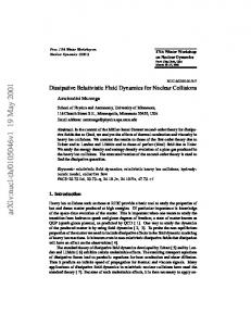
In order to test the validity of RTRFD, we compare it to the solution of the Boltzmann equation, similarly as in Ref. [6]. The numerical method of choice for solving the Boltzmann equation is the Boltzmann approach for multiparton scattering (BAMPS) [11], while the macroscopic field equations are solved using the viscous SHarp And Smooth Transport Algorithm (vSHASTA) [14]. Both fluid dynamics and the Boltzmann equation are solved in Cartesian coordinates with a flat space-time metric g µν = diag(1, −1, −1, −1). We consider a (3+1)–dimensional system, but assume that the matter is homogeneous in the y − z plane, allowing for an inhomogeneous matter distribution only in the longitudinal x–direction. This effectively leads to a (1+1)–dimensional problem. We consider two different initial conditions. In case I, the system is initialized with a homogeneous fugacity, λ0 = eα0 ≡ 1, but with an inhomogeneous pressure profile in the longitudinal direction. In practice we smoothly connect two temperature states T(−∞) = 0.4 GeV and T(+∞) = 0.25 GeV via the Woods-Saxon parametrization with thickness parameter D = 0.3 fm. In case II, the pressure P0 = gT(−∞) 4 /π 2 is homogeneous and the fugacity distribution is also given by a Woods-Saxon profile with D = 0.3 fm, interpolating between λ(−∞) = 1 and λ(+∞) = 0.2. For the degeneracy factor we use g = 16. In both cases, matter is initialized in local thermodynamical equilibrium, i.e., with all dissipative currents (and eigenmodes of the Boltzmann equation) set to zero, and at rest, i.e., with a vanishing collective velocity uµ = 0. These initial conditions are shown in Fig. 1.
p/P0, λ= exp(µ/T)
1.0 0.8
Ι
0.6
ΙΙ
0.4 0.2
p/P0 λ
0.0 -6
-4
-2
0 2 x [fm]
4
6
-6
-4
-2
0 2 x [fm]
4
6
FIG. 1. (Color online) Initial conditions for cases I and II.
In both cases, we consider two exemplary values for the cross section σ = 2 and 8 mb, and consider the solutions after the system has evolved for 6 fm in time. We compare the solution of the Boltzmann equation with that of traditional IS theory [including terms omitted in the original work [3] but quoted in Ref. [15]], as well as with RTRFD at various levels of approximation. Equations (16) contain 13 moments as independent dynamical variables (and 14, if we include bulk viscous pressure). The calculation of the transport coefficients in these equations can be done with increasing accuracy, as more irreducible moments are considered in the expansion (3). The lowest possible accuracy is reached if no more than the original 13 (14) irreducible moments are considered for the calculation of the transport coefficients. At the next level, we include one more set of irreducible moments of tensor-rank one and two (and one more scalar moment in the case of non-vanishing bulk viscous pressure), which leads to a total of 21 (23) irreducible
8 moments. In this way, the number of irreducible moments entering the transport coefficients increases by 8 (9) at each successive level of approximation. For the purpose of this work, we found that going to the third level of iteration, i.e., considering 13 + 8 · 3 = 37 moments (14 + 9 · 3 = 41 in the case of nonvanishing bulk viscous pressure) is sufficient to reach the desired accuracy in the values of the transport coefficients. In the following, we shall compare RTRFD with 13 dynamical degrees of freedom and with the transport coefficients computed with 13 and with 37 moments. We shall term these variants of RTRFD “13/13” and “13/37”. In addition, we also solve Eqs. (25). These contain 21 dynamical degrees of freedom. We compute the corresponding transport coefficients using 37 moments. We shall refer to this variant of RTRFD as “21/37”. In the following figures, the numerical solutions of the Boltzmann equation shall always be displayed by open dots, the results of IS theory by black dash-dotted lines, the solution of RTRFD “13/13” by green dashed lines, that of RTRFD “13/37” by blue dotted lines, and that of RTRFD “21/37” by solid red curves. In order to verify the different fluid-dynamical theories discussed in this paper the solutions of the Boltzmann equation must be calculated to a very high precisison. For this purpose we performed 5 · 104 BAMPS runs and computed the fluid-dynamical quantities as averages over these runs. In Fig. 2 we show the fugacity (top) and thermodynamic pressure (bottom) and in Fig. 3 the heat flow q µ ≡ −(ε + P0 )nµ /n (top) and shear-stress tensor (bottom) for case I. The Boltzmann equation and the fluid-dynamical theories were solved for σ = 2 mb (shown in the left panels of each figure) and for σ = 8 mb (shown in the right panels). For σ = 8 mb, the thermodynamic pressure and shear-stress tensor computed in all fluid-dynamical theories are in good agreement with the numerical solutions of the Boltzmann equation. As we decrease the cross section we expect the agreement between macroscopic and microscopic theory to become worse. This explains why, for σ = 2 mb, the pressure and shear-stress tensor computed within fluid-dynamical theories deviate more strongly from those computed via the microscopic theory. Nevertheless, compared to the fugacity and heat-flow profiles, the agreement is not too bad, even for the smaller value of the cross section. The initial pressure gradient in case I drives, via conservation of momentum, the creation of velocity gradients. On the other hand, the gradient of fugacity is initially zero and turns out to remain small throughout the evolution. In this situation, higher-order terms involving gradients of velocity and of the shear-stress tensor, e.g. κ ¯ 6 ∆µλ ∂ν σ λν ⊂ Kµ and ℓnπ ∆µν ∇λ πνλ ⊂ J µ in the particle diffusion equation (16), become of the same order as the respective (firstorder) Navier-Stokes term κI µ . Therefore, if terms of this type are not properly taken into account, we expect large deviations from the solution of the Boltzmann equation. This can be seen in Figs. 2 and 3 when comparing IS theory, RTRFD “13/13”, as well as RTRFD “13/37” with the Boltzmann result. In all of these variants, the parabolic term ∼ κ ¯ 6 is either absent (IS theory and RTRFD “13/13”) or has to be dismissed (RTRFD “13/37”) for reasons of causality. In addition, IS theory and RTRFD “13/13” do not have the correct value for ℓnπ , because we did not include a sufficiently large number of irreducible moments in its computation. Although RTRFD “13/37” features (within the desired accuracy) the correct value for this transport coefficient (as well as for κ ¯ 6 ), it does even worse in describing the fugacity and heat-flow profiles than the previous two theories. This is because the term ∼ κ ¯ 6 could not be taken into account for reasons of causality, although it is of the same order of magnitude as the term ∼ ℓnπ . These problems of fluid-dynamical theories with only 13 dynamical variables are resolved by RTRFD “21/37” which is the only fluid-dynamical theory considered here that contains all contributions of second-order in the Knudsen number in a hyperbolic fashion. In Fig. 4 we show the fugacity (top) and thermodynamic pressure (bottom) and in Fig. 5 the heat-flow (top) and shear-stress tensor profiles (bottom) for case II. As before, the Boltzmann equation and the fluid-dynamical theories considered were solved for σ = 2 mb (shown in the left panels) and for σ = 8 mb (shown in the right panels). Again, we expect, and see, better agreement between fluid dynamics and the Boltzmann equation for the larger value of the cross section. While the fugacity profiles are in good agreement with the solution of the Boltzmann equation for all fluid-dynamical theories and both values of the cross section, the heat flow is not well described in IS theory and in RTRFD “13/13”: IS theory predicts values for the heat flow which are smaller in magnitude than the Boltzmann equation, while RTRFD “13/13” predicts larger values, even for σ = 8 mb. On the other hand, both RTRFD “13/37” and RTRFD “21/37” describe the heat flow very well or even perfectly, respectively, for both values of the cross section. The reason is that the diffusion coefficient κ has the correct value in these theories (while it deviates by ∼ 30% in both IS theory and RTRFD “13/13”). Since, in case II, the initial pressure gradient is zero and turns out to remain small throughout the evolution, the velocity gradients remain small as well. In this situation, it is important to include higher-order terms that couple the shear-stress tensor to heat flow. This is the reason why the solutions of IS theory and RTRFD “13/13” (where these higher-order terms vanish in the massless limit) are not in good agreement with that of the Boltzmann equation for the thermodynamic pressure and the shear-stress tensor, for both values of the cross section. On the other hand, RTRFD “13/37” does a better job in matching the Boltzmann equation. It is not perfect, because the higher-order terms ∼ η¯5 and ∼ η¯8 were dropped. The best agreement is, again, found within RTRFD “21/37” where all second-order terms in the Knudsen number are taken into account.
9 IS 13/13
1.10
13/37 21/37 BAMPS
1.00
Ι
0.90
σ = 2 mb
σ = 8 mb
λ=exp(-µ/T)
λ=exp(-µ/T)
0.80 1.00 0.80 0.60 0.40
P0/P0(x=-∞)
P0/P0(x=-∞)
0.20 0.00 -6
-4
-2
0 x [fm]
2
4
6
-6
-4
-2
0
2
4
6
x [fm]
FIG. 2. (Color online) Fugacity and thermodynamic pressure profiles at t = 6 fm for case I, for σ = 2 mb (left panels) and σ = 8 mb (right panels) .
Note that, in Fig. 5 the BAMPS results for the shear-stress tensor are strongly fluctuating. This happens because, in this special case, the values of the shear-stress tensor are of the same magnitude as the statistical fluctuations in BAMPS. In order to reduce the statistical fluctuations and to achieve a better resolution, a significantly larger amount of runs would be required.
V.
SUMMARY AND CONCLUSION
In this paper, we compared the equations of motion of RTRFD at various levels of approximation with numerical solutions of the Boltzmann equation for two different types of initial conditons (labeled case I and II). Also, we showed how to use the RTRFD formalism to derive equations of motion that are hyperbolic and, at the same time, include terms up to second order in the Knudsen number. By a careful comparison with numerical solutions of the microscopic theory, we demonstrated that this formalism is able to handle problems with strong initial gradients in pressure or particle number density. The initial conditions, cases I and II, were chosen in such a way that considerably different spatial gradient profiles are generated throughout the fluid-dynamical evolution. In case I, the pressure gradient is initially large which gives rise to large velocity gradients in the later stages of the evolution. This means that, in case I, the shear-stress tensor is mainly generated by its corresponding Navier-Stokes term, i.e., by gradients of velocity. On the other hand, the fugacity gradient is initially zero in case I, and remains relatively small throughout the evolution of the fluid. Therefore, in case I the heat flow is not mainly created by its Navier-Stokes term, i.e., by the gradient of fugacity, but by the coupling term to the shear tensor and shear-stress tensor, i.e., the terms ∆µν ∇λ πνλ and ∆µν ∇λ σνλ in Eqs. (16). Therefore, in this case the higher-order terms in Knudsen number must be included and one really needs to solve the hyperbolic equations derived in this paper to obtain a good agreement. The fact that IS theory is always deviating from the microscopic theory when it concerns heat flow means that it does not predict correctly the terms of order one and two in Knudsen number. On the other hand, in RTRFD “13/37” and RTRFD “21/37” all transport coefficients are computed with a sufficiently large number of irreducible moments. This guarantees that all terms of the desired order are included and is the reason for the better agreement of these fluid-dynamical theories with the microscopic theory. The reason why RTRFD “13/37” fails in certain situations is that important terms have to be neglected in order to preserve hyperbolicity and causality. In case II, the fugacity gradient is initially large while the pressure gradient is zero. This means that the heat flow
10 0.15
IS 13/13 13/37
0.10
21/37 BAMPS
0.05
Ι
0.00 σ = 2 mb
σ = 8 mb
-0.05
(qz/P0)
(qz/P0) × 2
0.20
(π/P0)
(π/P0) × 2
0.15 0.10 0.05 0.00 -0.05 -0.10 -6
-4
-2
0
2
4
6
-6
-4
-2
x [fm]
0
2
4
6
x [fm]
FIG. 3. (Color online) Shear-stress tensor and heat flow profiles at t = 6 fm for case I, for σ = 2 mb (left panels) and σ = 8 mb (right panels).
originates mainly from its Navier-Stokes term while the shear-tress tensor originates mainly from its coupling to heat flow, i.e., the terms ∇ , ∇ , I , and n in Eqs. (16). The fact that the heat flow calculated from IS theory deviates from the solution given by the microscopic theory even in this case, is evidence that the Navier-Stokes term of this theory does not contain the correct transport coefficient. The coupling of the shear-stress tensor with the heat flow in IS theory is also not correctly taken into account. In conclusion, the resummation of irreducible moments for the computation of the transport coefficients was essential to obtain a good agreement with the microscopic theory. It provides not only the correct values for the shear viscosity and heat conduction coefficients, but also for the transport coefficients that couple the respective dissipative currents. Moreover, in situations where higher-order terms are important, one has to make sure to include them in a hyperbolic way, and not simply drop relevant contributions because they are parabolic. These two factors resolved the previously observed differences between the solution of IS theory and of the Boltzmann equation observed in Ref. [6]. As expected, and explicitly demonstrated in this paper, the agreement between solutions of RTRFD and the Boltzmann equation depends on the value of σ. For the cases considered in this paper, we obtained a good agreement for σ = 8 mb, while for σ = 2 mb we started to notice small deviations. In order to improve the agreement for smaller values of the cross section, we would have to include more moments of the Boltzmann equation to describe the state of the system, i.e., such moments would have to contribute not only to the values of the transport coefficients but also as independent dynamical variables. We leave this investigation to future work.
VI.
ACKNOWLEDGEMENTS
The authors thank H. Warringa and J. Noronha for discussions. The work of H.N. was supported by the Extreme Matter Institute (EMMI). E.M is supported by OTKA/NKTH 81655. This work was supported by Helmholtz International Center for FAIR within the framework of the LOEWE program launched by the State of Hesse.
11 IS
1.00
13/13
0.80
BAMPS
13/37 21/37
ΙΙ
0.60 0.40 0.20
σ = 2 mb
σ = 8 mb
λ=exp(-µ/T)
λ=exp(-µ/T)
P0/P0(x=-∞)
P0/P0(x=-∞)
1.02
1.01
1.00
0.99
0.98 -6
-4
-2
0
2
4
6
-6
-4
-2
x [fm]
0
2
4
6
x [fm]
FIG. 4. (Color online) Shear-stress tensor and heat flow at t = 6 fm for case II, for σ = 2 mb (left panels) and σ = 8 mb (right panels).
Appendix A: Transport coefficients
In this appendix we list all transport coefficients of fluid dynamics calculated in this paper. The microscopic formulas for the diffusion and viscosity coefficients, ~κ and ~η, and for the relaxation time matrices, τˆn and τˆπ , are ! ! N1 N2 (1) (2) X X τ0k τ0k (1) (2) ~κ = αk , ~η = αk , (1) (2) τ2k τ1k k=0,6=1 k=0 ! ! N2 N1 (2) (2) (2) (2) (1) (1) (1) (1) X X τ0r λr0 τ0r λr1 τ0r λr0 τ0r λr2 . (A1) , τˆπ = τˆn = (2) (2) (2) (2) (1) (1) (1) (1) τ1r λr0 τ1r λr1 τ2r λr0 τ2r λr2 r=0 r=0,6=1 The transport coefficients of the nonlinear terms in the equation of motion for ~nµ are ! N1 (1) (1) (1) (1) X 1 3τ λ 5τ λ 0r r0 0r r2 δˆnn = , (1) (1) (1) (1) 3 3τ λ 5τ 2r r0 2r λr2 r=0,6=1 ! N1 (1) (1) (1) (1) X 1 τ λ τ λ 0r r0 0r r2 ˆnn = (2r + 3) , (A2) λ (1) (1) (1) (1) 5 τ λ τ 2r r0 2r λr2 r=0,6=1 !# ! N "N (1) (2) (1) (2) 1 2 (1) (2) (2) (1) (2) (2) X 1 X (1 − r) τ0r λr−1,0 (2 − r) τ0r λr−1,1 τ00 F1r λr0 2τ00 F1r λr1 ˆ , (A3) + λnπ = (1) (2) (1) (2) (1) (2) (2) (1) (2) (2) 4 r=0 τ20 (1 − r) τ2r λr−1,0 (2 − r) τ2r λr−1,1 F1r λr0 2τ20 F1r λr1 r=2 "N !# ! N 2 1 (1) (2) (1) (2) (2) X X 0 τ0r λr−1,1 0 τ00 F1r λr1 , (A4) + τˆnπ = −4P0 (1) (2) (2) (1) (2) 0 τ20 F1r λr1 0 τ2r λr−1,1 r=0 r=2 ! ! N ! N1 N2 (1) (2) (1) (2) 1 (1) (2) (2) (1) (2) (2) (1) X X X β λ τ λ τ τ F λ τ F λ τ I 0 0 0r r−1,1 0r r−1,0 00 1r r0 00 1r r1 0r r+2,1 , − + ℓˆnπ = − (1) (2) (1) (2) (1) (2) (2) (1) (2) (2) (1) 4P τ λ τ λ τ F λ τ F λ τ I 0 0 r+2,1 2r r−1,0 2r r−1,1 20 1r r0 20 1r r1 2r r=2 r=0 r=0,6=1 (A5)
12
0.00
ΙΙ
-0.05
IS
σ = 2 mb
(qz/P0)
-0.10
σ = 8 mb
13/13
(qz/P0) × 2
13/37 21/37 BAMPS
0.01
(π/P0) × 5
(π/P0)
0.00
-0.01 -6
-4
-2
0
2
4
6
-6
-4
-2
x [fm]
0
2
4
6
x [fm]
FIG. 5. (Color online) Shear-stress tensor and heat flow profiles at t = 6 fm for case II, for σ = 2 mb (left panels) and σ = 8 mb (right panels).
while those in the equation of motion for ~π µν are N
δˆππ
(2) (2)
2 1X = 3 r=0
N
τˆππ τˆπn
2 2X = (2r + 5) 7 r=0
N2 1 X = 5P0 r=1 N
2 2X ℓˆπn = 5 r=1
ˆπn λ
(2) (2)
4τ0r λr0 (2) (2) 4τ1r λr0
5τ0r λr1 (2) (2) 5τ1r λr1 (2) (2)
τ0r λr0 (2) (2) τ1r λr0
(2) (1)
2τ0r λr+1,0 (2) (1) 2τ1r λr+1,0 (2) (1)
τ0r λr+1,0 (2) (1) τ1r λr+1,0 N
2 1 X =− 10 r=2
!
,
(2) (2)
τ0r λr1 (2) (2) τ1r λr1 (2) (1)
!
3τ0r λr+1,2 (2) (1) 3τ1r λr+1,2 ! (2) (1) τ0r λr+1,2 , (2) (1) τ1r λr+1,2
(2) (1)
(1 + r) τ0r λr+1,0 (2) (1) (1 + r) τ1r λr+1,0
(2)
,
!
(A6)
,
(A7)
(A8) (1)
τ0r (r − 1) λr+1,2 (2) (1) τ1r (r − 1) λr+1,2
!
.
(A9)
[1] W. A. Hiscock and L. Lindblom, Ann. Phys. (N.Y.) 151, 466 (1983); Phys. Rev. D 31, 725 (1985); Phys. Rev. D 35, 3723 (1987); Phys. Lett. A 131, 509 (1988); Phys. Lett. A 131, 509 (1988); G. S. Denicol, T. Kodama, T. Koide, and Ph. Mota, J. Phys. G 35, 115102 (2008); S. Pu, T. Koide, and D. H. Rischke, Phys. Rev. D 81, 114039 (2010). [2] L. D. Landau and E. M. Lifshitz, Fluid Mechanics, (Pergamon; Addison-Wesley, London, U.K.; Reading, U.S.A., 1959). [3] W. Israel and J. M. Stewart, Phys. Lett. 58A, 213 (1976); Ann. Phys. (N.Y.) 118, 341 (1979); Proc. Roy. Soc. London A 365, 43 (1979). [4] P. Huovinen and D. Molnar, Phys.Rev. C79 (2009) 014906. [5] I. Bouras, E. Molnar, H. Niemi, Z. Xu, A. El, O. Fochler, C. Greiner, and D. H. Rischke, Phys. Rev. Lett. 103, 032301 (2009). [6] I. Bouras, E. Molnar, H. Niemi, Z. Xu, A. El, O. Fochler, C. Greiner, and D. H. Rischke, Phys. Rev. C82, 024910 (2010). [7] A. El, Z. Xu, and C. Greiner, Phys. Rev. C 81, 041901 (2010).
13 [8] G. S. Denicol, T. Koide, and D. H. Rischke, Phys. Rev. Lett. 105, 162501 (2010). [9] G. S. Denicol, H. Niemi, E. Molnar, and D. H. Rischke, arXiv:1202.4551 [nucl-th] (to be published in Phys. Rev. D). [10] S. Chapman and T. G. Cowling, The mathematical theory of non-uniform gases, 3rd edition (Cambridge University Press, Cambridge, 1970). [11] Z. Xu and C. Greiner, Phys. Rev. C 71 (2005) 064901; Phys. Rev. C 76, 024911 (2007). [12] S. R. de Groot, W. A. van Leeuwen, and Ch. G. van Weert, Relativistic Kinetic Theory - Principles and applications, North Holland (1980). [13] J. L. Anderson, J. Math. Phys. 15, 1116 (1974); Physica 79A, 569 (1975); Physica 85A, 287 (1976). [14] E. Molnar, H. Niemi, and D. H. Rischke, Eur. Phys. J. C 65, 615 (2010). [15] B. Betz, D. Henkel, and D. H. Rischke, Prog. Part. Nucl. Phys. 62, 556 (2009); B. Betz, D. Henkel, and D. H. Rischke, J. Phys. G G36, 064029 (2009); B. Betz, G. S. Denicol, T. Koide, E. Molnar, H. Niemi, and D. H. Rischke, EPJ Web of Conferences 13, 07005 (2011).