Oct 10, 2006 - practical to require the author to fix the column widths at document authoring time since ... a two stage approach to table layout. In the first stage.
Solving the Simple Continuous Table Layout Problem Nathan Hurst, Kim Marriott, and David Albrecht Clayton School of Information Technology, Monash University Clayton, Victoria, Australia {njh,marriott,dwa}@csse.monash.edu.au
ABSTRACT Automatic table layout is required in web applications. Unfortunately, this is NP-hard for reasonable layout requirements such as minimizing table height for a given width. One approach is to solve a continuous relaxation of the layout problem in which each cell must be large enough to contain the area of its content. The solution to this relaxed problem can then guide the solution to the original problem. We give a simple and efficient algorithm for solving this continuous relaxation for the case that cells do not span multiple columns or rows. The algorithm is not only interesting in its own right but also because it provides insight into the geometry of table layout.
Categories and Subject Descriptors I.7.2 [Document and Text Processing]: Document Preparation—Format and notation, Photocomposition/typesetting
General Terms Algorithms
Keywords automatic table layout,constrained optimization
1.
INTRODUCTION
Tables are provided in virtually all document formatting systems and are one of the most powerful and useful design elements in current web document standards such as (X)HTML, CSS and XSL. In on-line documents it is not practical to require the author to fix the column widths at document authoring time since the table layout needs to adjust to different width viewing environments and to different fonts. Thus, automatic layout of the table is needed. Unfortunately, automatic layout of tables which contain text is not an easy task. Both Wang and Wood [5] and Anderson and Sobti [1] have proven that table layout with
Permission to make digital or hard copies of all or part of this work for personal or classroom use is granted without fee provided that copies are not made or distributed for profit or commercial advantage and that copies bear this notice and the full citation on the first page. To copy otherwise, to republish, to post on servers or to redistribute to lists, requires prior specific permission and/or a fee. DocEng’06, October 10–13, 2006, Amsterdam, The Netherlands. Copyright 2006 ACM 1-59593-515-0/06/0010 ...$5.00.
text is NP-hard. The underlying reason is that if a cell contains text then this implicitly constrains the cell to take one of a discrete number of possible configurations corresponding to different numbers of lines of text. It is not too surprising that it is NP-hard to find which combination of these discrete configurations best satisfies reasonable layout requirements such as minimizing table height for a given width. Hurst, Marriott and Moulder [3] observed that the cell configurations can be approximated by a continuous (nonlinear) constraint that the cell is large enough to contain the area of its textual content. Based on this they suggested a two stage approach to table layout. In the first stage a continuous relaxation of the layout problem is solved in which each cell in the table is required to contain the area of its contents. In the second stage, the solution to the relaxed problem is used to guide the construction of a solution to the original problem. In Hurst et al. [3], it was shown that the continuous table layout problem could be solved in polynomial time using interior point methods to solve conic programming problems [4]. However, interior point solvers for conic programming are quite complex to implement and expensive to buy, relatively slow, and are not incremental. Lack of incrementality means that they are not well-suited to methods such as branch-and-bound in which solutions to many slight variants of the relaxed problem are used to guide the solution to the original problem. For these reasons we have explored other methods for solving the continuous relaxed table layout problem. Here we present a specialised algorithm which is reasonably simple to implement, incremental and considerably faster than conic programming. It also provides insight into the underlying geometry of table optimisation. Our method is a kind of active set method [2]. The only limitation is that it does not directly handle cells that span multiple columns or rows: this is something we are currently addressing.
2.
THE SIMPLE CONTINUOUS TABLE LAYOUT PROBLEM
We assume throughout this paper that the table of interest has n columns and m rows. A layout (w, h) for a table is an assignment of widths, w, to the columns and heights, h, to the rows where wc is the width of column c and hr the height of row r. We restrict attention to simple tables in which each cell in the table is a single grid element (i.e., it spans a single row and column of the table). We let row (d) and col (d), respectively give the row and column of cell d.
We wish to solve a continuous approximation to the original layout problem, called the simple continuous table layout problem (SCTLP), in which rather than requiring a cell to be big enough to contain its textual content we instead require that for each cell d, area(d) ≤ hrow (d) × wcol(d) ,
h1 1 h2 1 h3 1
w1 1 1 1 1/2
w2 1 1 1/2 1/2
w3 4 3 2 4
T1
T2
w1 ↓ & h1 h2 ↓ w2
w3 ↓ h3
where area(d) is the area of the contents of d. In the case of text, this includes the area of the words and a separator between adjacent words. We want to find values for the row Pm heights and column widths such that the table height, r=1 hr , is minimised subject to the cell P containment constraints and the linear constraint 0 ≤ n c=1 wc ≤ W which ensures that the table is no wider than the maximum allowed width, W . An assignment (w, h) to a SCTLP is a feasible solution if it satisfies the constraints, and an optimal solution if it minimises the table height.
(a) Example table and its constraint graph (Table perimeter is 9.0)
Lemma 2.1. Let (w, h) be a feasible solution to a simple continuous table layout problem P that minimizes the table area. For any width W > 0, (αW w, α1W h) is a feasible solution to P which has width W and which minimizes the table height where the scaling factor αW = PnW wi .
(b) Table and constraint graph after rescaling, merging T1 and T2 to obtain constraint graph T3 and then rescaling (Table perimeter is 8.216).
T3
h1 1.225 h2 1.225 h3 1.633
i=1
Lemma 2.2. Let (w, h) be a feasible solution to a simple continuous table layout problem P P that minimizes the total Pn m table perimeter, i.e. minimizes h + w r r=1 c=1 c . Then (w, h) also minimizes table area. Thus, when solving a simple continuous table layout problem, we need only find a feasible solution that minimizes the table’s perimeter: we can then appropriately scale this to find a solution that minimizes the height for a given width.
3.
SOLVING THE SIMPLE CONTINUOUS TABLE LAYOUT PROBLEM
For any feasible solution to a SCTLP that minimizes the table area or perimeter, there must be at least one full cell in each row and each column, where the assignment (w, h) to a SCTLP makes cell d full iff area(d) = hrow (d) × wcol(d) . Since otherwise we could just narrow the row or column and obtain a solution with less area and perimeter. We call a feasible solution with this property reasonable. Consider the table in Figure 1. This shows a reasonable feasible solution to a SCTLP. Each cell contains its area and the table column and rows are annotated with their width or height. The full cells are indicated by an extra border for the cell. The constraints corresponding to the full cells in a SCTLP can be drawn as a constraint graph with nodes for column widths and row heights and an edge for each full cell d between the nodes for hrow (d) and wcol(d) . Figure 1 (a) shows an example table and its constraint graph. This example graph has two important properties: first it is a bipartite graph with row nodes alternating with column nodes on any path; second it is acyclic (in this case with two trees). A key observation behind our algorithm is that any reasonable feasible solution has a corresponding constraint graph with these properties. Consider a single tree T in the constraint graph. It has a single degree of freedom. To see this consider our example. If we scale w1 by s then we must scale h1 and h2 by 1/s and
h1 1.310 h2 1 h3 1.746
w1 0.8165 1 1 1/2
w1 1 1 1 1/2
w2 0.8165 1 1/2 1/2
w2 0.7638 1 1/2 1/2
w1 ↓ & h1 h2 ↓ & w2 w3 ↓ h3
w3 2.450 3 2 4
w3 2.291 3 2 4
h1 ↓ & w2 w3 ↓ h3
w1 ↓ h2
(c) Minimum perimeter layout and the corresponding constraint graph obtained after splitting T3 and rescaling. (Table perimeter is 8.111). Figure 1: Example table and constraint graphs showing how rescaling, merging, then splitting can be used to compute the minimum perimeter layout.
hence w2 by s to ensure that the full cells keep the same area. In general, if we are to preserve the full cells in T we must scale all of the columns in T by the same amount s and all of the rows by 1/s. We wish to minimize the perimeter of the layout. Since the trees are independent we must minimize the perimeter of each tree. Thus we wish to find the column scaling factor s which minimizes X X hr PT = swc + s c∈cols(T )
r∈rows(T )
where cols(T ) is the set of columns in a tree T and rows(T ) the set of rows. Solving dP = 0 we obtain ds sP hr Pr∈rows(T ) s= c∈cols(T ) wc and the optimum layout for the tree is for all c ∈ cols(T ), wc? = swc and for all r ∈ rows(T ), h?r = hr /s. Note that this scales the width and height of the tree so that they become equal, reflecting the fact that the rectangle with the smallest perimeter for a fixed area is a square. The catch is that we may not be able to rescale tree T to its optimal layout since scaling T by s will either narrow columns in T (if s < 1) or narrow rows in T (if s > 1).
Such narrowing may violate the containment constraint for a non-full cell. Thus in the case s < 1 we must compute the smallest safe scaling factor smin the columns can be narrowed by. We need only consider cells d s.t. col (d) ∈ cols(T ) and row (d) 6∈ rows(T ). If smin ≤ s then we can safely rescale T to its optimum value, but if smin > s then we need to make the cell d which gives rise to smin full and merge the tree T with the tree containing row (d). The case when s > 1 is analogous: we simply compute the smallest safe scaling factor smin that the rows of T can be narrowed by. We can repeat this process until each tree is optimally scaled. In the case of our example the tree T1 p is already at its optimal layout since the scaling p factor is 2/2 = 1 while the tree T2 has scaling factor s = 1/4 = 1/2. However the smallest safe scaling factor for T2 is 3/4 reflecting the fact that we can only narrow column 3 to 3 because of the cell (1, 3). Thus we scale T2 by 3/4 and then merge T1 and T2 by making the cell (1, 3) full. We must p now rescale T3 to its optimum value. The scaling factor is (10/3)/5 = 0.8165 giving the table shown in Figure 1(b). Unfortunately, having all trees optimally scaled does not necessarily mean that the global optimum has been reached. By splitting some of the trees and rescaling we may reduce the total table perimeter. For each tree T , we need to check that for each cell d in T that splitting T into two sub-trees by removing d cannot reduce the total table perimeter while still maintaining feasibility. In more detail, let the cell d considered for removal from T occur at row R and column C and call the two sub-trees TR and TC where TR contains row R and TC contains column C. Let P P WR = c∈cols(TR ) wc , HR = r∈rows(TR ) hr , P P WC = c∈cols(TC ) wc , HC = r∈rows(TC ) hr
we find that we can reduce the perimeter by splitting off the sub-tree rooted at h1 . Therefore, we split T3 by removing the edge corresponding to cell (1, 1). This leads to the table layout and constraint graph shown in Figure 1(c). In this case, if the constraint graph is annotated with sub-tree widths and heights then these all satisfy the “no split” conditions so the optimum cannot be improved by splitting any of the trees. Thus we have reached a local minimum and, since the problem is convex (from Lemma 1 [3]), a global optimum. This gives us a simple and very efficient algorithm to solve the SCTLP problem: our implementation is orders of magnitude faster than a general purpose conic programming solver, and takes only a few milliseconds on tables with thousands of elements. First, find an initial reasonable feasible solution. Our implementation chooses the cell with the greatest area in each column to make full for that column. The column width is set to the area of that cell and the row height to 1. Then for each row that does not yet have a full cell, the cell which requires the maximum row height (given the column widths) is made full and the row height set to this value. This was used to find the initial solution in our example (Figure 1(a)). Now we rescale the trees to their optimum size, merging when necessary. Then, we check if a tree needs to split: if it does, we split and rescale and merge as necessary. This is repeated until each tree is at its optimal size and no tree can be split. At this point we have found the layout with the minimum perimeter. Note that this is guaranteed to terminate, as long as there are no redundant constraints, since at each step we reduce the table perimeter. Finally, we scale the table layout to the desired width, giving the layout of minimum height.
Since T is optimally scaled, WR + WC = HR + HC . Thus, there are two possibilities: either (a) HR ≥ WR in which case HC ≤ WC , or (b) HR < WR in which case HC > WC . In case (a), splitting at d and rescaling the two trees will immediately cause the two trees to re-merge since rescaling TR to its optimum will reduce the height of row R and rescaling TC to its optimum will reduce the width of column C, thus reducing the size of d and so violating the constraint. Thus, in this case, the table perimeter cannot be reduced by splitting T at this cell. In case (b), however, splitting at d will allow the perimeter to be reduced while still maintaining feasibility as rescaling TR to its optimum will increase the height of R and rescaling TC to its optimum will increase the width of C, thus increasing the size of d. We can determine in linear time whether any tree needs to be split at a cell by simply traversing the tree bottom-up and computing the difference between the column widths and row heights as we go. More exactly, we assume that our tree has some arbitrary node as root and from this induce a direction to all edges in the tree. At each node k in the tree, we compute Wk the sum of the column widths in the sub-tree rooted at k and Hk the sum of the row heights in the sub-tree rooted at k. If the node k corresponds to a column then we must check that Hk ≤ Wk and if it is a row we must check that Hk ≥ Wk , i.e. case (a) holds. If this is not true then we can improve the optimum by splitting the tree at k. In the case of the example table from Figure 1(b), if we compute the width and height of each node’s sub-tree then
4.
REFERENCES
[1] R. J. Anderson and S. Sobti. The table layout problem. In SCG ’99: Proceedings of the Fifteenth Annual Symposium on Computational Geometry, pages 115–123, New York, NY, USA, 1999. ACM Press. [2] R. Fletcher. Practical Methods of Optimization. John Wiley & Sons, Chichester, New York, Brisbane, Toronto, Singapore, 2nd edition, 2000. [3] N. Hurst, K. Marriott, and P. Moulder. Towards tighter tables. In Proceedings of Document Engineering, 2005, pages 74–83, New York, 2005. ACM. [4] J. Renegar. A Mathematical View of Interior-Point Method in Convex Optimization. SIAM, 2001. [ Edital Universal, 2001 ]. [5] X. Wang and D. Wood. Tabular formatting problems. In PODP ’96: Proceedings of the Third International Workshop on Principles of Document Processing, pages 171–181, London, UK, 1997. Springer-Verlag.