Traditionally robust optimization problems have been solved using an inner-outer ...... Table 5.6: Summary of Results (Example Relevant to Production Systems) ... Mathematical modeling of problems arising in engineering and economics often .... methodology is provided to solve Nash-Cournot energy production games ...
ABSTRACT
Title of Document:
SOLVING TWO-LEVEL OPTIMIZATION PROBLEMS WITH APPLICATIONS TO ROBUST DESIGN AND ENERGY MARKETS Sauleh Ahmad Siddiqui Doctor of Philosophy, 2011
Directed By:
Steven A. Gabriel, Associate Professor Department of Civil and Environmental Engineering Shapour Azarm, Professor Department of Mechanical Engineering
This dissertation provides efficient techniques to solve two-level optimization problems. Three specific types of problems are considered. The first problem is robust optimization, which has direct applications to engineering design. Traditionally robust optimization problems have been solved using an inner-outer structure, which can be computationally expensive. This dissertation provides a method to decompose and solve this two-level structure using a modified Benders decomposition. This gradient-based technique is applicable to robust optimization problems with quasiconvex constraints and provides approximate solutions to problems with nonlinear constraints. The second types of two-level problems considered are mathematical and equilibrium programs with equilibrium constraints. Their two-level structure is simplified using Schur‟s decomposition and reformulation
Form Approved OMB No. 0704-0188
Report Documentation Page
Public reporting burden for the collection of information is estimated to average 1 hour per response, including the time for reviewing instructions, searching existing data sources, gathering and maintaining the data needed, and completing and reviewing the collection of information. Send comments regarding this burden estimate or any other aspect of this collection of information, including suggestions for reducing this burden, to Washington Headquarters Services, Directorate for Information Operations and Reports, 1215 Jefferson Davis Highway, Suite 1204, Arlington VA 22202-4302. Respondents should be aware that notwithstanding any other provision of law, no person shall be subject to a penalty for failing to comply with a collection of information if it does not display a currently valid OMB control number.
1. REPORT DATE
3. DATES COVERED 2. REPORT TYPE
2011
00-00-2011 to 00-00-2011
4. TITLE AND SUBTITLE
5a. CONTRACT NUMBER
Solving Two-Level Optimization Problems With Applications To Robust Design And Energy Markets
5b. GRANT NUMBER 5c. PROGRAM ELEMENT NUMBER
6. AUTHOR(S)
5d. PROJECT NUMBER 5e. TASK NUMBER 5f. WORK UNIT NUMBER
7. PERFORMING ORGANIZATION NAME(S) AND ADDRESS(ES)
8. PERFORMING ORGANIZATION REPORT NUMBER
University of Maryland,College Park,MD, 20782 9. SPONSORING/MONITORING AGENCY NAME(S) AND ADDRESS(ES)
10. SPONSOR/MONITOR’S ACRONYM(S) 11. SPONSOR/MONITOR’S REPORT NUMBER(S)
12. DISTRIBUTION/AVAILABILITY STATEMENT
Approved for public release; distribution unlimited 13. SUPPLEMENTARY NOTES 14. ABSTRACT
15. SUBJECT TERMS 16. SECURITY CLASSIFICATION OF: a. REPORT
b. ABSTRACT
c. THIS PAGE
unclassified
unclassified
unclassified
17. LIMITATION OF ABSTRACT
18. NUMBER OF PAGES
Same as Report (SAR)
222
19a. NAME OF RESPONSIBLE PERSON
Standard Form 298 (Rev. 8-98) Prescribed by ANSI Std Z39-18
schemes for absolute value functions. The resulting formulations are applicable to game theory problems in operations research and economics. The third type of twolevel problem studied is discretely-constrained mixed linear complementarity problems. These are first formulated into a two-level mathematical program with equilibrium constraints and then solved using the aforementioned technique for mathematical and equilibrium programs with equilibrium constraints. The techniques for all three problems help simplify the two-level structure into one level, which helps gain numerical and application insights. The computational effort for solving these problems is greatly reduced using the techniques in this dissertation. Finally, a host of numerical examples are presented to verify the approaches. Diverse applications to economics, operations research, and engineering design motivate the relevance of the novel methods developed in this dissertation.
SOLVING TWO-LEVEL OPTIMIZATION PROBLEMS WITH APPLICATIONS TO ROBUST DESIGN AND ENERGY MARKETS
By Sauleh Ahmad Siddiqui
Dissertation submitted to the Faculty of the Graduate School of the University of Maryland, College Park, in partial fulfillment of the requirements for the degree of Doctor of Philosophy 2011
Advisory Committee: Associate Professor Steven A. Gabriel, Co-Advisor/Chair Professor Shapour Azarm, Co-Advisor Associate Professor Radu V. Balan Professor Dianne P. O‟Leary Professor Lars J. Olson, Dean‟s Representative
© Copyright by Sauleh Ahmad Siddiqui 2011
Acknowledgements First and foremost, I would like to thank my advisers Dr. Steven A. Gabriel and Dr. Shapour Azarm for all their help and support. Their perpetual encouragement, abundant patience, and careful guidance made this work possible. My time at this university was made memorable because of them, and I am proud to look back and realize how much I have learned from them. I would also like to thank my committee members for agreeing to advise me on this work: Dr. Radu V. Balan, for overlooking the mathematical aspects in both my preliminary oral exam and dissertation; Dr. Dianne P. O‟Leary, whose survival manual for graduate study in the computer and mathematical sciences provided valuable advice; and Dr. Lars J. Olson for graciously agreeing to serve as the Dean‟s representative. I am grateful that they have taken time out from their busy schedules to provide insight. I also want to acknowledge funding received from the Office of Naval Research and the Norwegian Research Council. The work presented in this dissertation was supported in part by the Office of Naval Research Contract N000140810384. The LinkS project funded by Norwegian Research Council via the Norwegian University of Science and Technology and SINTEF (UMD Award number 013768-001) also supported part of the work in this dissertation. Such support does not constitute an endorsement by the funding agency of the opinions expressed in this dissertation.
ii
Table of Contents ACKNOWLEDGEMENTS ....................................................................................... ii TABLE OF CONTENTS .......................................................................................... iii LIST OF TABLES ..................................................................................................... vi LIST OF FIGURES .................................................................................................. vii NOMENCLATURE AND ABBREVIATIONS .................................................... viii CHAPTER 1: INTRODUCTION .............................................................................. 1 1.1. MOTIVATION AND OBJECTIVE .................................................................. 1 1.2. RESEARCH COMPONENTS........................................................................... 3 1.2.1. Solving Robust Optimization Problems...................................................... 3 1.2.2. Solving Mathematical Programs and Equilibrium Problems with Equilibrium Constraints ........................................................................................ 4 1.2.3. Solving Discretely-Constrained Mixed-Integer Linear Complementarity Problems ............................................................................................................... 4 1.3. ORGANIZATION OF DISSERTATION ......................................................... 5 CHAPTER 2: DEFINITIONS AND LITERATURE REVIEW ............................ 7 2.1. INTRODUCTION ............................................................................................. 7 2.2. DEFINITIONS AND TERMINOLOGIES........................................................ 7 2.2.1. Robust Optimization ................................................................................... 9 2.2.2. Mathematical and Equilibrium Programs with Equilibrium Constraints . 12 2.2.3 Discretely-Constrained Mixed Linear Complementarity Problems .......... 16 2.3. OVERVIEW OF PREVIOUS WORK ............................................................ 19 2.3.1 Robust Optimization .................................................................................. 19 2.3.3 Mathematical and Equilibrium Programs with Equilibrium Constraints .. 23 2.3.4. Discretely-Constrained Mixed Linear Complementarity Problems ......... 24 2.4. PRELIMINARIES ........................................................................................... 27 2.4.1. Benders Decomposition ............................................................................ 27 2.4.2. Disjunctive Constraints ............................................................................. 30 2.4.3. Approximating Nonlinear Functions using SOS Type 1 and Type 2 Variables ............................................................................................................. 31 CHAPTER 3: SOLVING ROBUST OPTIMIZATION PROBLEMS USING A MODIFIED BENDERS METHOD ........................................................................ 36 3.1. INTRODUCTION ........................................................................................... 36 3.2. INTERVAL UNCERTAINTY ........................................................................ 37 3.3 MODIFIED BENDERS DECOMPOSITION .................................................. 54 3.3.1. Formulation of Approach: Solving Robust Linear Programs ................... 54 3.3.2. Formulation of Approach: Solving Robust Optimization Problems with Quasiconvex Constraints .................................................................................... 59 3.3.3. Formulation of Approach: Solving Robust Optimization Problems with Nonlinear Constraints ......................................................................................... 63 3.4. NUMERICAL RESULTS ............................................................................... 69 3.4.1. Numerical Example (Example 1) to Show Methodology Step-by-Step ... 70 3.4.2. Numerical Results ..................................................................................... 74 iii
3.5. ENGINEERING DESIGN AND OTHER APPLICATIONS ......................... 76 3.5.1. Fleury‟s Weight Minimization .................................................................. 76 3.5.2. Design of a Welded Beam ........................................................................ 77 3.5.3. Heat Exchanger Design............................................................................. 81 3.5.4. Building Energy Intensive Infrastructure.................................................. 87 3.6. SUMMARY ..................................................................................................... 90 CHAPTER 4: SOLVING MATHEMATICAL PROGRAMS AND EQUILIBRIUM PROGRAMS WITH EQUILIBRIUM CONSTRAINTS ........ 91 4.1. INTRODUCTION ........................................................................................... 91 4.2. SOLVING MATHEMATICAL PROGRAMS WITH EQUILIBRIUM CONSTRAINTS ..................................................................................................... 92 4.2.1. Changing the Formulation of the Lower-Level Problem .......................... 92 4.2.2. Approximating The Absolute Value Function Using Special Ordered Sets of Type 1 Variables ............................................................................................. 95 4.2.3. Approximating Absolute Value Function Using a Penalty Method ......... 97 4.2.4. Algorithm 1 to Solve Mathematical Programs with Equilibrium Constraints ........................................................................................................ 100 4.2.5. Numerical Results ................................................................................... 101 4.3. SOLVING EQUILIBRIUM PROGRAMS WITH EQUILIBRIUM CONSTRAINTS ................................................................................................... 112 4.3.1. Extending Algorithm 4.1 to Equilibrium Programs with Equilibrium Constraints ........................................................................................................ 112 4.3.2. Algorithm 4.2 to Solve Equilibrium Problems with Equilibrium Constraints (Heuristic) ...................................................................................... 114 4.3.3. Numerical Results for Equilibrium Programs with Equilibrium Constraints ........................................................................................................................... 115 4.4. THE NORTH AMERICAN GAS MODEL .................................................. 120 4.4.1. Introduction ............................................................................................. 120 4.4.2. Shale Gas in the United States ................................................................ 122 4.4.3. Scenario Results ...................................................................................... 126 4.5. SUMMARY ................................................................................................... 134 CHAPTER 5: SOLVING DISCRETELY-CONSTRAINED MIXED LINEAR COMPLEMENTARITY PROBLEMS ................................................................. 135 5.1. INTRODUCTION ......................................................................................... 135 5.2. DISCRETELY-CONSTRAINED MIXED LINEAR COMPLEMENTARITY PROBLEMS ......................................................................................................... 137 5.2.1 Epsilon-Integrality ................................................................................... 137 5.2.2. Sigma-Complementarity ......................................................................... 139 5.2.3. Complementarity, Integrality Trade-off.................................................. 140 5.2.4. Formulation to Solve Discretely-Constrained Mixed Linear Complementary problems ................................................................................. 142 5.3. DISCRETELY-CONSTRAINED NASH-COURNOT GAMES .................. 144 5.3.1. Formulation of a DC-Nash game by Gabriel et al. (2011b) ................... 145 5.3.2. First Numerical Example ........................................................................ 153 5.3.3. Results for First Numerical Example ...................................................... 157 5.3.4. Numerical Example Relevant to Production Systems ............................ 160
iv
5.4. DISCRETELY-CONSTRAINED NETWORK PROBLEMS ...................... 163 5.4.1. First Network Example ........................................................................... 164 5.4.2. Second Network Example....................................................................... 169 5.5. SUMMARY ................................................................................................... 179 CHAPTER 6: CONCLUSIONS ........................................................................... 181 6.1. CONCLUDING REMARKS ......................................................................... 181 6.1.1. Robust Optimization ............................................................................... 181 6.1.2. MPECs and EPECs ................................................................................. 183 6.1.3. Discretely-Constrained Mixed Linear Complementarity Problems ....... 184 6.2. MAIN CONTRIBUTIONS ............................................................................ 185 6.3. FUTURE RESEARCH .................................................................................. 187 6.3.1. Multiobjective Mixed-Integer Robust Optimization .............................. 187 6.3.2. Solving Nonlinear MPECs and EPECs................................................... 188 6.3.3. Solving Large-Scale Mixed-Integer Complementary Problems ............. 189 APPENDICES ......................................................................................................... 190 APPENDIX A: ROBUST OPTIMIZATION TEST PROBLEMS ....................... 190 APPENDIX B: DISCUSSION ON FUNCTION CALLS .................................... 198 BIBLIOGRAPHY ................................................................................................... 201
v
List of Tables Table 2.1: Definition of Terms for Robust Optimization Table 2.2: Definition of Terms for Benders Decomposition Table 3.1: Analysis of function calls for one iteration Table 3.2: Solution Steps for Modified Benders Approach Table 3.3: Detailed Solution for Simple Problem Table 3.4: Description of Test Problems Table 3.5: Results for Fleury‟s Weight Minimization Like Problem Table 3.6: Results of Welded Beam Example Table 3.7: Design Variables and Parameters with Uncertainty Table 3.8: Results for Heat Exchanger Design Table 3.9: Number of Iterations and CPU Time to Solve Problems Table 3.10: Results for Increasing Uncertainty in t2 Table 4.1: Definition of terms for simple example Table 4.2: Different Datasets to Compare (4.13), (4.15), and (4.16) Table 4.3: Different Cases to Compare Solutions to (25) Table 4.4: Results for Dataset 1 Table 4.5: Results for Dataset 2 Table 4.6: Results for Dataset 3 Table 4.7: Results for Dataset 1 Table 4.8: Results for Dataset 2 Table 4.9: Results for Dataset 3 Table 4.10: World Gas Model Nodes: Coverage of States and Shale Basins Table 4.11: Prices in $/MMBTU in 2025 Table 5.1: Bimatrix Nash-Cournot Game, Profits(q1/q2) Table 5.2: Nash-Cournot Game, Profits(q1/q2), (Only Adjustments a=9, ρ₂ = 3) Table 5.3: Description of Formulation Variations Table 5.4: Summary of Results (a = 9, b = 1, β₁= β₂ = 1,ρ₁ = 1, ρ₂ = 3) Table 5.5: Summary of Results (a = 9, b = 1, β₁= β₂ = 1,ρ₁ = 1, ρ₂ = 3) Table 5.6: Summary of Results (Example Relevant to Production Systems) Table 5.7: Summary of Results (Example Relevant to Production Systems) Table 5.8: Parameter Values Used in First Network Example Table 5.9: Description of Formulation Variations Table 5.10: Solution to Power Market Example Table 5.11: Dataset Used in Second Network Example Table 5.12: Description of Formulation Variations for Second Network Example Table 5.13: Results for Second Network Problem (Integer Variables) Table 5.14: Results for Second Network Problem (Other Variables)
vi
List of Figures Figure 1.1: Organization of Dissertation Figure 2.1: The Structure of a Two-Level Problem Figure 2.2: Representation of a Robust Optimization Problem Figure 2.3: Representation of an MPEC Figure 2.4: Representation of an EPEC Figure 2.5: Representation of a DC-MLCP Figure 2.6: Approximating a Nonlinear Function Using SOS Type 1 Variable Figure 2.7: Approximation of Nonlinear Functions using SOS Type 2 Variables Figure 3.1: Comparison of the Feasible Region with the Robust Feasible Region Figure 3.2: The Robust Benders Cuts to Estimate the Maximum Endpoint of αu Figure 3.3: Checking Feasibility by Interval-Optimal Points for Constraints Figure 3.4: Adding a modified (Robust) Benders Cut Figure 3.5: Design of a Welded Beam (Gunawan & Azarm, 2004) Figure 3.6: Heat Exchanger Schematic Figure 4.1: Computational Time for Solving Problem Figure 4.2: A Marginal Cost Structure for Shale Gas (Skagen, 2010) Figure 4.3: A Marginal Cost Structure for Shale Gas Figure 4.4: Overall Production in 2025 as Predicted by the Model Figure 4.5: Producer Profit in 2025 as Predicted by the Model Figure 4.6: Shale Producers in 2025 as Predicted by the Model Figure 4.7: Consumption in 2025 as Predicted by the Model Figure 5.1: The Tradeoff Between Complementary and Integrality Figure 5.2: Computational Time for First Numerical Example Figure 5.3: Computational Time for Example Relevant to Production Systems Figure 5.4: Diagram of First Network Example Figure 5.5: Representation of Second Network Example
vii
Nomenclature and Abbreviations BCM
Billion Cubic Meters
DC-MLCP Discretely-Constrained Mixed Linear Complementary Problems DC-Nash
Discretely-Constrained Nash Game
EPEC
Equilibrium Program with Equilibrium Constraints
f
Objective Function (Unless stated otherwise)
g
Inequality Constraint Function (Unless stated otherwise)
KKT
Karush-Kuhn-Tucker Conditions
LBF
Pound Force
LP
Linear Program
MCF
Million Cubic Feet
MIP
Mixed Integer Program
MILP
Mixed Integer Linear Program
MMBTU
One million British Thermal Units; measurement of heat energy
MPEC
Mathematical Programs with Equilibrium Constraints
NCP
Nonlinear Complementary Problem
The real numbers
SOS
Special Ordered Set
x
Decision Variable
WGM
World Gas Model
Z
The Integers
viii
Chapter 1: Introduction 1.1. Motivation and Objective Mathematical modeling of problems arising in engineering and economics often requires formulations where optimal decisions need to be made at two different levels. These levels can be distinguished by time, space, decision choices, or even sets of players. An optimal decision at each level, we assume, can be obtained using an optimization problem. Consider some of many types of decisions made by the computer processor manufacturer Intel. First while making the processor, manufacturing errors and uncertainty can lead to their “best” design being infeasible. If not infeasible, the design might not be the best choice under uncertainty. This decision needs to be made accounting for the uncertainty or errors that can develop after manufacturing the product. Second, while deciding the price (or quantity) of the processor, Intel would have to take into account what its competitors are doing and if the government has made any regulations regarding taxation or distribution. Setting a price, thus, not only depends on Intel‟s own costs but the strategy of other actors at a different level than Intel. Finally, Intel needs to decide the number of processors to ship to specific locations. Even considering a simplified version of the market makes this a complex problem as network dynamics, transportation costs, and local demand all weigh into the decision. But, more importantly, the processors can only be transported in positive integer number quantities, as opposed to fractional quantities.
1
All the problems classified above fall under the umbrella of two-level problems. The first decision, regarding uncertainty, requires the initial proposed design of the chip to be such that the presence of uncertainty does not cause the design to be infeasible and/or suboptimal. The decision is thus made to ensure feasibility of design constraints as well as minimum variation in a design‟s performance under uncertainty. Such a problem will be described in this dissertation as a Robust Optimization problem. The second type of problem about making a profit-maximizing decision with other players present in a non-cooperative competitive environment is known as a Stackelberg Game in economics and falls under the broad heading of Mathematical Programs with Equilibrium Constraints or MPECs. These problems have a wide variety of applications, and in their general form can encompass robust optimization problems as well. A special class of MPECs with certain mathematical properties will be considered in this dissertation along with their extension to Equilibrium Programs with Equilibrium Constraints or EPECs. The third problem is about solving non-cooperative games as well, except the decision at the second level is to make sure that the choice made is integer rather than continuous. This is more of a computational issue, but nevertheless the techniques to solve such problems have important applications. These problems fall into the class of Discretely-Constrained Mixed Linear Complementarity Problems or (DC-MLCPs). The two levels are a common feature to all these problems, and the biggest challenge to overcome this two-level structure is computational time. A nested structure causes a large increase in computational effort with an increase in variables
2
and/or decision space (Bialas & Karwan, 1982). The focus of this dissertation is on developing decomposition based solution techniques that reduce computational effort significantly for these three types of problems. These new techniques will then be implemented on a variety of examples from engineering and energy markets.
1.2. Research Components 1.2.1. Solving Robust Optimization Problems The goal of robust optimization problems is to find an optimal solution that is minimally sensitive to uncertain factors. Uncertain factors can include inputs to the problem such as parameters, decision variables, or both. Given any combination of possible uncertain factors, a solution is said to be robust if it is feasible and the variation in its objective function value is acceptable within a given user-specified range. Previous approaches for general nonlinear robust optimization problems under interval uncertainty involve nested optimization and are not computationally tractable. The overall objective in this dissertation is to develop an original and efficient robust optimization method that is scalable and does not contain nested optimization.
The proposed method is applied to a variety of numerical and
engineering examples to test its applicability. Current results show that the approach is able to numerically obtain a locally optimal robust solution to problems with quasiconvex constraints (≤ type) and an approximate locally optimal robust solution to general nonlinear optimization problems. A portion of this research component has been presented in (Siddiqui et al., 2011a) and (Siddiqui et al., 2011c).
3
1.2.2. Solving Mathematical Programs and Equilibrium Problems with Equilibrium Constraints This dissertation presents an original method for solving mathematical programs and equilibrium problems with equilibrium constraints (MPECs and EPECs). Schur‟s decomposition followed by two separate methods of approximating absolute-value functions are presented and used to solve large-scale MPECs. The advantage of this method over traditional methods for solving MPECs is that computational time is much lower, which is corroborated by numerical examples. An extension to solve EPECs is also presented, along with a small numerical example. Finally, an application of the method to an MPEC representing the United States natural gas market is given. A portion of this research component has been presented in (Siddiqui & Gabriel, 2011b) and (Gabriel et al., 2011c). 1.2.3. Solving Discretely-Constrained Mixed-Integer Linear Complementarity Problems This research thrust presents an original modification to a recent approach for solving discretely-constrained, mixed linear complementarity problems (DC-MLCPs). Such formulations include a variety of interesting and realistic models of which discretelyconstrained Nash games and network equilibrium problems are considered. A methodology is provided to solve Nash-Cournot energy production games allowing some variables to be discrete. Normally, these games can be stated as mixed complementarity problems but only permit continuous variables in order to make use of each producer's Karush-Kuhn-Tucker conditions. The proposed approach allows for more realistic modeling and a compromise between integrality and 4
complementarity to avoid infeasible situations. A mixed-integer, linear program formulation is used to solve the DC-MLCP in which both complementarity as well as integrality are allowed to be relaxed. A portion of this research component has been presented in (Gabriel et al., 2011a) and (Gabriel et al., 2011b).
1.3. Organization of Dissertation The remainder of this dissertation is organized as follows. Chapter 2 provides background and a thorough literature review for the three proposed research components. Chapter 3 provides the proposed solution methodology for robust optimization problems. The chapter also provides several engineering applications as well as numerical examples. The chapter is concluded by an example of an application to a carbon emissions related problem. Chapter 4 provides details on the algorithm used to solve MPECs and EPECs as well as computational issues. The chapter also provides numerical examples to corroborate these approaches, as well as an application to the North American natural gas market. Chapter 5 provides the proposed solution technique for discretely-constrained mixed linear complementary problems with examples of discretely-constrained Nash games and energy networks. Chapter 6 provides conclusions and directions for future research. Figure 1.1 displays the organization of this dissertation. Note that the dashed line shows that a technique developed in Chapter 4 will be used in Chapter 5.
5
Chapter 1: Introduction
Chapter 2: Background
Chapter 3: Robust Optimization
Chapter 4: MPECs and EPECs
Chapter 6: Conclusions
Figure 1.1: Organization of Dissertation
6
Chapter 5: DC-MLCPs
Chapter 2: Definitions and Literature Review 2.1. Introduction This chapter will provide the necessary background for two-level optimization problems including definitions, terminologies, and a thorough literature review. This chapter will initially give mathematical definitions of two-level problems, and explain how robust optimization, MPECs and EPECs, and DC-MLCPs can all be cast as twolevel problems. While two-level problems can be shown to have a general formulation, each of the three different types considered in this dissertation need different treatment to come up with the most efficient solution. Although solving all three efficiently will involve the use of decomposition techniques, many other alternatives exist in the literature which will also be discussed. Finally, some preliminary mathematical ideas and traditional algorithms will also be introduced. This chapter first goes through the definition and terminologies used in this dissertation. In particular, the next section defines each of the three two-level problems considered along with other definitions. A literature review is provided next followed by two preliminary topics.
2.2. Definitions and Terminologies In general, the two-level optimization problems considered in this dissertation can be expressed as the following
7
min f ( x u , x l )
(2.1)
s.t. ( x u , x l ) xl S (xu )
where the continuous variables x u nu , x l nl are, respectively, the vector of upper-level, lower-level variables, f ( x u , x l ) is the upper level objective function1, is the joint feasible region between these sets of variables and S ( x u ) is the solution set of the lower-level problem that can be an optimization problem, a nonlinear complementarity problem (NCP) (Cottle et al., 2009), or a variational inequality problem (VI)
(Faccinei & Pang, 2003).
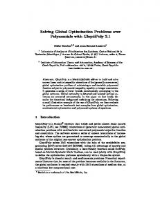
Figure 2.1 shows a diagrammatic
representation of a two-level problem where the nested structure is revealed.
minimize f(xu,xl) (Upper-Level Problem)
xu
xl
Consider xu and calculate xl ( x ufixed , x l ) (Lower-Level Problem)
Figure 2.1: The Structure of a Two-Level Problem
1
Note that when solving EPECs, several such two-level problems will be solved.
8
2.2.1. Robust Optimization Table 2.1 describes the terminology used for robust optimization. Table 2.1: Definition of Terms for Robust Optimization Symbol
Interpretation
x
Vector of decision variables
f
Objective function to be minimized
g j ( x, xˆ )
Constraint functions of the form “≤ 0”
x
Maximum deviations of uncertain variables from nominal values
xˆ
Deviations from nominal values of uncertain variables and parameters, respectively: xˆ x,x
f 0
User-specified tolerance for acceptable variation in objective function under uncertainty
The goal in robust optimization is to optimize the objective function with respect to uncertain decision variables x, satisfying all constraints and ensuring the objective function variation is kept within an acceptable range f 0 , while accounting for uncertainty in decision variables. Specifically, this dissertation considers robust optimization problems of the form2:
2
Note that equality constraints are considered to be formulated as two inequality constraints in
formulation (2.2). Alternatively one can explore the approach for robust optimization with equality constraints (Rangavajhala et al., 2007) but that has not been explored in this dissertation.
9
min f ( x, xˆ ) x
s.t. f ( x, xˆ ) f ( x,0) 1 f 0 g j ( x, xˆ ) 0 j 1,.., J
(2.2)
x R n , xˆ R nu xˆ [x, x] where f and g are continuously differentiable in both x and xˆ . Figure 2.2 diagrammatically shows the structure of a robust optimization problem.
minimize f(x) (Objective Function)
xˆ
x
Check Constraint Violation under Uncertainty ( x fixed , xˆ )
(Constraints Violated under Uncertainty?)
Figure 2.2: Representation of a Robust Optimization Problem
In the next few paragraphs, terms used in this dissertation are defined.
Definition 2.1: Quasiconvex Function: A function g ( x, xˆ ) is said to be quasiconvex in xˆ x,x if for all xˆ x,x , g ( x, xˆ) maxg ( x, x), g ( x,x) for all x (Bazaraa et al., 1993). 10
Definition 2.2: Objective robustness: For a candidate point xc objective robustness holds if inequality f ( x c , xˆ ) f ( x c ,0) 1 f 0
(2.3)
is satisfied for all xˆ x, x.
Thus, this inequality ensures that the maximum objective function variation stays below a certain predetermined maximal amount f 0 when presented with deviations in uncertain variables and parameters.
Definition 2.3: Feasibility robustness: For a candidate solution xc if
g j ( x c , xˆ ) 0
j 1,..., J
(2.4)
is satisfied for all xˆ x, x then feasibility robustness holds.
Note that equation (2.3) is just another constraint, so it can be easily incorporated into inequality (2.4) when stating a general formulation that only includes feasibility robustness. From this point on, inequality (2.3) will not be stated separately in any formulation but will be assumed to be incorporated in inequality (2.4). For a more detailed description on objective robustness, please refer to (Li et al., 2006).
Definition 2.4: Robust point: A robust point is both objectively and feasibly robust. 11
Definition 2.5: Locally optimal robust: For a robust optimization problem, a locally optimal robust solution x*, is a robust point such that there exists a neighboring set U of robust solutions for which x* is optimal ( f ( x*) f ( x), x U ).
It is essential that the neighboring set be made up of only robust points otherwise the term is ill-defined. There is also a global counterpart as defined below.
Definition 2.6: Globally optimal robust: For a robust optimization problem, a globally optimal robust solution x*, is a robust point such that x* is optimal ( f ( x*) f ( x), x ) in the feasible region.
2.2.2. Mathematical and Equilibrium Programs with Equilibrium Constraints In general, a mathematical program with equilibrium constraints is given by 3
min f ( x, y ) s.t. ( x, y )
(2.5)
y S ( x) n
where the continuous variables x nx , y y are, respectively, the vector of upper-level, lower-level variables,
3
f (x,y) is the upper-level single-objective
Without loss of generality, we assume that the variables x and y are nonnegative, which is
incorporated in the decision space Ω.
12
function, is the joint feasible region between these sets of variables and S(x) is the solution set of the lower-level problem that can be an optimization problem, a
problem (Luo et nonlinear complementarity problem (NCP), or variational inequality al., 1996). One focus of this dissertation is when S(x) is a solution to a nonlinear complementarity
problem.
Having
a
function g : n n ,
a
nonlinear
complementarity problem is to find a vector z n such that:
z0 T
g ( z ) 0
(2.6)
z g ( z) 0
If S(x) is the solution set of an NCP, (2.5) can be rewritten as
min f ( x, y ) s.t. ( x, y ) y0 g ( x, y ) 0
(2.7)
y T g ( x, y ) 0 n
where g ( x, y) : nx y
ny
is a vector-valued function.
Similarly, an EPEC is defined as a game between N players at the top level where each top-level player solves an optimization problem of the form (2.7). Hence, an EPEC with a common lower-level for each of the N upper-level players typical of Stackelberg leaders in energy production with the rest of the market represented by the lower-level problem is given by
13
min f j ( x, y )
j 1,..., N
s.t. ( x, y ) y0 g ( x, y ) 0
(2.8)
y T g ( x, y ) 0 Figure 2.3 shows the diagrammatic representation4 for an MPEC and Figure 2.4 shows the diagrammatic representation for an EPEC.
4
Nash-Cournot in this diagram implies that an individual player solves their own optimization problem
with other players‟ decisions being fixed.
14
maximize Profit(x,y) (Decides the value of x)
x
y
Nash-Cournot (xfixed, y)
(Take x fixed and solve for y) Figure 2.3: Representation of an MPEC
Nash-Cournot (x, yfixed)
(Decides the value of x)
x
y
Nash-Cournot (xfixed, y)
(Observe x and solve for y) Figure 2.4: Representation of an EPEC 15
2.2.3 Discretely-Constrained Mixed Linear Complementarity Problems It is not immediately obvious why the problem considered in this subsection is a twolevel problem. The problem in its original form is not, but it needs to be converted into a two-level form for the particular solution technique (Gabriel et al., 2011a; Gabriel et al., 2011b) to be applicable. In general, a discretely-constrained mixed linear complementarity problem is given as follows: given the vector q (q1 , q2 )T
A and matrix A 11 A21
A12 , find z ( z1 , z2 )T n1 n2 such that 5 A22 0 q1 A11 0 q2 A21
z A12 1 z1 0 z2 z A22 1 z 2 , z 2 free z2
(2.9)
z1 c , c C1 , z1 d Z , d D1 z2 c , c C2 , z2 d Z , d D2 The indices for zi, i = 1, 2 are partitioned into continuous-valued (denoted by the set Ci) and discrete-valued variables (denoted by the set Di), i.e.,
zi zi Ci , zi Di , i 1,2 with the continuous variables shown first without loss of T
T
T
generality. From here on, unless otherwise indicated, the discrete sets,
D1 0,1,..., N and D2 N1 ,...,1,0,1,..., N 2 will be assumed with N, N1, N2, nonnegative integers.
5
Here the superscript T denotes the transpose function. The symbol
means that the product of the two terms must be zero.
16
denotes complementary which
Finding a solution to this DC-MLCP can be thought of as a two-level problem, even though (2.9) formulates it in one level. The upper level minimizes deviations from an integer solution and complementary, i.e., ensures that as close as possible to an integer solution is obtained while satisfying complementary conditions with a minimum deviation as well, while the lower level solves a complementary problem assuming some deviation from integers has been fixed at the upper level. Figure 2.5 shows the diagrammatic representation of a discretely-constrained mixed linear complementary problem, while the following formulation describes the twolevel formulation. Note that the first two inequality constraints and the first equality constraint (the first three constraints) form a complementary problem. Hence, the two-level structure6 is apparent in the following formulation. Chapter 5 will describe in detail how this two-level formulation is obtained.
6
Compare (2.10) to (2.1). The upper-level variables are ε and ζ, i.e., x u and the first three lines
in (2.10) define the upper-level problem. The lower level variables z, have x l z1 and are part of z 2 the solution set of the discretely-constrained complementary problem given by the last four lines of (2.10).
17
min 1T 1T
s.t. 1 , d D1 D2 2 d c , c C1
d
q1 A11
z A12 1 z1 0 z2
z A22 1 z 2 , z 2 free z2 z1 c , c C1 , z1 d 1 d Z , d D1 0 q 2 A21
z 2 c , c C 2 , z 2 d 2 d Z , d D2
18
(2.10)
minimize f (ε,ζ,z) (Minimize deviations ε,ζ)
ε,ζ
z
Complementary Problem (εfixed , ζ fixed , z)
(Observe ε,ζ and solve for z)
Figure 2.5: Representation of a Discretely-Constrained Mixed Linear Complementary Problem
2.3. Overview of Previous Work 2.3.1 Robust Optimization This dissertation‟s approach for solving robust optimization problems (hereafter referred to as the modified Benders method), which will be described in Chapter 3, will now be compared to previous methods. A comprehensive review of the literature was conducted and the main distinctions between the proposed modified Benders method and previous works are presented as follows. The robust optimization problems in the proposed modified Benders method also involve nonlinear (for example, Welded Beam and Heat Exchanger, which both
19
involved nonconvex constraint functions) constraint functions7. This is more general than only considering linear constraint functions in the problem as reported in the literature (e.g., Balling et al., 1986; Ben-Tal & Nemirovski, 2002; Bertsimas & Sim, 2006; Soyster, 1973) or quadratic (e.g., Li et al., 2011) as well as other versions involving convex programs (e.g., Ganzerli & Pantelides, 1999) or linearization to solve the problem (e.g., Balling et al., 1986). The modified Benders method is able to obtain exact locally optimal robust solutions to problems with quasiconvex constraints as well as non-convex quadratic programs, which no one method in the reported literature is able to achieve. Other approaches also consider distributions for uncertainty (e.g., Lee et al., 2009; Lagaros & Papadrakakis, 2007) while the approach of this dissertation looks at a worst-case analysis for interval uncertainty8 without any explicit probability distribution or a nested optimization structure. Moreover, the modified Benders method is able to handle large uncertainties which earlier methods
7
In some cases, although not considered in this dissertation, a slightly stricter condition with convexity
in the lower-level of the Benders decomposition method is needed. However, we did not encounter this in any of our test problems. A workaround to this problem is available in (Gabriel et al., 2010). This involves sampling the domain of the objective function of the lower-level optimization problem to determine the convex portions of this function. This numerical approximation scheme can be applied to the modified Benders method to determine convexity of the objective function of the lower-level optimization problem. 8
Note that this dissertation considers robust optimization problems with interval uncertainty, while
there is a substantive amount of literature considering other types of uncertainty. Refer to (Bertsimas & Sim, 2006; (Ben-Tal et al., 2009).
20
(e.g., Balling et al., 1986; Soyster, 1973; Ganzerli & Pantelides, 1999) were not able to tackle. The proposed approach preserves the computational tractability, theoretically and practically, of the deterministic (i.e., nominal) problems. By contrast, under interval uncertainty, the computational effort for previous methods (e.g., Gunawan & Azarm, 2004; Li et al., 2006) to obtain robust solutions is much higher than their deterministic counterparts. However, results from a variety of numerical experiments show that the computational effort of solving the robust optimization problems is not much greater than that of their deterministic counterparts for the modified Benders method. Moreover, the modified Benders method is scalable, in that by numerical tests, the number of function calls per iteration increases at most linearly (numerical result) with an increase in the number of variables, uncertainty variables, and constraints. Since this dissertation‟s approach is based on gradient-based methods, a globally optimal robust solution can never be guaranteed for the complete class of continuous, non-convex problems. However, this dissertation uses the idea of a locally optimal robust solution, and shows that this approach can obtain a locally optimal robust solution for nonlinear robust optimization problems. In addition to the uncertainty in the data of the problems (i.e., the parameters), interval uncertainty is considered in the decision variables corresponding to manufacturing tolerances, implementation errors, etc. where optimized values cannot be achieved exactly, which is very common in practical engineering applications. For the current robust optimization formulations in the literature (e.g., Ben-Tal &
21
Nemirovski, 2008; Lu et al., 2010; Qiu & Wang, 2010; Zhu & Ting, 2001), considering uncertainty in the decision variables may considerably change those formulations or increase the complexity of the problem. The approach in this dissertation, however, keeps the same formulation and obtains locally optimal robust solutions to these problems with not much greater computational effort than the deterministic problem. There has been an abundance of literature modifying Benders decomposition method (Benders, 1962) to solve various types of optimization problems. However, to my knowledge, there have not been any modifications to Benders method that solve nonlinear robust optimization problems with interval uncertainty although Bendersbased robust optimization problems have been considered in other contexts. For example, (Velarde & Laguna, 2004) provided a Benders-based heuristic to solve the international source allocation problem. In this problem, a subset of international suppliers needs to be selected to meet local demand. The uncertainty is in the demand function parameters and exchange rates. However, their approach did not consider uncertainty in variables. For their approach to work, they needed to include control variables, which change depending on the uncertainty scenario to provide an easier route to solution. The approach in this dissertation does not require the introduction of such variables. Also, their methodology can‟t be extended to general nonlinear robust optimization problems. Saito and Murota (Saito & Murota, 2007) described a method to apply Benders decomposition to solve linear, mixed-integer, robust optimization problems with ellipsoidal uncertainty. However, this approach only works for linear problems. Finally, Montemanni (Montemanni, 2006) applied a Benders algorithm to a
22
specific robust spanning tree problem, while Ng et al. (Ng et al., 2010) applied it to a specific semiconductor allocation problem that had uncertainty.
Again, both
approaches are not applicable to continuous, nonlinear robust optimization problems with interval uncertainty and have not modified Benders decomposition in the way this dissertation does. There are related topics to robust optimization such as anti-optimization (e.g., (Qiu & Wang, 2010) and reliability-based design optimization (e.g., Zou & Mahadevan, 2006) that run into the same problems as described above of not being computationally tractable or only working for a certain simple type of problems. For example, Youn and Xi (Youn & Xi, 2009) modified a double loop problem (like robust optimization) into a single loop so that it becomes computationally easier. This work involves using an eigenvector dimension reduction method, and probability distributions, which may not be applicable to general nonlinear robust optimization problems.
Also, neither of these papers has techniques that include interval
uncertainty in parameters, in decision variables, along with being computationally efficient. The modified Benders method of this dissertation is not only directly relevant to robust optimization, but it handles the specific two-level structure of robust optimization in a less computationally intensive way. 2.3.3 Mathematical and Equilibrium Programs with Equilibrium Constraints Finding optimal points for mathematical programs with equilibrium constraints (MPECs) involves solving a two-level optimization where the lower level is an equilibrium problem. In particular, having a complementarity problem (Cottle et al., 23
2009) as the lower level implies that the complementarity constraint is a non-convex bilinear multiplicative term. Many techniques exist to solve MPECs (Luo et al., 1996) but a popular way such MPECs have been solved is by using a disjunctive-constraints technique (Fortuny-Amat & McCarl, 1981). However, the two biggest drawbacks of disjunctive constraints are that the method is computationally expensive for large models (Luo et al., 1996) and that selecting a particular constant in the method is often troublesome (Gabriel & Leuthold, 2010). The solution can be extremely sensitive to the selection of this constant, and be far from the true answer if not selected correctly. Other methods (Steffensen & Ulbrich, 2010) and (Uderzo, 2010) also exist but have not been shown to work for large-scale models. This dissertation presents a new method for solving MPECs, based on handling the bilinear, non-convex term using Schur‟s Decomposition and Special Ordered Sets of Type 1 (SOS Type 1) variables (Gabriel et al., 2006), along with a reformulation technique for absolute value terms. This method is applied to solve a small Stackelberg game with the number of players allowed to vary and an MPEC for the U.S. natural gas market to validate the proposed approach. A proposed extension along with a simple example to solve equilibrium programs with equilibrium constraints (EPECs) is also provided. 2.3.4. Discretely-Constrained Mixed Linear Complementarity Problems As discussed before, complementary problems have had several applications in the literature, including solving Nash-Cournot games and network problems. Both NashCournot games and network problems can be converted to mixed complementary 24
problems by taking the Karush-Kuhn-Tucker (KKT) (Bazaraa et al., 1993) conditions to each player‟s optimization problem and combining them (Cottle et al., 2009). A lot of applications of both these problems relate to energy markets. For example, Bard (1983,1988) developed algorithms for linear and convex two-level programming problems with applications to energy. Continuing, Bard and Moore (Bard & Moore, 1990) introduced a branch and bound algorithm for two-level problems resulting from complementary problems. Karlof and Wang (Karlof & Wang, 1996) applied a two-level approach to solving a flow shop scheduling problem, while (Labbéb et al., 1998) applied it to a model of taxation and highway pricing. Moore and Bard (Moore & Bard, 1990) and Wen and Huang (Wen & Huang, 1996) provided methods to solve mixed-integer two-level problems, but these methods are not applicable for solving DC-MLCPs. More recently (Bard et al., 2000), (Fuller, 2010), (Fuller, 2008), (Gabriel & Leuthold, 2010), (Gabriel et al., 2010), (Hu et al., 2009), (Marcotte et al., 2001), (O'Neill et al., 2005), and (Scaparra & Church, 2008) have had applications of game theory problems to energy but none has considered complementary problems which are discretely constrained. In some cases, solutions to discretely-constrained complementary problems do not exist. This is because satisfying integrality and complementary conditions together can prove to be more difficult than satisfying integrality and complementary conditions individually. However, solutions to the original optimization problem whose KKT conditions were used to formulate the complementary problem might still exist.
25
(Gabriel et al., 2011a), (Gabriel et al., 2011b) provide ways around this, and provide a relaxation technique that is able to solve DC-MLCPs.
The distinguishing
features of the proposed technique in both these papers with respect to other procedures reported in the technical literature (e.g., (Galiana et al., 2003), (Hogan & Ring, 2003), (Bjørndal & Jörnsten, 2008) are two-fold. First, the initial Nash-Cournot game or network problem is not manipulated to achieve prices that support market outcomes. Instead, optimality conditions of the original problem, with integrality and complementary conditions relaxed, are formulated and incorporated into a relaxation problem that allows realizing the tradeoff of integrality vs. complementarity. Second, instead of using a two-step procedure as in the literature, the technique in (Gabriel et al., 2011a) is single-step formulation of a two-level problem, and does not require altering the original problem by fixing integer variables to their optimal values to formulate a continuous problem. Hence this dissertation will concentrate on the work from the two papers (Gabriel et al., 2011a), (Gabriel et al., 2011b). In both papers, (Gabriel et al., 2011a), (Gabriel et al., 2011b), however, disjunctive constraints (Fortuny-Amat & McCarl, 1981) are used to solve the resulting two-level problem. In this dissertation, a method developed in Chapter 4 will be used to solve these problems instead of disjunctive constraints. This is the main contribution in this dissertation, in that the method of Chapter 4 solves the DCMLPCs much quicker than the disjunctive constraints method, and does not require the selection of a specific constant for disjunctive constraints.
26
2.4. Preliminaries 2.4.1. Benders Decomposition This section describes standard Benders decomposition as a modified version will be used in Chapter 3. Table 2.2 describes the terminology used for explaining Benders decomposition. Table 2.2: Definition of Terms for Benders Decomposition Symbol
Interpretation
vc
Complicating vector of variables to explain standard Benders decomposition
vu
Uncomplicating vector of variables to explain standard Benders decomposition
c(vc)
Constraints of complicating variable
d(vc,vu)
Constraints of uncomplicating and complicating Variables
Benders decomposition is used to efficiently solve linear and nonlinear programs (Conejo et al., 2006) and decomposes the original set of variables into both complicating and uncomplicating ones. Normally, integer variables are defined as complicating variables as fixing their values allows the problem to have a structure that provides an easy solution (assuming the rest of the problem is relatively easy to solve). However, in general, the complicating variables need not be integer and can be real-valued which, if fixed, render a simple or decomposable problem. Using notation provided above, Benders decomposition seeks to solve an optimization problem of the following form: 27
min f (vc , vu ) vc ,vu
s.t. c (vc ) 0 d ( v c , vu ) 0 where
(2.10)
vc U n vu m f (vc , vu ) : nm c (vc ) : n p d (vc , vu ) : nm q
To solve this problem, the Benders decomposition technique fixes values of vc (which are part of a set U that can be integers or other subsets of n ) and solves
the problem after first decomposing into a master problem and sub-problem (Conejo et al., 2006). To explain these notions of master and sub-problem, first define an auxiliary function α(vc) as follows which expresses the objective function of the original problem as a function solely of the complicating variables.
(vc ) min f (vc , vu ) vu
s.t. d ( v c , vu ) 0
(2.11)
Using the definition of α(vc), the original problem (2.10) can be expressed as follows. min (vc ) vc
s.t.
(2.12)
c (vc ) 0
Iteratively, a subproblem (2.13) is solved to approximate α(vc) from above by fixing values of the complicating variables (vc vc variables λ to these constraints as shown in (2.13). 28
fixed
)
and obtaining the dual
min f (vc , vu ) vu
s.t. vc vc
fixed
(2.13)
(dual : )
d ( v c , vu ) 0
and the dual variables
Then, the solution to the above problem, vu
sol
sol
are used to construct “Benders cuts” in the master problem to approximate the function9 α(vc) from below. Note that these cuts are iteratively added at each step until convergence. For simplicity, only one cut is shown here.
min ,vc
s.t.
(2.14)
c(vc ) 0
f (vcfixed , vusol ) sol (vc vcfixed ) T
Since the master problem (2.14) has a larger feasible region, it provides a lower bound (zlo) while the more restricted subproblem (2.13) provides an upper bound (zup) for the solution objective function value. These problems are solved iteratively until (zup – zlo)/( zlo) is less than some tolerance. As long as the function α(vc) is convex, Benders decomposition converges to an optimal solution (Conejo et al., 2006).
9
A sufficient condition for convergence is that the objective function in formulation (2.11) needs to be
convex. However, the modification this paper presents, from the experimental results, does not need this convexity as the Benders cuts are modified. For more information, please refer to (Conejo et al., 2006) and (Gabriel et al., 2010).
29
2.4.2. Disjunctive Constraints From (2.7), the set of solutions to
y T g ( x, y) 0
(2.15)
is nonconvex and can be computationally challenging to find even if g ( x, y) is linear. One way is to use disjunctive constraints (Fortuny-Amat & McCarl, 1981). A large constant K is introduced, which can be difficult to select and cause computational issues (Gabriel & Leuthold, 2010), as well as a vector of binary variables r. Then, (2.8) is rewritten as
min f ( x, y ) s.t. ( x, y ) 0 y K (1 r ) 0 g ( x, y ) Kr
(2.16)
where r 0 ,1 y is a vector of binary values n
K is a large constant For large enough K, the solution set to (2.16) is equivalent to that of (2.7). The binary vectors and large K force componentwise, at least one of y or g to be 0. However, choosing K too small can cause errors in problem formulation (Gabriel & Leuthold, 2010) while choosing K too large can cause the condition number of the optimization problem (Renegar, 1995), (Renegar, 1994) to be high and result in numerical errors. One of the main aims of this section is to get around this problem by using decomposition and approximation techniques.
30
2.4.3. Approximating Nonlinear Functions using SOS Type 1 and Type 2 Variables Note that disjunctive constraints are used to state disjunctive (either/or) logic statements. Hence, Chapter 4 will provide a different way to state such logic statements mathematically. For this, a reformulation of the absolute value function will be required, for which special ordered sets will be used.
Definition 2.7: A Special Ordered Set of Type One (SOS1 or SOS Type 1) is defined to be a set of non-negative variables for which at most one member from the set may be non-zero in a feasible solution. There are no other restrictions on the elements of the set, and they can be ordered in any way.
Among the uses for SOS1 variables, one popular one is to approximate functions. For example, consider a nonlinear function g(x) over a closed interval x [ xlow , xhigh ] on the positive real line. Given a partition of n points of the
interval xi xlow x1, x2 , x3 ,..., xn xhigh, a new SOS Type 1 set of n variables
vi in1
can be introduced to approximate this nonlinear function. Then, g(x) can be
expressed as
31
n
g ( x) vi g ( xi ) i 1
where n
x vi xi
(2.17)
i 1
n
v i 1
i
1
vi in1 are SOS 1 Variables Figure 2.6 shows this nonlinear function being approximated by SOS Type 1 variables.
g(x)
g(xn) g(x3) g(x1) g(x2)
x1
x2
x3
xn
x
Figure 2.6: Approximating a Nonlinear Function Using SOS Type 1 Variable
32
Similarly, a piecewise approximation can also be developed using SOS Type 2 variables.
Definition 2.8: A Special Ordered Set of type Two (SOS 2 or SOS Type 2) is a set of nonnegative consecutive variables in which not more than two adjacent members may be non-zero in a feasible solution. No other restrictions are placed on the set.
Again, consider a nonlinear function g(x) over a closed interval x [ xlow , xhigh ] on the real line. Given a partition of n points of the
interval xi xlow x1, x2 , x3 ,..., xn xhigh, a new SOS Type 2 set of n variables
ui in1
can be introduced to approximate this nonlinear function. Then, g(x) can be
expressed as n
g ( x) ui g ( xi ) i 1
where n
x ui xi
(2.18)
i 1
n
u i 1
i
1
ui in1 are SOS 2 Variables Figure 2.7 shows this nonlinear function being approximated by SOS Type 2 variables. The red line shows the piecewise linear approximation of the function.
33
g(x)
g(xn) g(x3) g(x1) g(x2)
x1
x2
x3
xn
x
Figure 2.7: Approximation of Nonlinear Functions using SOS Type 2 Variables The downside of SOS Type 2 variables is, of course, that it requires much more computational power than if SOS Type 1 variables were used. In Chapter 4, however, an absolute value function will be used. Hence, setting g(x) = |x|. For this purpose, only a set of two SOS Type 1 variables is required to reformulate this over the entire range. This is described by the following formulation.
g ( x) v v where
(2.19)
x v v v , v are SOS Type1 Variables
34
Since these variables encompass the whole range, no restriction on the sum being 1 is required. Moreover, this formulation will be used in Chapter 4 to solve MPECs.
35
Chapter 3: Solving Robust Optimization Problems Using a Modified Benders Method 3.1. Introduction Engineering optimization problems often involve uncontrollable variations or uncertainties in factors like decision variables and/or parameters. Optimal solutions that might be deterministically feasible often end up being infeasible for a given realization of uncertain factors. Additionally, even small levels of variations can cause large degradations in the objective function value. Manufacturing errors, measurement problems, and uncertainty in environmental conditions are examples of sources for these variations. Uncertainty can be handled with or without a probability distribution. Optimization problems that involve probability distributions are referred to as stochastic optimization problems. These are more suited for situations where accounting for worst-case uncertainty might result in foregoing performance. Optimization problems in this chapter are more suited for situations where any violation of constraints under uncertainty could result in the solution being unsuitable. Hence, a worst-case analysis needs to be appropriate for problems considered in this chapter. In this section, an approach for robust optimization, e.g., (Ben-Tal et al., 2009), for linear, quadratic, convex, and non-convex programs is developed by applying a worst-case analysis using a decomposition method. No probability
36
distribution is presumed10, but only intervals with a nominal point (user- or problemdefined) are used to represent the uncertainty in decision variables and/or parameters. The problem structure in this dissertation reflects a real-world design situation, e.g., when information about uncertain factors during the early stages of a design process is often limited. The two-level structure is apparent in robust optimization problems. The upper-level of a robust optimization problem is a decision based on a fixed level of uncertainty. The lower-level checks the feasibility of an optimal solution obtained from the upper-level. This chapter provides a way to decompose this two-level structure using Benders decomposition to solve the robust optimization problem. A portion of the material in this chapter has been presented previously, see (Siddiqui et al., 2011a) and (Siddiqui et al., 2011c).
3.2. Interval Uncertainty A simple example will be presented first to motivate this method. Consider the optimization problem
10
The statement that no probability distribution being presumed is to ensure the fact that probability
does not come into play in any part of the discussed formulation. For instance, a uniform distribution over the whole interval of uncertainty can be assumed. However, the solution technique for robust optimization would involve solving the problem while ensuring there is a zero probability of constraint violation, thus taking probability out of the question. Therefore, it is informative to presume no probability distribution.
37
min f ( x) x1 2 x2 s.t. g1 x1 x2 8
(3.1)
g 2 2 x1 1x2 5 g 3 x1 3x2 10 A version of this problem with uncertainty looks like
min f ( x) x1 2 x2 s.t. g1 (1 xˆ1 ) x1 (1 xˆ 2 ) x2 8 g 2 (2 xˆ3 ) x1 (1 xˆ 4 ) x2 5
(3.2)
g 3 (1 xˆ5 ) x1 (3 xˆ6 ) x2 10 where xˆi 0.1,0.1
i 1,...,6
Note that parameter uncertainty has been introduced in the constraints of the problem. Realize also that, for example, if xˆ1 xˆ2 0.1 in the first constraint of (3.2), then if x1 and x2 satisfy the following inequality
(1 0.1) x1 (1 0.1) x2 8
(3.3)
then x1 and x2 also satisfy
(1 xˆ1 ) x1 (1 xˆ2 ) x2 8 xˆi 0.1,0.1 i 1,2
(3.4)
Hence, this “trick” can be applied to all parameters and we can get an optimization problem which will give us a robust solution. This approach will also define a robust feasible region which is the subset of the feasible region that only contains points feasible under worst case uncertainty as shown above. Figure 3.1 shows a comparison of the original feasible region (3.1) and the resulting robust feasible region (3.5), and the constraint functions of following equation (3.5) define the robust feasible region. 38
min f ( x) x1 2 x2 s.t. g1 (1 0.1) x1 (1 0.1) x2 8 g 2 (2 0.1) x1 (1 0.1) x2 5 g 3 (1 0.1) x1 (3 0.1) x2 10
39
(3.5)
Figure 3.1: Comparison of the Feasible Region (Black) with the Robust Feasible Region (Red)11 Since this is a linear program, a solution will be one of the corner points of the feasible region. The solution to the deterministic problem (3.1) is x1 = 1, x2 = 7, f(x) = -15. The solution to the robust problem (3.2) can be found by looking at the corner points of the robust feasible region which gives x1 = 1, x2 = 69/11 (approximately 6.27), f(x) = -149/11 (approximately -13.54). Clearly, finding this robust feasible region greatly simplifies the robust optimization problem. The motivation behind the modified Benders method was to find this feasible region and then solve the easier optimization problem (3.5).
11
Both the feasible region and the robust feasible region are the regions enclosed by the respective
black and red lines.
40
Recall that the formulation from Chapter 2 for robust optimization problems (with objective robustness included in the constraints) is given by min f ( x) x
s.t. g j ( x, xˆ ) 0
j 1,..., J
(3.6)
x R n , xˆ R nu xˆ [x, x]
The end goal of this chapter is to solve problem (3.6). The method used is a modification of Benders decomposition to be described later. As described in Section 2.4.1, Benders decomposition decomposes an optimization problem into a master problem and a subproblem, with the variables being divided into complicating and uncomplicating ones. In (3.6), x are the uncomplicating variables and xˆ are the complicating ones. As in Benders decomposition, an auxiliary function of xˆ will be defined. A set of theoretical results will then be proven about the complicating variables xˆ and the auxiliary function. The first set of theoretical results will show that an application of standard Benders decomposition to (3.6) when the objective and constraint functions are linear will yield a globally optimal robust solution (Algorithm 3.1). Then, an assumption on the quasiconvexity of the constraint functions g j ( x, xˆ ) will be made to simplify the application of a modified Benders decomposition. This modified Benders decomposition with modified Benders cuts will then be applied to solve (3.6) when the constraint functions g j ( x, xˆ ) are quasiconvex (heuristic Algorithm 3.2). Finally, a third heuristic is also presented which can be used to solve (3.6) when the constraint functions
g j ( x, xˆ ) are nonlinear (not necessarily
quasiconvex). 41
To prove the theoretical results in this chapter, certain assumptions have to be made about optimization problem (3.6). In Section 2.2.1, assumptions on the functions f and gj being continuous were stated. While the new Assumptions 3.1 and 3.2 may be relaxed for numerical application of the algorithms presented later, the theoretical results depend on them. The following are these assumptions and they have to do with the existence of solutions.
Assumption 3.1: The constraints gj in (3.6), for any fixed value of uncertainty xˆ , form a convex, compact, nonempty feasible region over x.
Assumption 3.2: A globally optimal robust solution to (3.6) always exists.
Assumption 3.1 ensures that continuous functions gj, j = 1,…, J are over a nonempty compact set so they obtain their maximum within this set via the Weierstrass Theorem (Royden, 1988). The convexity of the feasible region is included to ensure that a gradient-based algorithm can be applied successfully. Assumption 3.2 is stronger, and assumes that a solution exists to the robust optimization problem, while Assumption 3.1 does not take into account the xˆ [x, x] clause in (3.6). Existence of solutions to robust optimization problems
are difficult to prove. The presence of uncertainty means that with large enough values of |Δx|, there may not be even a feasible solution to the robust optimization problem, let alone a globally optimal robust solution. However, for example, problem (3.2) has an optimal robust solution. The algorithms in this chapter can be used with
42
solvers which could detect if an optimization problem did not have a feasible solution. The goal is to obtain values of x such that the formulation (3.6) gives an optimal solution to x regardless of the values of xˆ . Since this chapter only considers the worst-case analysis, the method aims to get the “worst” values of xˆ for this problem (3.6). These are called “interval-optimal” values, as defined next.
Definition 3.1:
Interval-optimal:
An interval-optimal value for a particular
candidate solution xc and a constraint function gj (for one j = 1,…, J) is defined as a point xˆ c x,x such that g j ( x c , xˆ ) g j ( x c , xˆ c ) for all realizations of xˆ x,x. The point xˆ c x,x is a particular value of the xˆ such that the
constraint attains its maximum value at that particular value of uncertainty.
An interval-optimal point can be thought of as the value of uncertainty xˆ that maximizes the value of gj over all other realizations of uncertainty for a fixed value of x. The next definition takes this further.
Definition 3.2: Globally Interval-optimal: A globally interval-optimal value for a particular candidate solution xc and set of constraint functions gj; j = 1,…, J; is defined as a point xˆ c x,x such that g j ( x c , xˆ ) max g j ( x c , xˆ c ) for all j
realizations of xˆ x,x. The point xˆ c x,x is a particular value of the
xˆ such that the constraints attain their global maximum value at that particular value of uncertainty. 43
Note that any globally interval-optimal point is interval-optimal for at least one of the constraint functions gj, j = 1,…, J. From example (3.2), for the constraint
x g1 and the candidate solution x c 1 x1 = 1, x2 = 69/11 the associated interval x2 optimal value of xˆ is xˆi 0.1, i = 1,…, 6. This also happens to be the associated globally interval-optimal value of xˆ for the solution x1 = 1, x2 = 69/11 and the set of constraints g1, g2, g3. The following lemma makes the connection between a robust point and its globally interval-optimal point. In equation (3.5), the globally interval-optimal values of the uncertainty elements helped determine the robust solution. Lemma 3.1 further strengthens this connection between a robust point and a globally interval-optimal point.
Lemma 3.1: A candidate solution (xc) for problem (3.6) is a robust point if and only if its globally interval-optimal point xˆ c [x,x]
is such that
max g j ( x c , xˆ c ) 0 . j
Proof: If (xc) is a robust point (Definition 2.4), then it must be true that
max g j ( x c , xˆ ) 0 for all realizations of xˆ x,x. Hence, this implies that for j
the associated globally interval-optimal point
44
( xˆ c ) ,
max g j ( x c , xˆ c ) 0 j
as
xˆ c x,x. For the other side of the if and only if argument, suppose the
associated globally interval-optimal point has max g j ( x c , xˆ c ) 0 . Then by the j
definition of globally interval-optimal, max g j ( x c , xˆ ) 0 for all realizations of j
c xˆ x,x which implies that (x ) is a robust point.■
The next step is to relate Definition 3.2 to Benders decomposition as explained in Section 2.4.1. The robust optimization problem (3.6) will be solved using a modification of Benders decomposition. In this modification, the uncertainty variables xˆ will be the complicating variables. Since there is a need for an auxiliary function as in equation (2.11), define the following function12
u ( xˆ ) min f ( x) x
s.t. g j ( x, xˆ ) 0
j 1,..., J
(3.7)
x Rn where xˆ R nu Before proceeding, it is important to define one more term and make an assumption. The next definition is a slightly different one than Definitions 3.1 and 3.2, but is related to our motivation for finding interval-optimal points using a modified Benders decomposition.
12
By Assumption 3.2, a solution to (3.7) always exists. This is because the optimization problem (3.7)
is a relaxed version of the optimization problem (3.6).
45
Definition
3.3:
Worst-Case
Uncertainty:
A
worst-case
uncertainty
value
xˆ wc x,x for optimization problem (3.6) is such that when xˆ xˆ wc is fixed in
(3.6), the solution of (3.8) below yields a globally optimal-robust solution. min f ( x, xˆ ) x
s.t. g j ( x, xˆ ) 0
j 1,..., J
(3.8)
x R n , xˆ R nu xˆ xˆ wc
Note that a worst-case uncertainty value differs from an interval-optimal or globally interval-optimal value of uncertainty in that a worst-case uncertainty value does not have an associated predetermined variable x (but it is associated with a globally optimal robust solution after solving (3.8)) and is for the entire optimization problem. But it is trivial to note that a worst-case uncertainty value of xˆ is a globally interval-optimal point of uncertainty for some globally optimal robust solution. The next assumption is required for the theoretical background of the modified Benders decomposition presented in this chapter.
Assumption 3.3: A worst-case uncertainty value exists for robust optimization problem (3.6) and is a globally interval-optimal point for a globally optimal robust solution x*.
Note that Assumption 3.3 ensures that finding worst-case uncertainty values enables us to find a globally optimal robust solution. Problem (3.2) was an example
46
of a robust optimization problem where xˆi 0.1 , i = 1,…, 6 was figured out to be the worst-case uncertainty value. As an example, linear programs satisfy Assumption 3.3. In general, a linear nx
nu
i 1
i 1
constraint function gj can be written as g j ( x, xˆ ) ci xi d i xˆi C where C is a real number. Here, as in example (3.2), if there is a variable x such that nx
nu
i 1
i 1
g j ( x) ci xi d i xi C 0 , nx
nu
i 1
i 1
then
it
is
also
true
that
g j ( x, xˆ ) ci xi d i xˆi C 0 for all xˆ x,x. Therefore, the intervaloptimal value of xˆi can be calculated to be xi if di is positive and xi if di is negative. From this argument, for all the gj constraints a globally interval-optimal value can be calculated and so can a worst-case uncertainty value. For more information on problems that satisfy Assumption 3.3, please refer to (Ben-Tal et al., 2009). The following lemma shows a property of the new auxiliary function (3.7) which connects a globally optimal robust point to its globally interval-optimal point. This will later be used in modifying Benders decomposition to obtain solutions to robust optimization problems. Recall that for problem (3.2), the globally optimal robust point was x1 = 1, x2 = 69/11 and its associated globally interval-optimal point (and the worst-case uncertainty value) was xˆi 0.1, i = 1,…, 6. Note that for example (3.2),
u (0.1) 149 / 11 , which happens to be the function value of the globally optimal
47
robust solution to example (3.2). This is no coincidence as shown by the following lemma.
Lemma 3.2: Under Assumptions 3.1-3.3, let x* be a globally optimal robust solution (Definition 2.6) to (3.6) and xˆ * an associated globally interval-optimal point. If (i) u ( xˆ*) u ( xˆ ) for all realizations of
xˆ x,x , then
(ii) u ( xˆ*) f ( x*) . Proof: Since x* is a globally optimal robust point, it is automatically a robust point (Definition 2.6) so by Lemma 3.1, max g j ( x*, xˆ ) 0 for all realizations of j
xˆ x,x. Note that the value u (xˆ*) was calculated by minimizing f(x) while
fixing xˆ xˆ * in (3.7). Since x* is in the feasible region for (3.7) and by Assumption 3.2, a solution always exists to (3.7), u ( xˆ*) f ( x*) . The next step will show with the help of a contradiction argument that u ( xˆ*) f ( x*) . Suppose
that u ( xˆ*) f ( x*) .
By
the
statement
of
this
lemma,
u ( xˆ*) u ( xˆ ) for all xˆ x,x. Using (3.7) by fixing xˆ xˆ * , let x' (dependent on xˆ * ) be a solution to the minimization problem in (3.7) such that
u ( xˆ*) f ( x' ) . Then (i) implies f ( x' ) u ( xˆ ) for all xˆ x,x. By our contradictory assumption, this also implies f ( x*) u ( xˆ*) f ( x' ) u ( xˆ ) which simplifies to
f ( x*) u ( xˆ ) for all xˆ x,x. Note that the condition
f ( x*) u ( xˆ ) for all xˆ x,x violates Assumption 3.3. By Assumption 3.3,
there exists a worst-case uncertainty value, i.e., there exists a xˆ wc x,x such
48
that f ( x*) u ( xˆ wc ) . But this would imply u ( xˆ wc ) u ( xˆ ) for all xˆ x,x which is a contradiction. Hence, this contradiction shows that Combining the two inequalities u ( xˆ*) f ( x*)
u ( xˆ*) f ( x*) .
and u ( xˆ*) f ( x*)
gives
u ( xˆ*) f ( x*) .■
The next two theorems form the basis of the modified Benders method to be introduced later in this chapter. The first shows a particular characteristic of a worstcase value of uncertainty. The second shows that a particular characteristic of an uncertainty variable value can be used to find a globally optimal robust solution. The modified Benders method of this chapter will aim to find this value.
Theorem 3.1: Under Assumptions 3.1-3.3, let the worst-case value of uncertainty for (3.6) be xˆ wc . Then, u ( xˆ wc ) u ( xˆ ) for all realizations of xˆ x,x. Proof: Let x* be a globally optimal robust solution to (3.6). Then, by Definition 3.3,
u ( xˆ wc ) f ( x*) . Problem (3.6) has the same objective function as (3.7) but the feasible region of (3.6) is a subset of the feasible region of (3.7). Therefore, for any fixed
xˆ
f ( x*) u ( xˆ ) . Therefore, u ( xˆ wc ) u ( xˆ )
for all realizations of
xˆ x,x. ■
Theorem 3.2: Under Assumptions 3.1-3.3, suppose there exists a unique uncertainty value
xˆ c
for which u ( xˆ c ) u ( xˆ )
49
for all realizations of
xˆ x,x. Then, a solution to optimization problem (3.9) will be a globally
optimal robust solution to problem (3.6). min f ( x) x
s.t. g j ( x, xˆ ) 0
j 1,..., J
(3.9)
xˆ xˆ c x R n , xˆ R nu
Proof: Let xc be a solution to (3.9). Note that u ( xˆ c ) f ( x c ) by (3.7). By Assumption 3.3, there exists a worst-case uncertainty value xˆ wc such that
u ( xˆ wc ) f ( x*) , where x * is a globally optimal robust solution. Since x * is a solution to (3.6), it is also feasible to (3.9) as the feasible region for (3.6) is a subset of the feasible region for (3.9).
Hence,
f ( x c ) f ( x*) , which implies
u ( xˆ c ) ( xˆ wc ) . But according to the statement of this theorem, u ( xˆ c ) u ( xˆ ) for all realizations of xˆ x,x. Hence, xˆ c xˆ wc because this theorem also states that this value of xˆ c is unique. Therefore, xˆ c xˆ wc . By Definition 3.3, (3.9) gives a globally optimal robust solution. ■
The purpose of Theorem 3.2 is that if the following optimization problem
13
(3.10) has a unique solution, that solution can be used to find the solution to (3.6).
13
Note that the function
u (xˆ )
is not known in closed form but will be later be approximated using a
variation on Benders cuts.
50
max u ( xˆ ) xˆ
s.t. xˆ x, x
(3.10)
xˆ R nu Theorem 3.2 also shows that finding globally interval-optimal points can help us obtain a globally optimal robust solution. For quasiconvex constraint functions, we know that the globally interval-optimal values will lie on one of the endpoints of the vector interval14
x, x,
which follows directly from the definition of
quasiconvexity provided in Chapter 2 and is taken advantage of in the following Corollary 3.1. Note that there are 2 nu such endpoints, where nu is the dimension of the vector x and also the dimension of the endpoints. For purposes of notation, let the endpoints of the vector interval be denoted by (V)1, (V)2, (V)3, …, (V ) 2nu . Each endpoint vector (V)k , k = 1,…, 2 nu is defined such that each of its elements (Vi)k is either Δxi or –Δxi, i.e., Vi k xi , xi for i = 1,…, nu.
The idea that the
maximum of the constraint functions lies on one of the endpoints of the vector interval can be used to ascertain that any globally interval-optimal point (and thus, worst-case uncertainty value) will also lie on one of the endpoints of the vector interval.
Corollary 3.1: If the constraint functions gj , j = 1,…, J are quasiconvex in (3.6), then solving (3.11) is equivalent to solving (3.6) and solving (3.12) is equivalent to
14
This vector interval
x, x is of n
u
dimensions. So the endpoints of this vector interval are
actually all the corner points of an nu-dimensional rectangle.
51
solving (3.7). Additionally, the maximum value of u (xˆ ) is achieved at one of the endpoints V k k 1 . 2nu
min f ( x) x
s.t. g j ( x, xˆ ) 0
j 1,..., J
(3.11)
x R n , xˆ R nu 2 xˆ V k k 1 nu
u ( xˆ ) min f ( x) x
s.t. g j ( x, xˆ ) 0
j 1,..., J
(3.12)
x Rn where xˆ V k k 1 2nu
Proof: The aim of this theorem is to show that if gj, for all j = 1,…, J is quasiconvex 2 in xˆ , then xˆ V k k 1 can replace the condition xˆ [x, x] in (3.6). Note that nu
g j ( x, xˆi ) g j ( x, (xi ) (1 (xi ))) max g j ( x,xi ), g j ( x, xi )
[0,1]
and
a
real-valued
g j ( x, xˆ ) 0 , xˆ [x, x] ,
V k 2k 1 [x, x] . nu
xˆi xi , xi .
For
for x,
any
g j ( x, xˆ ) 0 , xˆ V k k 1 2 nu
then
all if
because
2 Moreover, for any x if g j ( x, xˆ ) 0 , xˆ V k k 1 , then nu
g j ( x, xˆ ) 0 , xˆ [x, x]
because
gj
is
quasiconvex
in
xˆ .
Hence,
g j ( x, xˆ ) 0 , xˆ V k k 1 , if and only if g j ( x, xˆ ) 0 , xˆ [x, x] . Therefore, 2 nu
xˆ V k k 1 can replace the condition xˆ [x, x] in (3.6) whenever gj, for all j 2nu
52
= 1,…, J is quasiconvex in xˆ . Therefore, solving (3.11) is the same as solving (3.6) and solving (3.7) is the same as solving (3.12). Note that a value of xˆ that maximizes the constraint gj for a fixed value of x in the expression max
xˆx ,xnu
g ( x, xˆ) is an interval-optimal value. Moreover, a value of j
xˆ that maximizes the expression max max g j ( x, xˆ ) is a globally intervalj xˆx ,xnu
optimal value of xˆ . Hence, the globally interval-optimal values of xˆ lie on the endpoints V k k 1 . In particular, by Assumption 3.3, a worst-case value of 2nu
uncertainty xˆ wc for problem (3.11) exists and is a globally interval-optimal value. Hence, xˆ wc also lies on one of the endpoints. By Theorem 3.1, u ( xˆ wc ) u ( xˆ ) for all realizations of xˆ x,x, which is the maximum value of u (xˆ ) . Hence, the maximum value of u (xˆ ) is achieved at one of the endpoints.■
The next section provides a modified Benders decomposition method to solve robust linear programs. Note that so far we have proven facts about the auxiliary function u (xˆ ) . Standard Benders decomposition approximates this function using standard Benders cuts. With the support of theoretical results, the first algorithm in the next chapter will apply standard Benders decomposition to obtain a solution to (3.6). Two further heuristic algorithms are provided to solve (3.6) when the constraint functions are quasiconvex and nonlinear, respectively.
53
3.3 Modified Benders Decomposition 3.3.1. Formulation of Approach: Solving Robust Linear Programs The strategy will be to find optimal values for variables x and interval-optimal values for xˆ . One can think of this as attempting to check the robustness of a candidate solution by partitioning the uncertainty interval and checking feasibility at each point. Clearly, if all constraints are feasible when fixed with the interval-optimal values for uncertainty elements, then the candidate solution is robust. Standard Benders decomposition is advantageous when the problem structure dictates that fixing certain variables will lead to a simpler problem to solve. The idea behind Benders decomposition is to fix a set of complicating variables and solve a resulting simpler subproblem while iterating between it and solving a master problem that computes values for the complicating variables. The robust optimization problem (3.6) also has a simple structure when certain variables are fixed. Fixing xˆ results in an optimization problem much simpler to solve than a robust optimization problem. The Benders cuts added in (2.14) serve to approximate the function α described in (2.11). Since the objective function in (3.7) is being maximized by equation (3.10), for the successful application of Benders decomposition, the function
u (xˆ ) needs to be concave.
Theorem 3.3: For linear objective and constraint functions in (3.6), the function
u (xˆ ) is concave.
54
Proof: This is a well-known result from linear programming theory (Murty, 1983). The function u (xˆ ) is piecewise-linear, continuous, and concave. ■
Because Theorem 3.2 requires a unique maximum value of xˆ to guarantee a solution, the following lemma gives conditions under which this is possible for linear robust optimization problems. Before proceeding, the definition of a slope between two points is needed.
Definition 3.4: Slope: The slope of the function u ( y) : R nu R between two vectors y1 R nu , y 2 R nu is defined as the vector R nu where i
( y 2 ) ( y1 ) yi2 yi1
for each
element i = 1,…, nu.
Lemma 3.3: Let u (xˆ ) be a piecewise linear, continuous, concave function over [x, x] . Then u (xˆ ) achieves its maximum at a point xˆ wc [x, x] . Now
suppose this maximum is achieved at one of the endpoint vectors
V k 2k 1 nu
and
suppose the slope between xˆ wc and any other vector xˆ [x, x] is nonzero (every element of the slope between the two points is nonzero). Then u (xˆ ) has a unique maximum. Proof: Since u (xˆ ) is a continuous function over a nonempty compact set, the vector interval [x, x] , by the Weierstrass theorem (Royden, 1988) u (xˆ ) achieves its maximum at a vector in [x, x] . 55
2 Let the maximum of u (xˆ ) be achieved at xˆ wc V k k 1 , which is one of the nu
endpoints . We want to show that this point is unique. This proof will follow a contradiction argument. Suppose there exists another distinct point xˆ ' xˆ wc such that
u ( xˆ wc ) u ( xˆ ' ) and u ( xˆ ' ) u ( xˆ ) for all xˆ [x, x] . Since u (xˆ ) has nonzero slope between xˆ wc and any other point in [x, x] , there exists a point xˆ m such that xˆ m xˆ ' , xˆ m xˆ wc which is a strict convex combination of xˆ wc and
xˆ ' such that
u ( xˆ m ) u ( xˆ wc ) . Hence, there exists a (0,1) such that xˆ m xˆ wc (1 ) xˆ ' . Since
u (xˆ )
( xˆ m ) ( xˆ wc )
is
concave,
because
( xˆ m ) ( xˆ wc ) (1 ) ( xˆ' )
u ( xˆ wc ) u ( xˆ ' ) .
But
we
had
which
implies
assumed
that
u ( xˆ m ) u ( xˆ wc ) so it must be that ( xˆ m ) ( xˆ wc ) . This is a contradiction as it violates the statement in the theorem that a maximum is achieved at one of the endpoints. Therefore, the assumption u ( xˆ wc ) u ( xˆ ' ) ends up concluding a contradictory result and u (xˆ ) has a unique maximum. ■
The use of xˆ wc as the notation for the point where u (xˆ ) achieves its maximum was not coincidental. It is used to relate the result of Lemma 3.3 to Theorem 3.1 and Corollary 3.1. Note that there exist other functions than linear that are both concave and achieve their maximum at an endpoint of their interval domain. Examples are log(y) over [1,100], -y2 over [0,1], etc. The following is Algorithm 3.1 for solving robust optimization problems with linear objective and constraint functions. 56
Algorithm 3.1 (Standard Benders Method):
Step 0: Set iteration counter (it) to 0. Pick a small positive constant for tolerance (tol).
Step 1: Set iteration counter (it) to it = it + 1. The original master problem will be: max u u , xˆ
s.t. x xˆ x
(3.13)
u umax The bounds on u are user-defined15 depending on the problem. Solving the above problem gives u uit and xˆ xˆ itfixed .
Step 2: Fix the values of the complicating variables xˆ , and then solve the following subproblem as in the standard Benders decomposition method.
w min f ( x) x
s.t. g j ( x, xˆ ) 0
j 1,..., J
(3.14)
where xˆ xˆ itfixed
15
(it dual )
Further suggestions are available to achieve this upper bound in (Conejo et al., 2006). For Algorithm
3.1, a good value of the upper bound can be achieved by maximizing (as opposed to minimizing) the objective function in (3.6) over the entire space of decision and uncertainty variables. This is a definite upper bound to
u
as
u
is an auxiliary function to (3.6), given Assumption (3.2) holds.
57
Step 3: Check for convergence. Set zsub w and zmas uit . If the difference
z
sub
zmas / zsub tol then stop.
Step 4: Add a Benders cut to the master problem (3.13).
Step 1 (returned): Solve the following master problem after adding the Benders cut
max u u , xˆ
s.t. x xˆ x
(3.15)
u f ( x , xˆ ) (( xˆ ) ( xˆ ) ) it sol
it sol
it sol
T
it T sol
u umax
Return to Step 2 and proceed in this manner until convergence is met.
Theorem 3.4: If at the final iteration itsol 0 for every element of itsol , Algorithm 3.1 converges to a globally optimal robust solution x* of (3.6) and worst-case uncertainty value xˆ * in a finite number of steps. Proof: By the theory of Benders decomposition for linear programs (Benders, 1962), Algorithm 3.1 converges to a maximum value for u in a finite number of steps. The algorithm also provides x* and xˆ * such that u ( xˆ*) f ( x*) . If at the final iteration
itsol 0 for each element, then the function u approximated by the Benders cuts does not have zero slope between xˆ * and any other point in [x, x] . Moreover, by 58
Lemma 3.3, u has a unique maximum point at xˆ * . By Theorem 3.2, xˆ * is a worstcase uncertainty value, and fixing that value in (3.9) gives a globally optimal robust solution to (3.6).■
Note that if at the final iteration a cut is added where itsol 0 , then Algorithm 3.1 need not necessarily converge to a globally optimal robust solution because Theorem 3.2 requires this maximum point to be unique. If itsol 0 at the final iteration, then there can be several points that maximize u , not all necessarily a worst-case uncertainty value. Algorithm 3.1 could then converge to a point that was not a robust point. In that case, the use of heuristic Algorithm 3.3 is needed. 3.3.2. Formulation of Approach: Solving Robust Optimization Problems with Quasiconvex Constraints For convergence of the Benders decomposition algorithm, the function αu needs to be concave. There is a larger class of functions than simply linear programs for which these conditions are valid. Indeed, for many engineering applications as well as numerical examples, local concavity of αu can be sufficient (Conejo et al., 2006). However, due to the worst-case analysis performed, αu is quasiconvex as given by Corollary 3.1. Unfortunately standard Benders cuts cannot be used to approximate quasiconvex functions (Conejo et al., 2006). The reason is that optimal solutions may be omitted when cuts are added. Our advantage in a robust optimization setting with quasiconvex constraints as in problem (3.11) is that we only need good approximations to the functions at the endpoints. Approximations of the 59
function αu are not needed in between the endpoints, as the function attains its maximum at the endpoints. Figure 3.2 shows the idea behind these new cuts. The very top horizontal cut (labeled as “Cut 0”) is an upper bound set for αu as would normally occur in Benders decomposition. The numbers next to the cuts show the order of the cuts made in the iterative process. At iteration it a new modified Benders cut added to the master problem looks like the following.
f ( x itsol , xˆitsol ) f ( x itsol1 , xˆitsol1 ) u f ( x , xˆ ) (( xˆ )T ( xˆitsol )T ) sol T sol T ( xˆit ) ( xˆit 1 ) sol it
sol it
(3.16)
This cut is one way to approximate the function around the endpoints and see which value of u at the endpoints is larger as shown in Figure 3.2. u
Cut 0 Cut 1
Cut 2 Cut 3
Cut 4 (Convergence, Final Cut)
(x)
(x)
(xˆ )
Figure 3.2: The Robust Benders Cuts16 to Estimate the Maximum Endpoint of αu
16
The dashed line denotes the quasiconvex function
u
60
that is supposed to be approximated.
The following Algorithm 3.2 describes the method for quasiconvex constraints. Algorithm 3.2 differs from Algorithm 3.1 in that the modified Benders cuts described above are used.
Algorithm 3.2 (Heuristic Algorithm for Robust Optimization Problems with Quasiconvex Constraint Functions):
Step 0: Set iteration counter (it) to 0. Pick a small positive constant for tolerance (tol).
Step 1: Set iteration counter (it) to it = it + 1. The original master problem will be: max u u , xˆ
s.t. x xˆ x
u
(3.17)
max u
Starting point u umax , xˆ x
The bounds on u are user-defined depending on the problem. A good value is an optimal objective function value for the non-robust nominal problem. Solving the above problem gives u uit and xˆ xˆ itfixed .
Step 2: Fix the values of the complicating variables xˆ , and then solve the following subproblem as in the standard Benders decomposition method.
61
w min f x ( x) x
s.t. g j ( x, xˆ ) 0
j 1,..., J
(3.18)
where xˆ xˆ itfixed
Step 3: Check for convergence. Set zsub w and zmas uit . If the difference
z
sub
zmas / zsub tol then stop.
Step 4: Add a modified Benders cut to the master problem. If this is any iteration greater than one, do not add an additional cut but just update the previous cut. To problem (3.17), add the modified Benders cut (3.16).
Step 1 (returned): Solve the following master problem after adding the modified Benders cuts17
max u u , xˆ
s.t. x xˆ x
u f ( xitsol , xˆitsol )
f ( x it , xˆ ) f ( x it 1 , xˆ ) (( xˆ )T ( xˆitsol )T ) ( xˆ ) ( xˆitsol1 )T sol
sol it sol T it
sol
sol it 1
u umax
Return to Step 2 and proceed in this manner until convergence is met.
17
Note, for the first iteration take
xˆitsol1 equal to the value of x . 62
(3.19)
3.3.3. Formulation of Approach: Solving Robust Optimization Problems with Nonlinear Constraints To extend the modified Benders decomposition method to general nonlinear constraints, the strategy will be to partition uncertainty intervals for uncertainty variables and attempt to find the interval-optimal points. Essentially, one can think of this as attempting to check the robustness of a candidate solution by partitioning the uncertainty interval by points and checking feasibility at each point. Clearly, if all constraints are feasible when fixed with the interval-optimal values for uncertainty elements, then the candidate solution is robust. Partitions can be selected depending on which type of constraint functions have uncertainty. In particular, quasiconvex constraint functions are simplest to consider. Hence, under uncertainty in x, the maximum value of the function g lies on one of the endpoints of uncertainty when g is quasiconvex. So finding the intervaloptimal point for quasiconvex constraint functions under uncertainty entails checking one of the two endpoints of uncertainty. However, for nonlinear, not necessarily quasiconvex constraint functions, the interval-optimal values need not lie on the endpoints. For this, the constraint functions in the uncertainty interval range need to be checked at intermediary points to find the interval-optimal points. Figure 3.3 shows how checking further points helps. For quasiconvex constraint functions, Figure 3.3(a), only the endpoints need to be checked. For general nonlinear constraints, however, problems might be encountered if enough points within the uncertainty interval are not checked. This is shown in 63
Figure 3.3(b) where the method fails if enough points are not selected. Since quadratic constraints are symmetric, for concave quadratic constraints in particular (that are not quasiconvex) checking three points (endpoints plus central point of uncertainty interval, where xˆ 0 ) is enough to guarantee a robust solution (in general true for all symmetric concave constraints), Figure 3.3(c). Selecting more points, Figure 3.3(d), solves this problem. Points maybe selected according to the accuracy desired for a locally optimal robust solution. Checking additional points18 entails adding additional constraints that have different uncertainty variables xˆk xk , xk , k = 1,…,K, with uncertainty ranges that are subsets of the original uncertainty ranges, i.e. xk , xk x, x for all k = 1,…,K. In particular, the modified Benders method considers a uniform distribution of these points to be checked with xk x / k , k = 1,…,K. To check for center points, the constraints with g j ( x,0) 0, j 1,.., J need to be added. Note that this constraint is just the constraint gj without any consideration for uncertainty. Since 0 is directly in the middle of the uncertainty interval, the constraint g j ( x,0) 0, j 1,.., J is simply the constraint with no uncertainty.
18
Usually the number of additional points to be checked depends on the type of constraint functions as
well as the accuracy desired. A good baseline for nonlinear constraint functions is to uniformly partition the uncertainty interval into enough additional points so that the distance between any two points is less than or equal to a preset tolerance for the problem. More points signify more accuracy.
64
g ( x, xˆ )
-Δx
g ( x, xˆ )
Constraint violated under uncertainty
-Δx1 -Δxk
+Δx
(a)
+Δxk +Δx1
(c) (b)
g ( x, xˆ )
g ( x, xˆ )
-Δx
+Δx
-Δx1 -Δxk -ΔxK
(c) (b)
+ΔxK +Δxk +Δx1
(d)
Figure 3.3: Checking Feasibility by Interval-Optimal Points for Constraints: (a) Quasiconvex: Successful Check by Endpoints; (b) Non-convex: Failed Check due to Insufficient Number of Points; (c) Symmetric Concave: Successful Check by Middle Point and Endpoints; (d) Non-convex: Successful Check by Sufficient Number of Intermediary Points So, the formulation changes from (3.11) by adding further sample points (2K sample points).
min f ( x) x
s.t. g j ( x, xˆ ) 0
j 1,..., J
g j ( x,0) 0
j 1,..., J
g j ( x, xˆ k ) 0 k 1,..., K , j 1,..., J x R n , xˆ R xˆ x, x u n
xˆk xk , xk u n
65
k 1,..., K
(3.20)
Here, xk , k = 1,…, K are the different sample points for the uncertainty interval as described by the black dots in Figure 3.3. Note that 0 xk x . The uncertainty elements (with a superscript ^) only take on two values (per element of vector) each. Since all the extra constraints from (3.20) when compared to (3.11) can be incorporated into the constraints in (3.11), from now on the rest of this chapter will assume that (3.11) has had a thorough sample of points such that within each interval of uncertainty, the constraint functions are quasiconvex. To speed up computation of the proposed approach, gradient-based optimization algorithms (Bazaraa et al., 1993) are used as opposed to populationbased optimization ones (such as Genetic Algorithms or Simulated Annealing) (Davis, 1987). In particular, the nonlinear solvers CONOPT in GAMS (GAMS, 2010) which are gradient-based were used for all test problems except the last one on heat exchanger design. Since the code for the heat exchanger design problem was already available and coded in MATLAB, fmincon (MATLAB, 2008) was used for that particular problem. The following describes the modified Benders decomposition algorithm where the constraint functions are quasiconvex within each interval of uncertainty.
Algorithm 3.3 (Heuristic Algorithm for Robust Optimization Problems with Nonlinear Constraint Functions):
Step 0: Proceed exactly as Algorithm 3.2 for problem (3.20)
66
f ( x itsol , xˆitsol ) f ( x itsol1 , xˆitsol1 ) Step 1: If at any iteration, 0 , add more19 sample points in ( xˆitsol )T ( xˆitsol1 )T (3.20) by making a uniform partition. Return to Step 0.
Note that, theoretically, convergence is not guaranteed in Algorithm 3.3. But the numerical results suggest that Algorithm 3.3 is applicable to a wide variety of problems. Now some computational costs based on numerical evidence will be provided. Consider a single-objective, robust optimization problem with V variables, J constraints, P parameters, and N uncertainty variables. One function call20 is defined as any instance where the solver calls an objective function, constraint, or other value or assignment in the optimization problem. Table 3.1 gives the maximum number of function calls possible through one iteration of the modified Benders method. This analysis is only based on numerical evidence that the method finds a locally optimal robust solution through Algorithm 3.3.
19
In practice, double the number of points as was done for the numerical examples in this dissertation.
20
Due to difference in software, the GAMS method of function calls was used. Therefore, function
calls for both deterministic and robust cases are provided so the reader can compare solutions. Computational times have also been provided. For a discussion on function calls, please refer to Appendix B.
67
Table 3.1: Analysis of function calls for one iteration Operation
Number of
Function Calls
Assignments Objective Function
1
1
Iteration Counter
1
1
Constraints
J+1
N(J+1)
(Extra 1 for obj. robust) Fixing Uncertainty
N
N
N
N(J+1)
at Lower Level Slope of Modified Benders Cut Sample Points for Nonlinear 2K Total Maximum Expected
2KN + 4KN-2N
-
2 + N + JN + 6KN
For most of the numerical problems in this chapter, K is at most 10. Hence, the number of binary variables introduced to the formulation is NJK. Note that this is the maximum theoretically possible function calls and actual function calls (as shown by examples) are much less. For example, in the heat exchanger problem (Section 3.5.3), N = 8, J = 17, K = 10 and 6 iterations were used to solve the problem so the maximum expected number of function calls is 6(2 + 8 + (17)(8) + 6(10)(8)) = 3,756. According to the results, it took only 984 to solve this particular problem.
68
3.4. Numerical Results The following numerical and engineering examples serve to demonstrate applicability of the algorithm, compare the proposed algorithm to a previous algorithm from the literature, and show the different types of problems that can be solved. The first example is a simple quadratic program to show the algorithm steps in detail. The next three examples then increase the complexity (number of variables, nonlinearity) of this quadratic program and show how the number of function calls changes. The next two examples are similar linear programs except that Example 6 has been shown to need a significantly higher number of function calls to solve for the locally robust optimal solution than Example 5 (Li et al., 2011). Examples 7 and 8 are robust optimization problems with quasiconvex constraints which the modified Benders method is shown to solve exactly. The next four problems are scalable versions of an engineering example with quasiconvex constraints. These examples show that the modified Benders method is scalable and can be applied to large problems without a drastic increase in function calls. The final two examples are from engineering design and are nonlinear (non-convex) programs. Of the two engineering examples, the first one (Welded Beam Design) considers objective robustness and the second (Heat Exchanger Design) considers feasibility robustness. All
optimization
problems
correspond to minimizing a single objective function with a set of constraints. Problems labeled as “self” have been designed by the author to use as test problems (Siddiqui et al., 2011a); detailed formulations as well as further characteristics of the solution are in Appendix A. Solutions were checked by a simple uniform discretization of the uncertainty range (each point separated by 0.01) to see if any of 69
the constraints were violated under uncertainty. Tolerance (tol) was set to 0.00001 for all examples. 3.4.1. Numerical Example (Example 1) to Show Methodology Step-byStep A simple numerical example is presented to show how Benders algorithm is modified to obtain robust solutions using heuristic Algorithm 3.2. In the following robust problem, uncertainty is only in the constraint (without loss of generality).
min x1 0.6 x2 0.6 x
2
2
s.t. (1 xˆ ) x1 x2 0
(3.21)
x1 0 x2 0 where xˆ x, x
The robust solution to this problem (verified as unique algebraically) is x1 0.45, x2 0.45 with the globally interval-optimal value xˆ 0.1 . Since the
constraint functions are linear, hence quasiconvex within the uncertainty interval, reformulate as in (3.11) to have uncertainty variables only have endpoint values.
min x1 0.6 x2 0.6 x
2
2
s.t. (1 xˆ ) x1 x2 0
(3.22)
x1 0 x2 0 where xˆ x, x
Proceed according to the modified Benders method described in Section 3.3.2. 70
Step 1: The master problem is the following:
max , xˆ
0 xˆ 1
(3.23)
1000 The upper bound on is chosen to be large enough to not interfere with given the form of (3.22). Solving the above problem gives 1000 and xˆ = -0.1. Here
min x1 0.62 x2 0.62 x
s.t. (1 xˆ ) x1 x2 0
(3.24)
x1 0 x2 0 xˆ 0.1,0.1
Step 2: Fix xˆ and then solve the following subproblem:
w min x1 0.6 x2 0.6 x
2
2
s.t. (1 xˆ ) x1 x2 0 x1 0
(3.25)
x2 0 xˆ 0.1 This gives: x1 0.55, x2 0.55.
Step 3: Check for convergence with zup zlow 1000 0.005 999.995 where
zlow 0.55 0.6 0.55 0.6 2
2
and
zup . Since this is not good enough for
71
convergence when compared with the preselected tolerance, a modified (robust) Benders cut is added.
Step 4: Add the following robust Benders cut.
0.005
1000 0.005 ( xˆ (0.1)) 0.1 (0.1)
(3.26)
Step 1 (returned): Solve the following master problem after adding the robust Benders cut:
min xˆ
s.t. 0.1 xˆ 0.1 1000 1000 0.005 0.005 ( xˆ (0.1)) 0.1 (0.1)
(3.27)
Solving the above problem gives 1000 and xˆ = 0.1. Then go back to Step 2 and solve the subproblem with xˆ = 0.1 fixed. A new modified Benders cut will now be added.
The following graph (Figure 3.4) shows what happens when this cut is added. The standard Benders decomposition method would have taken a cut that would have forced xˆ = -0.1 and that would have given the constraint with the dashed line. However, the robust Benders cut generates the cut signified by the dotted line, which is in fact the constraint that forms the border of the robust feasible region.
72
Figure 3.4: Adding a modified (Robust) Benders Cut The algorithm proceeds in this manner until convergence. Table 3.2 summarizes these results.
Table 3.2: Solution Steps for Modified Benders Approach Iteration
xˆ
x1
x2
zlow
zup
1
-0.1 0.55 0.55 0.005
1000
2
0.1
0.45 0.45 0.045
1000
3
0.1
0.45 0.45 0.045 0.045
73
This simple problem was solved in three iterations. The final row corresponds to the globally-optimal robust solution, which can be verified algebraically to be globally robust optimal. The details are shown in the following table (Table 3.3).
Table 3.3: Detailed Solution for Simple Problem Information
Nominal Solution
Robust Solution
x1
0.5
0.45
x2
0.5
0.45
f (x)
0.02
0.045
Function Calls
5
11
3.4.2. Numerical Results Table 3.4 describes the results obtained from the numerical test problems. The first two examples have only uncertainty in the parameters while the rest have uncertainty in the parameters and the decision variables. The same test problems were solved using Li et al.‟s (Li et al., 2006) method for robust optimization and the results are displayed in Table 3.4. Not only does Li et al.‟s (Li et al., 2006) method use a lot of function calls, but often the robust function value is higher than the modified Benders value. Once the number of function calls exceeded 109, the run was stopped. These solutions have not been reported in Table 3.4 as well as in the rest of the chapter as they were infeasible in the solver (which can imply that the problem was too computationally intensive for the solver).
74
Table 3.4: Description of Test Problems Source
Example 1
Determ.
Robust
Li et al.
# of
# of
Li et al.
Optimal
Optimal
(2006)
Function
Function
(2006)
Function
Function
Function
Calls
Calls
Function
Value
Value
Value
(Determ.)
(Robust)
Calls
0.02
0.045
0.045
5
11
540
9.02
9.145
9.268
7
19
2,592
9.02
9.145
9.268
7
21
2,808
9.77
9.885
9.920
7
21
2,916
-23.00
-21.50
-20.75
5
17
7,856
-31.21
-29.79
-28.36
5
17
11,099
680.6
692.4
-
7
19
>109
7049
7219
-
5
17
>109
(Self) Example 2 (Self) Example 3 (Self) Example 4 (Self) Example 5 (Self) Example 6 (Self) Hock 100 (Hock, 1980) Hock 106 (Hock, 1980)
75
3.5. Engineering Design and Other Applications 3.5.1. Fleury’s Weight Minimization This is a modified example from the literature (Groenwold & Etman, 2010) so that interval uncertainty is present in all the decision variables. This example supports the approach for feasibility robustness as well as corroborates the fact that the modified Benders method is able to tackle problems with large number of variables and constraints without being computationally expensive. For N variables, the problem is as follows: N
min f ( x) xi x
i 1
s.t. 0.95N
i 1
0.95N
i 1
1 1 2 xi xˆi N
1 N 0 ˆi i 0.95N 1 xi x
1 1 2 xi xˆi N
1 0.9 N 0 ˆi i 0.95N 1 xi x
N
1 xi xˆi N 2 2 N xˆi 0.1,0.1
N
(3.28)
i 1,2,..., N
The modified Benders method solved this problem with the results shown in Table 3.5 for N = 102, 103, 104, and 105. Note that the number of function calls increases linearly with the complexity of the problem. N represents the number of variables in the problem and all of them have uncertainty. Again, this example was compared to (Li et al., 2006) as shown in Table 3.5. However, the results for (Li et al., 2006) are not reported as the problem was stopped after a certain number of function calls given in Table 3.5. Here, Li et al.‟s (Li et al., 2006) method could, conceptually, solve this problem but would have taken a lot of computation time. 76
However, the modified Benders method solved all cases and produced only a linear increase in computational effort. Table 3.5: Results for Fleury’s Weight Minimization Like Problem N = 102
N = 103
N = 104
N = 105
10-6
10-8
10-10
10-12
x1 to x0.95N (Determ.)
1
1
1
1
x1 to x0.95N (Robust)
1.1556
1.1556
1.1556
1.1556
x0.95N+1 to xN (Determ.)
10-2
10-3
10-4
10-5
x0.95N+1 to xN (Robust)
0.1+10-2
0.1+10-3
0.1+10-4
0.1+10-5
Function Value (Determ.)
95.00005 950.0005 9500.005
95000.05
Function Value (Robust)
110.2820 1102.820
11028.20
110282.0
Number of Variables Tolerance
Function Calls (Determ.)
506
2.0 × 10³
2.0 × 10⁴
2.0 × 10⁵
Function Calls (Robust)
744
2.3 × 10⁴
1.9 × 10⁵
1.9 × 10⁶
Fn. Calls (Li et al., 2006)
>109
>109
>1012
>1012
3.5.2. Design of a Welded Beam This example is a well-known welded beam problem from (Ragsdell & Phillips, 1976). In this problem, a beam A is to be welded to a rigid support member B. The beam has a rectangular cross-section and is to be made out of steel. The beam is designed to support a force F = 6000 LBF acting at the tip of the beam, and there are constraints on the shear stress, normal stress, deflection, and buckling load on the beam. The problem has four continuous design variables, and they are: thickness of the weld (h), length of the weld (l), thickness of the beam (t), and width of the beam 77
(b). All variables are in inches. The objective of the problem is to minimize the total cost f(x) of making such an assembly.
For complete formulation of the robust
optimization problem including specific values of the parameters, please refer to (Gunawan & Azarm, 2004). Figure 3.5 shows the structure of the beam.
Figure 3.5: Design of a Welded Beam (Gunawan & Azarm, 2004) The following is the formulation for the welded beam as outlined in (Gunawan & Azarm, 2004). The objective function is given by min f cost (1 c3 )h 2l c4tb( L l )
The constraints and other equations are described below.
78
(3.29)
(1 c~ )h l c tb( L l ) 0.2c~ l (1 c )h l c tb( L l ) 0.3 3
g1 g3
2
4
1 0 d 0.25
1 0
h 1 0 b 0.1 h 2.0 0.1 t 2.0 c~3 0.0547,0.1547 c~ 0,0.25 g5
5
3
g2
1 0 d
g4
F 1 0 Pc
2
4
0.125 1 0 h 0.1 l 2.0 0.1 b 2.0 g2
5
where c3 = cost of weld material ($0.1047/inch3) c4 = cost of weld material ($0.0481/inch3) η = maximum shear stress in weld (psi) ηd = allowable shear stress in weld (13,600 psi) ζ = maximum normal stress in beam (psi) ζ d = allowable normal stress in beam (30,000 psi) δ = deflection at beam end (inch) Pc = allowable buckling load (LBF) L = Length of unwelded beam (14 inch) G = 12 × 106 psi E = 30 × 106 psi The following equations are used to calculate the above variables.
( ' ) 2 2 ' ' ' cos ( ' ' ) 2
79
(3.30)
F MR l ; '' ; cos ; J 2R 2hl
'
l l2 h t M F L ; R 2 4 2
2
l 2 h t 2 J 20.707hl 12 2
6 FL 4 FL3 ; bt 2 Et 3b
4.013 EI Pc L2 I
(3.31)
(3.32)
(3.33)
(3.34)
t 1 2 L
EI
1 2 1 tb ; Gtb3 12 3
(3.35)
(3.36)
The solution from the modified Benders method is different from (Gunawan & Azarm, 2004). First, the modified Benders method‟s nominal solution is closer to an actual solution from an earlier paper by (Ragsdell & Phillips, 1976) who provided an optimal objective function value of f = 2.38 while (Gunawan & Azarm, 2004) provided f = 2.39. Second, the robust solution is also lower in function value but still feasible. The robust solution is also feasible for all realizations of uncertainty, hence it is better than (Gunawan & Azarm, 2004) reported solution. This example highlights the strength of the modified Benders method over previous methods. Gunawan and Azarm‟s (Gunawan & Azarm, 2004) method involves a backward mapping approach, which is known to omit solutions. The modified Benders method, while giving a better solution (lower in function value), is also computationally less expensive. The solution from the modified Benders method 80
was checked for robustness using a genetic algorithm. The solution is displayed in Table 3.6. Table 3.6: Results of Welded Beam Example Info
Gunawan and
Modified
Gunawan and
Modified
Azarm (2004)
Benders
Azarm (2004)
Benders Robust
Nominal Sol.
Nominal Sol.
Robust Sol.
Sol.
h
0.241
0.2444
0.246
0.2392
l
6.158
6.2186
5.461
5.6753
t
8.5
8.2915
9.138
9.1225
b
0.243
0.2444
0.248
0.2392
f(x)
2.39
2.3807
2.48
2.4236
Function
N/A
8
250
38
Calls
3.5.3. Heat Exchanger Design The energy balance on a heat exchanger can be written as
Q UAFTm (mc p ) h (Th1 Th 2 ) (mc p ) c (Tc 2 Tc1 )
(3.37)
Several equations govern the above heat transfer. The above equation (3.37) will be used as an objective function that is to be maximized, as well as constraints that restrict the structure, in particular constraints on the pressure drop on the tube side ( pt ) and shell side ( ps ). Subscript 1 denotes the fluid entering while subscript 2 denotes it leaving; c denotes the cold fluid and h the hot fluid. In this example, cold
81
water is in the tubes and hot water is on the shell side and the problem has been set up in a counterflow arrangement for a 124 tubes and two-pass heat exchanger. The following lists the important variables and parameters considered in this design. Symbol cp d0 f fs h0 hi k Δps Δpt ut A0 Ai As At B C CL CTP De F L Nb NT Np PP Pr Q Rfo Rfi Reb Res ΔTm Th2 Tc2 Tb Tw U θs μ μb μw ρ
Units J/(kg K) m W/(m2 K) W/(m2 K) W/(m K) Pa Pa M/s m2 m2 m2 m2 m m m m
W W (m2 K)/W (m2 K)/W K K K K K W/(m2 K) kg/(s m) kg/(s m) kg/(s m) kg/m3
Description Specific heat at constant pressure Tube outside diameter Tube flow friction factor Friction factor shell side Heat-transfer coefficient outside tube Heat-transfer coefficient inside tube Thermal conductivity of fluids Shell-side pressure drop Tube-side pressure drop Mean axial velocity of fluid in tube Tube outside surface area per pass Tube inside surface Cross-flow area at or near shell centerline Total cross-sectional area of tubes per pass Baffle spacing Clearance between adjacent tubes Tube layout constant Tube count calculation constant Equivalent diameter of shell LMTD correction factor Tube length Number of Baffles (Integer = B/L) Number of Tubes Number of Tube passes Pumping power of fluid in tubes Prandtl Number Heat-transfer rate Fouling resistance on outside of tube Fouling resistance on inside of tube Reynolds number at Tb Shell-side Reynolds number at Tb LMTD Outlet temperature of hot fluid Outlet temperature of cold fluid Bulk temperature Wall temperature Average overall heat transfer coefficient based on A Viscosity correction factor Dynamic Viscosity Dynamic Viscosity at Tb Dynamic Viscosity at Tw Density
82
Value Variable Variable Variable Variable Variable Variable Variable Variable Variable Variable Variable Variable Variable Variable 0.5 Variable 1 (for 900) 0.90 Variable Variable Variable 4 124 2 Variable Variable Variable 0.00015 0.00015 Variable Variable Variable Variable 315 Variable Variable Variable Variable Variable Variable Variable Variable
The following equations are the ones coded into MATLAB and are selected from the whole formulation to provide further insight. For the complete formulation and all equations used, please refer to (Magrab et al., 2004).
Th 2 Th1
(m c p ) t Tc 2 Tc1 (m c p ) s 3
fm t pt C0 UFTm ps
L
(3.39)
2 f s m s ( N b 1) Ds 2 2 As Des
(m c p ) t Tc 2 Tc1
C0
At
(3.38)
(3.41)
d 0 N T FTm N p (c p ) t Tc 2 Tc1 2d i d 0 N T t At
(3.40)
2
d i 2 N T
(3.42)
(3.43)
4N P
Table 3.7 lists the design variables and parameters with uncertainty.
83
Table 3.7: Design Variables and Parameters with Uncertainty Symbol
Unit
Description
Uncertainty
di
m
Tube inside diameter (Variable)
di ± 0.001
mt
kg/s
Tube-side mass flow rate (Variable)
mt ± 1
ms
kg/s
Shell-side mass flow rate (Variable)
ms ± 1
Ds
m
Shell inside diameter (Variable)
Ds ± 0.01
PT
m
Pitch size (Variable)
PT ± 0.01
Th1
K
Inlet temperature of hot fluid
65 ± 1
Tc1
K
Inlet temperature of cold fluid
18 ± 1
ktube
W/(m K)
Thermal conductivity of tubes
60 ± 1 (mcp)h
Baffle
Th 1
B
Ds Th 2
L
Figure 3.6: Heat Exchanger Schematic (Magrab et al., 2004) The optimization problem is the following:
84
Tc1
Tc2
max Q s.t. ps 35000 pt 50000 Th 2 60 N P AT AS
(3.44)
C 0 L 40 7 mt mˆ t 10 13 ms mˆ s 16 0.001 Ds Dˆ s 2 0.002 P Pˆ 0.1 T
T
0.0001 d i dˆi 0.1
The following table shows the results. Table 3.8: Results for Heat Exchanger Design Variables
Nominal Solution Robust Solution
Q
1006.77
906.09
di
0.0160
0.0149
mt
10
9
ms
14
14
Ds
0.3900
0.3900
PT
0.0240
0.0311
Function Calls
49
984
The thing to note about this example is that with less than an average of 1% uncertainty, the objective function value decreases by almost 10%. Hence, in the design of any model, it is important to consider the uncertainty in the problem, which 85
can lead to different designs as well. This problem was also tried with Li et al.‟s (2006) method however after 109 function calls without convergence, the approach was stopped. For completeness, Table 3.9 displays actual computational time for each test problem as well. Table 3.9: Number of Iterations and CPU Time to Solve Problems Test
Number of CPU (2.0 GHz, 4GB RAM)
Problem
Iterations
Time (s)
Example 1
3
0.560
Example 2
3
0.787
Example 3
3
1.654
Example 4
3
1.435
Example 5
3
3.821
Example 6
3
3.494
Hock 100
4
30.552
Hock 106
4
25.645
Fleury (N=102)
6
9.328
Fleury (N=103)
9
324.532
Fleury (N=104)
12
886.321
Fleury (N=105)
15
2123.453
Welded Beam
4
1.606
Heat Exchanger
6
45.234
86
3.5.4. Building Energy Intensive Infrastructure This example takes a problem of a decision maker to decide whether to build energy intensive infrastructure at intensity H when there is uncertainty in future carbon tax and retrofit cost. This example is a modified version of the formulation from the paper (Strand et al., 2011). Investments in large, long-lasting, energy-intensive infrastructure that use fossil fuels increase longer-term energy use and greenhouse gas emissions, unless the plant is shut down early or undergoes costly retrofit later. These investments will depend on expectations of retrofit costs and future energy costs, including energy cost increases from tighter controls on carbon emissions. Consider a decision maker in a world with two periods. Infrastructure investment is made at the start of period 1, and can be “retrofitted” at the start of period 2. As long as it is operated and not retrofitted, a given infrastructure gives rise to a given energy consumption per unit of time, determined at the time of initial investment. Energy supply costs and environmental/climate-related costs are uncertain at the time of establishment in period 1, but are revealed at the start of period 2. Assume both periods have the same length, and there is no discounting within the periods. The problem of a decision maker is given by max U ( H ) t1H (U ( H ) t2 (1 ) H rH ) H ,
s.t. 0 1 0H H
(3.45) max
t2 (1 ) H rH U ( H ) t1H
Here, U(H) is the utility of the decision maker when selecting an energy investment intensity H. The costs (carbon tax, for example) in the first period for this
87
energy are t1 and in the second period are t2. The ratio α is the amount of energy investment that is retrofitted, and r is the cost of that retrofit. In (3.45), the decision maker aims to maximize utility in the two periods (without any discounting). As in (Strand et al., 2011), the uncertainty is present in the values of t2 and r. The last constraint in the above formulation makes sure that the cost for retrofitting and paying carbon tax in the second period is below the excess utility achieved in the first period. For the numerical study, the following parameters were chosen.
U(H) = 8H – H2
Hmax = 4
t1 = 1
t2 4 t2 ,4 t2
r 5.5,6.5 Note that in this first case, we have assumed that t2 has uncertainty of
magnitude Δ t2 while uncertainty in retrofit cost r is given as above. The goal is to see what happens as this uncertainty range is increased. The robust optimization problem to solve is
max U ( H ) t1 H (U ( H ) t 2 (1 ) H rH ) H ,
s.t. 0 1 0 H H max ~ t2 (1 ) H ~ r H U ( H ) t1 H ~ t 4 t ,4 t 2
2
~ r 5.5,6.5
2
88
(3.46)
The modified Benders method is applied to solve this problem. Table 3.10 shows what happens to energy intensity H and selection of retrofit vs. not retrofit as Δt2 increases. Table 3.10: Results for Increasing Uncertainty in t2 Value of Δt2
Energy Intensity (H)
Retrofit? (Value of α)
0
3
No (α = 0)
1
2
No (α = 0)
2
1
No (α = 0)
3
0.5
Yes (α = 1)
4
0.5
Yes (α = 1)
Note that with increasing uncertainty, the decision maker chooses less energy intensive infrastructure. This is at odds with the probability-based analysis done in (Strand et al., 2011). Since (Strand et al., 2011) assumed probability distributions for t2 and r, an increase in uncertainty meant a good chance that t2 would offer a low tax in the future as well. Hence, an increase in uncertainty brought an increase in energy intensive investment. One of the main reasons this answer is different is that robust optimization considers a worst-case analysis. Hence, with increasing uncertainty, the extremely risk-averse robust optimizer chooses a progressively safer option, to avoid any chance of not being able to afford retrofit or tax in the future. Hence, robust optimization gives us an alternative way to analyze this problem.
89
3.6. Summary This chapter presents an efficient robust optimization approach to solve problems that have parameters and/or decision variables with interval uncertainty. The proposed modified Benders method obtains robust optimal solutions to linear programming, quadratic programming, convex and non-convex programming problems. The approach is computationally tractable and is tested with 14 numerical and engineering examples with the most general being nonlinear (non-convex) objective function and nonlinear (non-convex) constraint robust optimization problems. The modified Benders method provides an approximate locally optimal robust solution to general nonlinear robust optimization problems, with a way to improve this approximation if desired. The test examples show the strength of this method when compared to two previous approaches. Not only is the method computationally efficient, but also obtains better solutions when compared to these previous methods. The method is scalable, that is, number of function calls increases at most linearly with an increase in number of variables for the problems tested.
90
Chapter 4: Solving Mathematical Programs and Equilibrium Programs with Equilibrium Constraints 4.1. Introduction This chapter describes a new algorithm to solve mathematical programs and equilibrium programs with equilibrium constraints. Numerical examples are provided in each case, along with a test of computational time with disjunctive constraints. An application of the method to a large-scale North American gas market model is also provided. The motivation behind developing an algorithm for MPECs was to find an alternative to traditional techniques, in particular disjunctive constraints. This was necessitated by the need to solve large-scale MPECs representing natural gas markets. A North American gas model was developed from the larger World Gas Model (Gabriel et al., 2011c). Various techniques21 were employed to solve this North American gas model, but the only successful one was the application of Algorithm 4.1 presented later in this chapter. Hence, for this research thrust, the application drove the theory. In this chapter, the current state of the theory is presented. As these ideas are still being
21
The fine tuning of solvers was needed to be able to solve the North American gas model. In
particular, the SBB solver (GAMS, 2010) was used in conjunction with CONOPT (GAMS, 2010). The iteration limits for the first search of SBB needed to be increased. For particular sections of the branch and bound tree, a breadth-first approach was employed.
91
developed, there is great room for further development, including the EPEC solution techniques. The chapter starts with a general theory of the new MPEC and EPEC technique followed by examples. Finally, an application of the technique is presented for the North American gas market model. A portion of this chapter has been presented in (Siddiqui & Gabriel, 2011b) and (Gabriel et al., 2011c).
4.2. Solving Mathematical Programs with Equilibrium Constraints 4.2.1. Changing the Formulation of the Lower-Level Problem Recall that approximating
y T g ( x, y) 0
(4.1)
was one of the hurdles in solving MPECs. If g is a linear term, approximating the lefthand side of (4.1) often involves specialized techniques, one of which happens to be Schur‟s decomposition followed with an approximation by linear functions (Gabriel et al., 2006). Moreover, results in this dissertation corroborate this fact by using the same idea for a vector-valued linear function g if linear constraints are included. First, using Schur‟s decomposition, vectors u and v (dependent on x and y) are used to rewrite the original MPEC (2.7) as
92
min f ( x, y ) s.t. ( x, y ) y0 g ( x, y ) 0
(4.2)
u T u vT v 0 y g ( x, y ) 2 y g ( x, y ) v 2
u
Now, the optimization problem does not contain any bilinear terms. In fact
u T u vT v 0
(4.3)
can be readily approximated using SOS type 2 (Beale, 1975)22 variables to create a piecewise-linear function. However, realizing that the complementarity conditions force y 0 and g ( x, y) 0 , shows that only the positive square root of u2 will give a feasible solution to the problem. Hence, (4.2) can be reformulated as (4.4) below
min f ( x, y ) s.t. ( x, y ) y0 g ( x, y ) 0
(4.4)
u v 0 y g ( x, y ) 2 y g ( x, y ) v 2
u
The next theorem shows that the solution sets to (2.5), (2.16), and (4.4) are the same.
22
Special ordered sets of type 2 (SOS type 2) variables are defined as a set of positive variables of
which at most two can be non-zero, and if two are non-zero then they need to be next to each other.
93
Theorem 4.1. Let the solution set to formulation (2.5) be given by S1, the solution set to formulation (2.16) be given by S2 and the solution set to formulation (4.4) be given by S3. Then, given a large enough value23 of K, S1 = S2 = S3. Proof. Realize that all three formulations (2.5), (2.16), and (4.4) have the same objective function. Hence, it is sufficient to show that all three formulations have the same feasible region. Hence, assume that S1, S2, S3 represent the feasible regions of formulation (2.5), (2.16), and (4.4), respectively. We will show these feasible regions are equivalent by showing S1 S2 S3 S1 . The subscript i will denote vector element computation. Pick a point ( x1 , y1 ) S1 . We want to show that there exists a value of r such that ( x1 , y1 ) S 2 . Then, for all i, either yi1 0 , or gi ( x1 , y1 ) 0 or both. Suppose
yi1 0 . Then, in formulation (2.16), let ri = 1, which implies yi1 0 in formulation (2.16) as well. If gi ( x1 , y1 ) 0 , then choose ri = 0, which implies gi ( x1 , y1 ) 0 in formulation (2.16) as well. If both are zero, choose ri = 1 (or ri = 0), which will ensure that yi1 0 and that gi ( x1 , y1 ) 0 is within the feasible region of (2.16). Since K is chosen to be large enough, these arguments imply that the solution set to (2.5) is contained in the solution set to (2.16), i.e., S1 S 2 . Next, pick ( x 2 , y 2 , r 2 ) S 2 0,1 y which is a solution to (2.16). Consider any n
vector element i. Suppose that ri 2 0 . This implies gi ( x 2 , y 2 ) 0 , which implies
23
So that Disjunctive Constraints provides the same solution set as (2.16).
94
ui2
yi2 y2 and vi2 i . Hence, this implies ui2 vi2 0 , and in particular ui2 vi2 0 . 2 2
On the other hand, ri 2 1 implies yi2 0 , ui2
gi ( x 2 , y 2 ) g (x2 , y2 ) , and vi2 i . 2 2
Hence, this case also implies that ui2 vi2 0 . Therefore, ( x 2 , y 2 ) S3 and S 2 S3 . Now pick any solution ( x 3 , y 3 ) S3 . For this solution ui3 vi3 0 for each i.
2
Hence, this implies ui3 vi3
2
v
0 and, in particular ui
3 2
i
3 2
0 . Then, the
following argument shows that S3 S1 .
u v i
3 2
i
3 2
0
y 2 y g ( x , y ) ( g ( x , y )) y 2 y g ( x , y ) ( g ( x , y )) i
3 2
i
3
i
3
4
3
i
3
3
2
i
3 2
i
3
i
3
3
4
i
3
3
2
0
3
yi g i ( x 3 , y 3 ) 0.
Hence, S1, S2, and S3 are subsets of each other so they are equivalent.■
4.2.2. Approximating The Absolute Value Function Using Special Ordered Sets of Type 1 Variables The previous proof shows that using the absolute value function can be a substitute for using disjunctive constraints. However, the absolute value function is also a nonlinear function which can provide computational difficulty to optimization solvers (Steffensen & Ulbrich, 2010). Hence, a reformulation is required.
95
The absolute value can be reformulated as in (4.5) using Special ordered sets of type 1 (SOS1) variables (Beale & Tomlin, 1970). SOS1 variables are defined as sets of non-negative variables of which at most one can be non-zero.
min f ( x, y ) s.t. ( x, y ) y0 g ( x, y ) 0 u (v v ) 0 y g ( x, y ) u 2 y g ( x, y ) (v v ) 2 where v , v are SOS 1 variables
(4.5)
Lemma 4.1. Let S4 be the solution set to (4.5). The solution sets to formulation (4.5) and formulation (4.4), S4 and S3 respectively, are equivalent. That is, S4 = S3. Proof. Again, since the objective functions for both formulations are the same, it is sufficient to show that both formulations have the same feasible region. Hence, assume that S4 and S3 represent the feasible regions of formulation (4.5) and (4.4), respectively. Set v v v . Then, for all i, either v i 0 , or v i 0 or both because v i , v i is a set of SOS1 variables where at most one can be nonzero. This implies that v v v (componentwise absolute value). Hence, we can substitute v in for v v in formulation (9) and v
for v v in formulation (4.5) to get
formulation (4.4). The substitution the other way works as well, hence S4 = S3. ■
96
4.2.3. Approximating Absolute Value Function Using a Penalty Method The SOS1 approach at times can numerically fail for more complex problems, as SOS1 variables also require binary variables to be formulated within the solver (GAMS, 2010). For example, the North American Gas model could not be solved using the SOS1 formulation and instead required a better starting point as described in Section 4.4. The North American Gas model was eventually solved using Algorithm 4.1 described in Section 4.2.4. Several other alternatives were explored to approximate this absolute value function. In particular, Steffensen and Ulbrich (Steffensen & Ulbrich, 2010) provide a smooth function approximation to the absolute value function. However, their methodology did not work when applied to the example (U.S. version of the World Gas Model (Gabriel et al., 2011c)) in this chapter. An alternative way to approximate the absolute value function is the penalty method (Bazaraa et al., 1993), which works well for finding solutions to MPECs. ny
min f ( x, y ) Li (vi vi )
i 1
s.t. ( x, y ) y0 g ( x, y ) 0 u (v v ) 0 y g ( x, y ) u 2 y g ( x, y ) (v v ) 2 where v , v are non - negative variables
(4.6)
Theorem 4.2. Assume that the Karush-Kuhn-Tucker conditions are both necessary and sufficient for the optimization problem (4.6). If formulation (4.5) 97
has a solution, then for any Li > 0 and for each i, at most one of (v+)i and (v-)i is nonzero in formulation (4.6).
Proof. We will show this by contradiction. Suppose that there exists a Li > 0 such that a solution to (4.6) gives an index i where both v i 0
and v i 0 . Let the
following be the slightly altered form of (4.6) considered where the Lagrange multipliers are included in parentheses and {(x, y) s.t. C(x, y) < 0} defines the set of constraints that define Ω. ny
min f ( x, y ) Li (vi vi )
i 1
C ( x, y ) 0
(1 )
y0
(2 )
g ( x, y ) 0
(3 )
(4.7)
y g ( x, y ) (4 ) 0 2 y g ( x, y ) (v v ) 0 (5 ) 2 where v , v are non - negative variables (v v )
Then, taking the first-order Karush-Kuhn-Tucker conditions (Bazaraa et al., 1993),
respectively,
for
v
Li 4 i 5 i 0 since both
i
and
v
i
v
0
i
Li 4 i 5 i 0
gives and
v
i
and
0 . Together these two
conditions imply 5 i 0 and Li 4 i . This implies that the Lagrangian (Λ) can equivalently be expressed as
98
f ( x, y )
ny
L (v
j 1, j i
j
j
v j ) 4 i (vi vi ) (1 )T C ( x, y ) (2 )T ( y )
y g ( x, y ) y g ( x, y ) T (3 )T ( g ( x, y )) (4 )T (v v ) . (5 ) (v v ) 2 2 Realizing that 4 now appears in two terms, we can factor this out and realize that the following optimization problem will give the same solution as formulation (4.7) above. ny
L (v
min f ( x, y )
j 1, j i
j
j
vj )
C ( x, y ) 0
(1 )
y0
( 2 )
g ( x, y ) 0
(3 )
(v j i v j i )
y j i g j i ( x, y )
0
( 4 ) j i
2 yi g i ( x , y ) 0 ( 4 ) i 2 y g ( x, y ) 0 (v v ) (5 ) 2 where v , v are non - negative variables
(4.8)
But since Li > 0, this implies 4 i 0 and since the above formulation satisfies necessary and sufficient24 conditions for the Karush-Kuhn-Tucker conditions, formulation (4.8) indicates that
24
yi g i ( x, y ) 0 . Since both y and g are constrained 2
Necessary conditions are needed to go from formulation (4.7) to the Karush-Kuhn-Tucker conditions
and sufficient conditions to go from Karush-Kuhn-Tucker conditions of (4.7) to optimization formulation (4.8). Also, it can be argued that the constraint associated with equality constraint. Hence, we include the fact that
4 i need not be an
4 i 0 to ensure that we get equality for the
associated constraint.
99
to be nonzero, this implies that v i v i 0 for the index i in (4.7). This is a contradiction. Hence, for all Li > 0, the formulation (4.6) gives a solution where for each i, at most one of (v+)i and (v-)i is nonzero.■
From this point on, L = max{Li} will be the constant for each variation of (4.6). The value of the constant L should be chosen to be small enough so it does not interfere with the solution. It is not known at this time if there always exists a value of L for which an exact solution is achieved but numerical results suggest there are multiple values of L for which a solution to the MPEC can be obtained. By Theorem 4.2 for all positive L, (4.6) provides a solution that is always a feasible solution to (4.5) but not necessarily optimal for large values of L. Therefore, L can be chosen to be machine epsilon25. Numerical results validate that as L approaches zero, the optimal objective function value of (4.6) approaches the optimal objective function value of (2.5). At times, solvers will fail to solve MPECs by finding an infeasible solution where there exists an i, for which both of (v+)i and (v-)i are nonzero. An alternative to this is provided by the following (heuristic) Algorithm 1. 4.2.4. Algorithm 4.1 to Solve Mathematical Programs with Equilibrium Constraints Step 0: Pick a tolerance t.
25 17
Machine epsilon is defined as the smallest positive number specific to the computer, in this case 10.
100
Step 1: Solve the problem using the penalty method formulation (4.6) with L =t.
Step 2: Check for any pairs of variables v+ and v- that are both non-zero. If yes, go to Step 3. If not, skip to Step 6.
Step 3: Reformulate those particular variables as SOS1 variables as in formulation (4.5).
Step 4: Solve the problem again using the solution from Step 1 as an initial starting point.
Step 5: Go to Step 2.
Step 6: Check solution by changing value of L in formulation. Decrease L until value for objective function stays the same. Then stop.
4.2.5. Numerical Results Consider the following sample MPEC where three firms compete to sell natural gas in the market. Assume linear demand and a quadratic cost function. This MPEC is modeled as a Stackelberg game (Gibbons, 1996), where the firms choose quantities to produce. In this context, a Stackelberg game is relevant under the assumption that a 101
shale gas producing firm can exert market power in the North American natural gas market. This assumption can be interpreted in various ways. One way is that other players wait for the shale producing firm to make its production decision before deciding on their own production values. Another interpretation is that the shale producing firm can influence market dynamics so that the other players become reactionary. The Stackelberg leader, “Shale Firm,” has market power and gets to move first while the other two firms are followers.
102
Table 4.1: Definition of terms for simple example Parameters
Shale Firm
Firm 1
Firm 2
Intercept and Slope of Linear Demand
a,b
a,b
a,b
Marginal cost
C
c1
c2
Positive Constants Used to Replace
N/A
K1
K2
Variables
Shale Firm
Firm 1
Firm 2
Quantity Natural Gas Sold26
Q
q1
q2
Binary Variables Used to Replace
N/A
r1
r2
Complementarities by Disjunctive Constraints
Complementarities by Disjunctive Constraints
Outputs
Shale Firm
Firm 1
Firm 2
Market Price27
P
P
P
Profits
ProfitShale
Profit1
Profit2
Shale Firm solves a constrained maximization problem where it maximizes its own profits. This is the upper-level problem:
max a bq1 q2 Q Q CQ Q 0
26
These quantities are constrained to be nonnegative.
27
We assume a linear demand with P = a – b(q1 + q2 + Q).
103
(4.9)
The firms i = 1,2 at the lower-level solves the following problem where they take quantity Q as given and try to maximize profits while in Nash-Cournot competition with the other Stackelberg follower firm j.
max a bqi q j Qqi ci qi qi 0
(4.10)
This lower-level Nash-Cournot game can be expressed as a (linear) complementarity problem given as follows:
0 a c1 2bq1 bq2 bQ q1 0 0 a c2 2bq2 bq1 bQ q2 0
(4.11)
To solve the problem using disjunctive constraints, the KKT conditions are added to the constraint set in (4.9) to form one overall problem. By having sufficiently large positive constants K1 and K2, the complementarity problem (4.11) is reformulated as follows:
0 a c1 2bq1 bq 2 bQ K1r1 0 q1 K1 (1 r1 ) 0 a c2 2bq 2 bq1 bQ K 2 r2
(4.12)
0 q 2 K 2 (1 r2 ) where r1 are r2 are binary variables. Let K1 = K2 be the maximum of the x-intercept, yintercept of the demand function, and the capacity restrictions, i.e. K1 = K2 = max {a/b, a}. This provided a lower bound on K1 and K2 so that there isn‟t a computational error (Gabriel & Leuthold, 2010). Finally, replacing the original complementarity problem with the disjunctive constraints and combining with the upper-level problem, the following mixed-integer nonlinear program formulation is expressed in disjunctive form:
104
max
Q , q1 , q2
a bq1 q2 Q Q CQ
0 a c1 2bq1 bq2 bQ K1r1 0 q1 K1 (1 r1 ) 0 a c2 2bq2 bq1 bQ K 2 r2
(4.13)
0 q2 K 2 (1 r2 ) r1 , r2 0,1
The goal is to use (4.13) as a benchmark for comparison to the proposed method. Using (4.9) to (4.11), the MPEC under consideration is reformulated to demonstrate the SOS1 and penalty methods.
z1 a c1 2bq1 bq 2 bQ z 2 a c2 2bq 2 bq1 bQ z1 0
(4.14)
z2 0 z1q1 0 z 2 q2 0 Now, for i = 1, 2, zi qi ui vi where ui
qi zi q zi and vi i by Schur‟s 2 2
decomposition. So the eventual formulation using SOS type 1 variables is:
105
max
Q , q1 , q 2
a bq1 q2 Q Q CQ
z1 a c1 2bq1 bq2 bQ z2 a c2 2bq2 bq1 bQ z1 0 z2 0 q1 z1 2 q z v1 v1 1 1 2 q z u2 2 2 2 q z v2 v2 2 2 2 u1 (v1 v1 ) 0 u1
(4.15)
u2 (v2 v2 ) 0 where vi , vi are SOS type1 variables
Similarly, the formulation for the penalty method is given by
106
2 max a bq1 q2 Q Q CQ L( vi vi ) Q , q1 , q 2 i 1 z1 a c1 2bq1 bq2 bQ
z2 a c2 2bq2 bq1 bQ z1 0 z2 0 q1 z1 2 q z v1 v1 1 1 2 q z u2 2 2 2 q z v2 v2 2 2 2 u1 (v1 v1 ) 0
u1
(4.16)
u2 (v2 v2 ) 0 where vi , vi are non - negative variables
The computational objective was to compare the results for the methods of disjunctive constraints (4.13), SOS1 variables (4.15) and the penalty method (4.16). This was accomplished using GAMS (GAMS, 2010) with CONOPT being used as the nonlinear solver and SBB the mixed integer nonlinear solver. The capacity constraints for production quantities are omitted for this first example, i.e., maximum production is only limited by rising costs. The following Table 4.2 shows the datasets used:
107
Table 4.2: Different Datasets to Compare (4.13), (4.15), and (4.16) Dataset Parameters
Dataset 1
Dataset 2
Dataset 3
a
13
13
13
b
1
0.1
0.1
c1 = c2 = C
1
1
2
For the disjunctive constraints formulation (4.16), K1 = K2 = max {b/a , a} = 13 consistent with (Gabriel & Leuthold, 2010) for all the datasets while for the penalty method approximation (4.16), two different values of L were chosen to show how a lower value of L gives a better answer as shown below in Table 4.3. Table 4.3: Different Cases to Compare Solutions to (4.16) Case 1 Value of L
0.0001
Case 2 1
The following Tables 4.4-4.6 report the results. The true answer28 can be easily verified algebraically as unique and is shown in the third column of the tables. Note that disjunctive constraints obtained the correct answer for Dataset 1, implying that a correct value of K was chosen.
28
It is simple algebra to show that this is the unique solution since there are no constraints and all
objective functions are quadratic.
108
Table 4.4: Results for Dataset 1 Results
Disj Cons
True
SOS
Case1
Case 2
Answer q1 = q2
2.000
2.000
2.000
2.000
1.833
Q
6.000
6.000
6.000
6.000
6.500
Price
3.000
3.000
3.000
3.000
2.833
Profit shale
12.000
12.000
12.000
12.000
11.917
Profit 1=2
4.000
4.000
4.000
4.000
3.361
SOS
Case1
Case 2
Table 4.5: Results for Dataset 2 Results
Disj Cons
True Answer
q1 = q2
13.000
20.000
20.000
20.000
18.333
Q
81.000
60.000
60.000
60.000
65.000
Price
2.300
3.000
3.000
3.000
2.833
Profit shale
105.300
120.000
120.000
120.000
119.167
Profit 1=2
16.900
40.000
40.000
40.000
33.611
109
Table 4.6: Results for Dataset 3 Results
Disj Cons
True
SOS
Case1
Case 2
Answer q1 = q2
13.000
18.333
18.333
18.333
16.667
Q
71.000
55.000
55.000
55.000
60.000
Price
3.300
3.833
3.833
3.833
3.667
Profit shale
92.300
100.833
100.833
100.833
100.00
Profit 1=2
16.900
33.611
33.611
33.611
27.778
If the methodology to choose K as outlined in the literature (Gabriel & Leuthold, 2010) is used, disjunctive constraints do not provide the solutions in datasets 2 and 329. These results point out a big weakness with disjunctive constraints that the solution can be very far from the true answer and the given solution can be extremely sensitive to the value of K if appropriate problem specific values are not selected. Choosing the correct K can make the disjunctive constraint method (4.13) accurate. Choosing a correct L makes (4.16) accurate as well. The next set of numerical results were done with Dataset 3 with K =10000 and30 L = 10-16 where these values were reached after numerical and algebraic verification of the test problem. The test problem was changed so that now instead of two players at the 29
The method in (Gabriel & Leuthold, 2010) gives a correct value of K whenever maximum
production (capacity constraints for production) is included in the problem formulation. Our goal was to give a very simple counterexample where the disjunctive constraints approach didn‟t work. 30
This is machine-ε.
110
lower level, there were M players with similar costs and parameters. The number of players was increased to test the computation time taken for disjunctive constraints (4.13), SOS1 (4.15), and the penalty method (4.16). The results are shown in the following Figure 4.1. All methods were able to obtain the correct solutions.
Figure 4.1: Computational Time for Solving Problem Clearly, the disjunctive constraint method becomes extremely computationally expensive when number of players is increased. Note that the graphs for the penalty and SOS1 methods are overlapping.
111
4.3. Solving Equilibrium Programs with Equilibrium Constraints 4.3.1. Extending Algorithm 4.1 to Equilibrium Programs with Equilibrium Constraints Note that a variation of the above formulation (4.6) can also be used to solve EPECs. An EPEC is defined as a game between N players at the top level where each toplevel player solves an optimization problem of the form of an MPEC. Hence, an EPEC with a common lower-level for each of the N upper-level players typical of Stackelberg leaders in energy production with the rest of the market represented by the lower-level problem is given by
min f j ( x, y )
j 1,..., N
s.t. ( x, y ) y0 g ( x, y ) 0
(4.17)
y T g ( x, y ) 0 The formulation (4.17) with ( x, y) | C ( x, y) 0 can be rewritten as ny
min f j ( x, y ) L (vi vi )
j 1,..., N
i 1
C ( x, y ) 0
(1 )
y0
(2 )
g ( x, y ) 0
(3 )
(4.18)
y g ( x, y ) 0 (4 ) 2 y g ( x, y ) 0 (v v ) (5 ) 2 where v , v are non - negative variables (v v )
By Theorem 4.2, choosing a positive L will ensure that the SOS1 constraints hold for each pair v+, v- for each individual top-level player‟s optimization problem 112
and choosing a small enough L will ensure that the correct solution is achieved. Formulation (4.18) can then be solved as a Nash game among N players, and can be formulated as a complementarity problem by taking the Karush-Kuhn-Tucker conditions as in (4.19). 0 x f j ( x, y ) 1 x C ( x, y ) 3 x g ( x, y ) 0 y f j ( x, y ) 1 y C ( x, y ) 3 y g ( x, y )
4
4 2
x g ( x, y )
(1 y g ( x, y ))
2 0 Lvi 4 vi 5vi vi 0
5 2
5 2
x g ( x, y ) x 0 (1 y g ( x, y )) y 0
0 Lvi 4 vi 5vi vi 0 i 1,..., n y , j 1,..., N
(4.19)
0 C ( x, y ) 1 0 0 g ( x, y ) 3 0 y g ( x, y ) 0 2 y g ( x, y ) (v v ) 0 2
(v v )
(4
free )
(5
free )
Note that as described in detail in (Ehrenmann, 2004), (4.19) is not a square system. The reason for this is that the same set of lower-level variables are shared among all top-level players in the component MPECs of the EPEC. Hence, solutions to (4.19) cannot be computed using solvers in GAMS. Many workarounds are available for this (e.g. penalization methods (Ehrenmann, 2004)), and for the case of the specific EPEC considered in this chapter, we introduce a “balancing agent.” All lower-level variables and constraints that are common to all top-level player optimization problems are treated as separate variables for each top-level player. For example, the variables y above will be treated as separate variables yj for each of the top-level player MPECs. Then, (4.19) combined with the Karush-Kuhn-Tucker
113
conditions31 of (4.20) below will be a square system. The balancing agent solves the following problem N 1
min b j b j b j ,b j
j 1
( j )
y j y j 1 b j b j 0
(4.20)
b j , b j 0 j 1,..., N 1 A loose interpretation of the economic role of the balancing agent is the following. Without such an agent, Stackelberg leader j communicates with only the jth partition of the lower-level market, represented by yj. The balancing agent tries at minimal cost to couple the partitions into one integrated market, which is more realistic. The Karush-Kuhn-Tucker conditions of the above problem can then be added to (4.19) to ensure that the values of values of yj are the same. The following algorithm shows a method, then, to solve EPECs. 4.3.2. Algorithm 4.2 to Solve Equilibrium Problems with Equilibrium Constraints (Heuristic) (Solving EPECs Using (4.19) and Karush-Kuhn-Tucker conditions of (4.20))
Step 0: Pick a tolerance t.
31
Since (4.20) is a linear program, the Karush-Kuhn-Tucker conditions are both necessary and
sufficient.
114
Step 1: Solve the problem using the formulation (4.19) with L =t and the KKT
conditions to (4.20).
Step 2: Check solution by changing value of L in formulation. Decrease L until
objective function stays the same. Check with setting L =
value for
machine-ε. Then stop.
4.3.3. Numerical Results for Equilibrium Programs with Equilibrium Constraints A corresponding EPEC where two players are at the top-level can also be formulated and solved by extending the MPEC method above. The formulation for the bottom level remains the same, and for the upper level, there are now two producers who determine quantities Q1 and Q2 whose objective functions are given as
a bq q 1
2
Q1 Q2 Q j C jQ j j 1,2
(4.21)
Using the same datasets, let32 C1 = C2 = C. Then, the EPEC can be formulated as
32
This also works with other data, which was verified numerically as well.
115
2 max a bq1 q2 Q1 Q2 Q j C j Q j L( vi vi ) j 1,2 Q j ,q1 ,q2 i 1 a c1 2bq1 bq2 bQ 1 bQ 2 0 (1 )
(2 )
a c2 2bq2 bq1 bQ 1 bQ 2 0 q1 (a c1 2bq1 bq2 bQ 1 bQ 2) 0 2 q (a c1 2bq1 bq2 bQ 1 bQ 2) v1 v1 1 0 2 q (a c2 2bq2 bq1 bQ 1 bQ 2) v2 v2 2 0 2 q (a c2 2bq2 bq1 bQ 1 bQ 2) v2 v2 2 0 2 where vi , vi are non - negative variables v1 v1
(3 ) (4 )
(4.22)
(5 ) (6 )
The constraints in (4.22) are the KKT conditions of the lower-level problem that have been reformulated as in (4.6). As described in Section 4.3.1, this problem can be expressed and solved as a complementarity problem using Algorithm 4.2 and adding a balancing agent:
116
0 a C j bq1 bq2 bQ 1 bQ 2 bQ j
3, j b
4, j b 5, j b
6, j b
Q j 0 2 2 2 2 1 2b 1 2b b b 0 bQ j 2b1, j b2, j 3, j 4, j 5, j 6, j q 1, j 0 2 2 2 2
1 2b 1 2b b b 0 bQ j b1, j 2b2, j 5, j 6, j 3, j 4, j q 2, j 0 2 2 2 2 0 L 2i1, j 2i2, j vi, j 0 0 L 2i1, j 2i2, j vi, j 0 0 a c1 2bq1, j bq2, j bQ 1 bQ 2 1, j 0 0 a c2 2bq2, j bq1, j bQ 1 bQ 2 2, j 0 v1, j v1, j v1, j v1, j v2, j v2, j v2, j v2, j
q1, j (a c1 2bq1, j bq2, j bQ 1 bQ 2) 2
q1, j (a c1 2bq1, j bq2, j bQ 1 bQ 2) 2
q2, j (a c2 2bq2, j bq1, j bQ 1 bQ 2) 2
q2, j (a c2 2bq2, j bq1, j bQ 1 bQ 2) 2 0 1 j b j 0
(4.23) 0
(3, j
free )
0
(4, j
free )
0
(5, j
free )
0
(6, j
free )
0 1 j b j 0 qi , j qi ,3 j b j b j 0 j
( j
free )
j
b ,b 0 j 1,2, i 1,2
The following tables (4.7-4.9) give the solutions under different datasets and cases33. Simple algebra can show that there exists a solution, and hence a true answer is also given in the table.
33
Many different cases with different costs were also solved successfully, but only the ones
corresponding to the previous MPEC example are presented. Please refer to Section 4.2.5.
117
Table 4.7: Results for Dataset 1 Results
A Solution
Case 1
Case 2
L = machine-ε
q1 = q2
1.333
1.333
1.111
1.333
Q1 = Q2
4.000
4.000
4.333
4.000
Price
2.333
2.333
2.111
2.333
Profit Top
5.333
5.333
4.815
5.333
Profit
1.778
1.778
1.235
1.778
Bottom
118
Table 4.8: Results for Dataset 2 Results
A Solution
Case 1
Case 2
L = machine-ε
q1 = q2
13.333
13.333
11.111
13.333
Q1 = Q2
40.000
40.000
43.333
40.000
Price
2.333
2.333
2.111
2.333
Profit Top34
53.333
53.333
48.148
53.333
Profit Bottom
17.778
17.778
12.346
17.778
Table 4.9: Results for Dataset 3 Results
A Solution
Case 1
Case 2
L = machine-ε
q1 = q2
12.222
12.222
10.000
12.222
Q1 = Q2
36.667
36.667
40.000
36.667
Price
3.222
3.222
3.000
3.222
Profit Top
44.815
44.815
40.000
44.815
Profit Bottom
14.938
14.938
10.000
14.938
Again, in all three datasets, the Case 2 choice of L could not give an optimal solution, i.e., Nash equilibria at the top and bottom. Hence, all these datasets required a very small choice of L. Choosing L = machine-ε is a good option. Note that the EPEC has an extra player when compared to the MPEC; hence profits for all firms are lower in the EPEC study. Moreover, prices are also lower in the EPEC case, as
34
Due to the deliberate selection of similar data, the profits for both top-level players are the same.
Hence, only one player‟s profit is reported as the second player‟s profits are the same.
119
expected with an extra Stackelberg leader with same marginal cost in the EPEC. These results can be seen when comparing Tables (4.4-4.6) with Tables (4.7-4.9).
4.4. The North American Gas Model 4.4.1. Introduction The advent of rising oil prices along with attitudes about decreasing greenhouse gas emissions in multiple sectors has lead to an interest in natural gas production for the future. The role of unconventional gas35, in particular, has greatly increased due to engineering advances such as hydraulic fracturing and horizontal drilling (NPC, 2007). The projected role of shale gas in particular, especially in the United States but also elsewhere (Skagen, 2010) has lately been a major force in the increasing prominence of unconventional gas. In 2008, Cambridge Energy Research Associates indicated that this unconventional gas production could help delay by a decade the United States‟ need for substantial LNG imports (Economist, 2008). More recently, others gauge the U.S. shale gas impact in even more dramatic terms with estimates of up to 100 years of reserves.
36
Indeed, the Potential Gas Committee has concluded
that the U.S. proved reserves of gas increased from 2006 to 2008 by a huge 35.4% from 1532.0 trillion cubic feet to 2074.1 (PGC, 2010). Others such as the petroleum
35
Unconventional gas is defined as gas from tight sands, coalbed methane, and shale gas, and covers
more low-permeability reservoirs that produce mostly natural gas (no associated hydrocarbon liquids) (NPC, 2007). 36
Keith O. Rattie, CEO of Questar, a natural gas and pipeline company, cited in “Awash in Fossil
Fuels,” George F. Will, The Washington Post, November 22, 2009.
120
engineer Art Berman are more cautious about the ultimate supply due to the economics of producing shale gas (low gas prices in the U.S. recently) (Cohen, 2009) or steeper decline rates for shale wells (Steffy, 2009). Shale gas in the U.S. will be modeled using the World Gas Model (Gabriel et al., 2011c), restricted to North American nodes. The World Gas Model37 (WGM) is a long-term, game theoretic model of global gas markets with representation of Cournot market power originally based on a North American version of the mode (Gabriel et al., 2005a), (Gabriel et al., 2005b) and eventually extended to a global version (Egging et al., 2009) for which the most recent version is (Gabriel et al., 2011c). For the United States, the forecasts presented in the Annual Energy Outlook (April 2009 ARRA version) were used for the current study. For the rest of North America, the World Energy Outlook (IEA, 2008) was used. The WGM was then extensively calibrated to match these multiple sources for all countries/aggregated countries and years considered (2005, 2010, 2015, 2020, 2025, 2030).38 The most interesting change due to the presence of shale gas occurs in census region 7 (WGM node 7) where Haynesville and Barnett plays are present. This node
37
National Science Foundation (DMS, Award #0106880), Principal Investigator ,S.A. Gabriel,
“Computational Methods for Equilibrium Problems with Micro-Level Data,” 09/01/2001-08/31/2005 and National Science Foundation (DMS, Award #0408943), Principal Investigator, S.A. Gabriel, “Methods and Models for Stochastic Energy Market Equilibria, “08/01/2004-07/31/2008. 38
See (Gabriel et al., 2011c) for details on the countries and regions included as well as other relevant
geographic or nodal information.
121
is used as a test example for the new MPEC solution technique. The formulation proposed is that the producer of shale at node 7 will be the first mover in the Stackelberg game (Gibbons, 1996). The entire lower level will be the World Gas Model restricted to North American nodes including other shale nodes. This formulation assumes that the shale producer at node 7 has market power over all other players. While there is some arbitrariness about this assumption, i.e. it might give the shale producer at node 7 too much market power, it nevertheless is an interesting market formulation to study because there is a chance for this scenario to play out in the future. Furthermore, this formulation can be used for bounding purposes when considering a wide variety of market dynamics. Other MPEC formulations might consider a trader, producer, or even the government at the upper-level. 4.4.2. Shale Gas in the United States The shale gas data were provided by the U.S. Department of Energy in the Annual Energy Outlook (2010) with shale gas production and Lower 48 onshore natural gas production datasets.
39
As compared to the version of the model from
(Gabriel et al., 2011c), the World Gas Model was modified to contain three production nodes for each census region of the United States: conventional gas, shale gas, and non-shale unconventional gas. A „Golombek‟ production cost function (Golombek & Gjelsvik, 1995)
Qq 1 C q ( )q q 2 (Q q) ln 2 Q
39
(4.28)
For a table relating the WGM nodes to the shale plays in the US, please refer to the Appendix.
122
was used for which the marginal supply cost curve is:
Qq . C ' q q ln Q
(4.29)
Here, Q is the production capacity, 0 is the minimum per unit cost, β > 0 is the per unit linearly increasing cost term, and 0 is a term that induces high marginal costs when production is close to full capacity. Skagen (Skagen, 2010) indicates that recent research has led to predicting a lower value of α for the cost function of shale gas when compared to conventional gas. Figure 4.2 shows that shale gas is now understood to have a lower price of extraction in the beginning.
Prior Perception
New Understanding Conventional Gas
Gas Prices
Gas Prices
Unconventional Gas (Shale)
Conventional Gas
Unconventional Gas (Shale)
Gas Resources Gas Resources Figure 4.2: A Marginal Cost Structure for Shale Gas (Skagen, 2010)
Alternatively, others believe that initial positive results from shale gas extraction wells might not be sustainable in the long run (Cohen, 2009). In particular, geologist Art Berman claims that decline rates will be much higher than expected, 123
and while shale appears to be a good resource right now, steep decline rates mean that higher extraction will lead to higher costs quickly (Cohen, 2009). In the modification of the WGM, the shale gas cost curve has α (the yintercept of the marginal cost curve) lower and β (the slope of the marginal cost curve) higher than for conventional gas. The current debate about shale gas has been incorporated. While the lower initial cost of extraction is consistent with Skagen‟s observation, a higher marginal cost increase and higher marginal costs at higher quantities is consistent with Berman‟s claim that decline rates of shale wells will be higher. Hence, shale gas has a lower initial cost of extraction than conventional gas but a higher rate of increase for marginal cost. It is important to note that this marginal cost curve for shale gas is by no means the final word but just one perspective developed for our modeling needs. The other initial condition placed is that total production costs should be the same, so the integral of the marginal cost curve should be the same for both functions (conventional and shale gas). This will ensure a positive production of both types of gas, which can be calibrated to real data. A comparison is provided with two other cases with higher total costs for shale production. Another reason why the total costs would be equal in the reference case is that producers drilling in the same region would encounter similar terrain, similar taxes, similar hurdles etc. Hence, α was reduced by 20% of the value of conventional gas based on Skagen (2010) and β was increased by an amount so that the integral of the marginal cost curve remains the same. An explanation of this is shown in Figure 4.3 below. Note that the values of γ are kept the same for shale and conventional gas, so Figure 4.3 only shows the linear
124
portion of the marginal cost curve. The production cost data for conventional and unconventional (non-shale) gas was obtained as described in (Gabriel et al., 2011c).
A Marginal Cost Curve for Shale Gas Production
Marginal Cost
Conventional Gas Marginal Cost Curve Shale Gas Marginal Cost Curve
Shale Gas Marginal Cost curve has steeper slope
Shale Gas Marginal Cost curve has 20% lower intercept
Shale Gas Marginal Cost curve slope is obtained by setting the total area under the curves (total cost) equal to each other.
Quantity of Gas Produced
Figure 4.3: A Marginal Cost Structure for Shale Gas
The following table provides the coverage of states and shale basins in the world gas model.
125
Table 4.10: World Gas Model Nodes: Coverage of States and Shale Basins Shale Basin Name
States
WGM Nodes
Mancos
Utah
US_8
HilliardBaxter Mancos
Wyoming
Colorado
Niobrara
Colorado
Nebraska
Cody
Montana
Mowry
Wyoming
US_8 US_4, US_8
Kansas
US_8 US_8
Gammon
Montana
ExcelloMulky
North Dakota
South Dakota
Kansas
Oklahoma
New Albany
Illinois
Indiana
Kentucky
Antrim
Michigan
Indiana
Ohio
Utica
New York
US_4, US_8 US_4, US_7 US_3, US_6 US_3 US_2
Marcellus
New York
Pennsylvania
Ohio
West Virginia
Devonian
Ohio
Kentucky
West Virginia
Virginia
Tennessee
Chattanooga
Kentucky
Virginia
Tennessee
Alabama
Georgia
Conasauga
Alabama
Georgia
Floyd-Neal
Mississippi
Alabama
Fayetteville
Arkansas
Hayneville/ Bossier Woodford/ Caney
Louisiana
Maryland
Virginia
Tennessee
Alabama
Georgia
US_2, US_3, US_5, US_6 US_3, US_5, US_6 US_5, US_6 US_5, US_6 US_6 US_7
Texas
US_7
Oklahoma
US_7
Barnett
Texas
US_7
Pearsall
Texas
Woodford
Oklahoma
Texas
US_7
Barnett and Woodford
New Mexico
Texas
US_7, US_8
Bend
Texas
Pierre
New Mexico
Colorado
US_8
Lewis
New Mexico
Colorado
US_8
Hermosa
Utah
US_7
US_7
US_8
4.4.3. Scenario Results This section describes numerical examples to solve the WGM (North American nodes only) using the new MPEC approach outlined above. The point is to demonstrate that 126
even on large MPECs, this Algorithm 4.1 works well. Five different cases were run, which are described below. The results from these cases are consistent with economic theory, and are presented in graphical form. Computational results show that a solution exists for the lower-level complementarity problem (which includes the shale producer at node 7). This means that a feasible solution for the MPEC exists as well, as the lower-level complementary problem contains both the complementary restrictions as well as constraints for the upper-level player of the MPEC. The method of disjunctive constraints did not provide a feasible solution for this problem with the solvers SBB and CONOPT (GAMS, 2010). The WGM restricted to the North American nodes has 30 producers, of which seven are for shale gas and seven for unconventional gas production in the United States. The rest produce conventional gas. There are a total of 15 production nodes, of which nine correspond to the census regions for the lower-48 states. There are also three traders (one each for United States, Canada, and Mexico, the three countries in the model), along with eight periods from 2005-2040 (the last two five-year periods are not reported to avoid end-of-horizon bias), and two seasons (high and low demand) in each period. The decision variables are operating levels (production, storage injection, etc.) as well as investment levels (pipeline, liquefaction capacity, etc.). Prices are set to 2005 US$. The whole complementarity model has about 9456 variables and takes 243.2 seconds to solve on a 2.0 GHz processor with 2 GB memory.
127
The MPEC version of the WGM restricted to North America was formulated with the shale gas producer in census region 7 as the top-level player. Census region 7 contains both the Barnett and Haynesville shale plays, two of the most important ones in the United States40. The MPEC version was solved using Algorithm 4.1. The algorithm solved the problem in approximately three hours on the same computer described above, though the time was different for each case. The following five cases were considered, with the first (Base Case) modeled as a complementarity problem and the rest as MPECs for purposes of comparison: 1) Base: The Base Case for the WGM restricted to North America formulated as a complementarity problem and calibrated according to the Annual Energy Outlook (April 2009 ARRA version) and the World Energy Outlook (IEA, 2008). 2) MPEC: The MPEC version of the Base Case. The shale producer in census region 7 was placed at the upper level and all other players at the lower level. 3) MoreShale: A higher production of shale gas was considered by increasing the daily capacity available, with a 10% increase for 2015, 2020; a 15% increase for 2025, 2030; and a 20% increase for 2035, 2040. These numbers are approximations of increases given by the Annual Energy Outlook between the 2008 and 2009 reports‟ predictions. While the 2010 reports did not show such an increase, for our purposes this case was developed to show what might happen if a similar increase took place after 2015. This case is modeled as an MPEC. 40
Refer to www.eia.gov for more information.
128
4) ShaleTax: All shale-producing firms are taxed $0.39/MCF (39 cents for every thousand cubic feet of natural gas produced) from 2015 to 2040. This is in line with the tax proposed for Pennsylvania shale production in the Marcellus shale play, which was later overturned (Barnes, 2010). No other value for a shale tax has so far been found from any legislature. This case is modeled as an MPEC. 5) AllTax: All natural gas is taxed at $0.39/MCF from 2015 to 2040. This case will help see if the shale players, especially the one in census region 7, have any comparative advantage when everyone is taxed. Modeled as an MPEC. The results are presented below. The MPEC case produces lower average prices (e.g., $6.74/MMBTU vs. $6.94/MMBTU in 2025) and higher total production (e.g., 844.2 BCM vs. 830.2 BCM in 2025) and consumption (Gibbons, 1996) when compared to the Base Case for all years. Moreover, as expected, the MoreShale case showed an overall increase in shale production when compared to the Base Case (e.g., 111.5 BCM vs. 89.4 BCM in 2025) and for the shale producer in census region 7, proved to be the most profitable. The profits at node 7 increase by more than three times in 2025 when compared to the Base Case. This shows the advantage of being the Stackelberg leader and allowing collection of more profits and also serves as a cautionary numerical result for market regulators and other interested parties. The MoreShale case shows that it will be advantageous for producers as well as consumers (with prices dropping in nodes with large amounts of shale). However, the fact that total production doesn‟t change much with the invoking of the tax (shale or otherwise) shows that it will not be detrimental to the producers. This is 129
corroborated by looking at producer profits as well, where the imposition of tax barely changes total profit. Since Node 8 has a relatively abundant supply of conventional, unconventional, and shale gas, it can change production around depending on the demands. Hence, nodes 8 and 9 remain relatively unchanged with the imposition of tax. Moreover, the production for shale producers is as expected, and the imposition of tax does less to harm any production, and overall profits remain relatively stable. Also, this might be a policy argument for saying that the tax will barely harm producers, but produce revenue for the state.
Production in BCM Overall In 2025 350
300
250
Base
200
MPEC MoreShale 150
ShaleTax AllTax
100
50
0
ALASKA
CANADA
MEXICO
US_1and2
US_3and4
US_5and6
US_7
US_8and9
Figure 4.4: Overall Production in 2025 as Predicted by the Model41
41
US_1and2, for example, gives data for US census regions 1 and 2 combined.
130
Producer Profit in Millions $ in 2025 250000
200000
150000
Base MPEC MoreShale ShaleTax
100000
AllTax
50000
0 N_US2
N_US3
N_US4
N_US5
N_US6
N_US7
N_US8
Figure 4.5: Producer Profit in 2025 as Predicted by the Model 42
Shale Production in BCM In 2025 120
100
80 Base MPEC
60
MoreShale ShaleTax 40
AllTax
20
0 P_U2S
P_U3S
P_U4S
P_U5S
P_U6S
P_U7S
P_U8S
Figure 4.6: Shale Producers in 2025 as Predicted by the Model 43
42
N_US3, for example, gives profit at the node for US census region 3.
43
P_U5S, for example, gives the production at US node 5 for shale gas.
131
Data for consumption and prices (Figure 4.7 and Table 4.11, respectively), however, show that the producers will pass most of the tax onto the consumers. This also shows the strength of the World Gas Model, by predicting which areas will show a change in prices. Nodes 5, and 6, will take on the burden of the tax with prices going slightly up ($7.14/MMBTU vs. 7.07 $/MMBTU) and consumption relatively unchanged when compared to the MPEC case. Nodes 1 and 2 contain a majority of the Marcellus shale play; hence prices there go up with the imposition of a tax on shale gas. Moreover, US nodes 7 and 8 have high production, and it‟s profitable for these producers to sell at a lower price in their own market and at a higher price to the other nodes. However, imposing a tax on US Node 7 increases prices at that particular node in 2025 when compared to the MPEC case. Since the shale producer at node 7 is the Stackelberg leader, in this case it can derive more profits by passing the tax onto its own consumption node. Note that the prices under the two tax cases at node 7 (4.94 $/MMBTU and 5.13 $/MMBTU in the ShaleTax and AllTax case, respectively) are still lower than the price for the Base Case (5.72 $/MMBTU, when the shale producer at node 7 is not a Stackelberg player).
132
Consumption in BCM Overall In 2025 180 160 140 120 Base
100
MPEC MoreShale
80
ShaleTax AllTax
60 40 20 0
ALASKA
CANADA
MEXICO
US_1and2
US_3and4
US_5and6
US_7
US_8and9
Figure 4.7: Consumption in 2025 as Predicted by the Model Table 4.11: Average Prices in $/MMBTU in 2025 Region
Base
MPEC
MoreShale
ShaleTax
AllTax
Alaska
6.17
6.17
6.17
6.17
6.17
Canada
6.94
6.69
6.02
6.50
6.34
Mexico
6.66
6.65
5.63
6.70
6.92
US Nodes 1 & 2
8.85
8.91
8.59
8.98
8.88
US Nodes 3 & 4
7.48
7.52
7.02
7.48
7.37
US Nodes 5 & 6
7.36
7.07
6.76
7.14
7.14
US Node 7
5.72
4.88
4.59
4.94
5.13
US Nodes 8 & 9
6.31
6.03
5.65
6.01
5.88
133
4.5. Summary This chapter provides a novel way to solve mathematical programs with equilibrium constraints. The new method has been shown to be computationally tractable, and able to solve MPECs where the lower level is a complementarity problem. An extension to solve EPECs is also presented. The method was first applied to numerical examples for MPECs. It outperformed the method of disjunctive constraints in two ways. First, the selection of the constant L for Algorithm 4.1 did not prove as difficult as the selection of the constant K in disjunctive constraints. Second, with numerical tests the method proved to be computationally quicker than the method of disjunctive constraints. The method was also shown to be able to solve a numerical example of an EPEC, but extensive numerical and theoretical results will be part of future work. The method was applied to an example of a shale gas producer in the US natural gas market acting as a dominant player. The results show that in the case of a Stackelberg structure, the profits of the producer are not negatively affected with the current proposals for taxes. However, with this structure the producers are able to pass the tax onto the consumer, as profits do not decrease with the implementation of tax but prices do go up. Moreover, if more resources are present, the producer is able to take advantage of them. While in actuality the Stackelberg player might not have such an advantage, this setup helps show how under this scenario, producers can manipulate the market to make decent decisions.
134
Chapter 5: Solving Discretely-Constrained Mixed Linear Complementarity Problems 5.1. Introduction This chapter provides solution techniques for DC-MLCPs. In particular, this chapter will consider discretely-constrained Nash games (DC-Nash), where some of the decision variables are constrained to be integer-valued. These games have been formulated as complementary problems (Cottle et al., 2009) in the literature. However, the discretely-constrained versions have often been needed to be solved using inspection; for example, a bimatrix game table (Gibbons, 1996) which has finite, discrete choices to choose from. When solving DC-MLCPs, it is important to realize that a particular instance might not have integer solutions. A compromise would be to get solutions that are as close to integer as possible. While this chapter does not provide theoretical arguments for the near-integer solutions, the numerical results presented corroborate that the new technique helps achieve integer solutions where appropriate. The method presented in this chapter is shown to be better than the method of (Gabriel et al., 2011a), (Gabriel et al., 2011b) in computational effort and because the method in this dissertation does not require the selection of a constant while the method in (Gabriel et al., 2011a), (Gabriel et al., 2011b) requires the selection of a specified constant. First, a description of the two relaxation conditions will be given. Then, a general formulation to solve these problems will be provided, based on the work of 135
(Gabriel et al., 2011a), (Gabriel et al., 2011b). Finally, the methods from Chapter 4 will be applied to solve this resulting two-level problem formulation for numerical examples that are DC-Nash games and discretely-constrained network problems. A portion of this chapter has been presented in (Gabriel et al., 2011a), (Gabriel et al., 2011b). However, a new way to solve these problems is presented in this dissertation which was not used in the aforementioned papers. Both papers (Gabriel et al., 2011a), (Gabriel et al., 2011b) used disjunctive constraints to solve the DC-MLCPs, but this dissertation uses the technique of SOS Type 1 variables explained in Chapter 4. The examples taken from (Gabriel et al., 2011a), (Gabriel et al., 2011b) are exactly the same as in the papers but the solution technique is different. An extra example with computational time is provided to further support the use of Chapter 4 techniques as opposed to disjunctive constraints which was not discussed in the two papers (Gabriel et al., 2011a), (Gabriel et al., 2011b). Hence, all the examples in this chapter were solved by the solution technique developed in Chapter 4, which was original work that is part of this dissertation. But the problem formulation presented in this chapter and the theory behind the formulation was developed in two papers (Gabriel et al., 2011a), (Gabriel et al., 2011b) and cannot be regarded as original work. The solution technique of Chapter 4, however, proves to be computationally superior for the examples presented.
136
5.2. Discretely-Constrained Mixed Linear Complementarity Problems Recall from Chapter 2 that a general, discretely-constrained mixed linear complementarity
A A 11 A21
problem
is
given
the
vector
q (q1 , q2 )T
and
matrix
A12 , find z ( z1 , z2 )T n1 n2 such that A22 0 q1 A11 0 q2 A21
z A12 1 z1 0 z2 z A22 1 z 2 , z 2 free z2
(5.1)
z1 c , c C1 , z1 d Z , d D1 z2 c , c C2 , z2 d Z , d D2 From this formulation, if z1 d and z 2 d were continuous variables, the problem would simplify to a linear complementary problem. Since they are not, one obvious solution is to relax them to be continuous variables, and then solve the problem hoping for an (approximate) integer solution. However, close inspection shows that the complementary conditions also can be relaxed, giving another option for an approximate solution. The next two subsections show how this is done and follows the initial problem description from (Gabriel et al., 2011a), (Gabriel et al., 2011b). 5.2.1 Epsilon-Integrality Consider the conditions z1 d Z , d D1 and z2 d Z , d D2 from (5.1). Assume these conditions are to be relaxed to make this problem easier. Without loss of generality, consider z1 d Z , d D1 as the arguments for
137
z2 d Z , d D2
are
similar. Then, consider a small deviation 1ri , r D1 , i 0,1,..., N through which this discrete variable is relaxed. Given any feasible set M, the problem becomes to minimize this deviation from integrality while still being in this feasible set. This is formulated by (5.2) below N
min 1ri i 0 rD1
N (1 w1ri ) z1 r i 1ri N (1 w1ri ) N
w i 0
1ri
(5.2)
1
z1 r M r D1 , i 0,1,..., N where w1ri are SOS Type1 Variables In (5.2), the integer value i is selected that is closest to a continuous value in M. Note, however, that the objective function contains a nonlinear function. This absolute value function can be decomposed into its positive part and negative part so that the objective function is no longer nonlinear as in (5.3). N
min 1ri 1ri
i 0 rD1
N (1 w1ri ) z1 r i 1ri N (1 w1ri )
1ri 1ri 1ri N
w i 0
1ri
(5.3)
1
z1 r M r D1 , i 0,1,..., N where w1ri are SOS Type1 Variables This is one way to relax the DC-MLCP. From now on, this will be referred to as ε-integrality. This relaxation, along with another one described next, will be used to help solve DC-MLCPs. 138
5.2.2. Sigma-Complementarity From (5.1), consider the complementary condition
0 q1 A11
z A12 1 z1 0 z2
(5.4)
This condition is equivalent to (5.5) below.
q1 A11
z A12 1 0 z2
z1 0 q1 A11
(5.5) T
z A12 1 z1 0 z2
The goal is to relax the last line equality condition in (5.5). To obtain a solution that is approximate, the last equality need not equal zero but can be very close to zero. In fact, a deviation similar to the one for integrality can be developed here. Consider the deviational vector ζ such that the relaxed complementary problem is formulated below44.
q1 A11
z A12 1 0 z2
z1 0 q1 A11
44
(5.6) T
z A12 1 z1 0 z2
Note that different ζ ‟s could be used in the last equation in (5.6) as
q1 A11
T
z A12 1 1 z1 2 0 . z2
However, this relaxation provides a same solution as the one given in (5.6) because as only one of the factors needs to be 0 for the product to be zero.
139
Again, the problem becomes to minimize this deviation from complementary whilst still being in this feasible set. This is formulated by (5.7) below
min 1T z A12 1 0 z2
q1 A11 z1 0
(5.7)
q1 A11 0
T
z A12 1 z1 0 z2
The nonlinear equality condition (a product) can be handled the same way the product was handled in Chapter 4. Hence, reformulated to be solved with SOS Type 1 variables, (5.7) becomes min 1T q1 A11
z A12 1 0 z2
z1 0 u (v v ) 0 z A12 1 z1 z2 2 z q1 A11 A12 1 z1 z2 (v v ) 2 where v , v are SOS 1 variables
q1 A11 u
(5.8)
5.2.3. Complementarity, Integrality Trade-off One of the advantages that relaxing both complementary and integrality gives is that we can figure out the tradeoff of relaxing one versus the other. In practice, different solutions can be achieved depending on which of the two (or both) is relaxed. Figure 140
5.1 shows the idea behind this tradeoff. This can be thought of as the Pareto frontier of a multiobjective programming problem (Cohon, 1978).
ε-integrality If the region above the tradeoff curve contains 0 then an exact integer and complementary solution is present. Tradeoff Curve (Pareto Frontier) for Integrality vs. Complementary
ζ-complementarity
Figure 5.1: The Tradeoff Between Complementary and Integrality
Although the whole Pareto frontier might not have a smooth convex shape as shown in the figure, it is motivation enough to study different variations. Moreover, a point on the tradeoff does not necessarily need to correspond to an integer solution to the DC-MLCP. In the future sections, at least the endpoints of the tradeoff curve (the intersections of the curve with the axes) will be calculated to give an indication of the extent of the Pareto frontier.
141
5.2.4. Formulation to Solve Discretely-Constrained Mixed Linear Complementary problems The following formulation is from (Gabriel et al., 2011a) for solving DC-MLCPs except the techniques from Chapter 4 have been used instead of disjunctive constraints45.
45
In the following formulation (5.8),
w1ri i are SOS1 variables implies that w1r1 ,w1r 2 ,w1r 3,... are
SOS1 variables.
142
N2 N min 1 1ri 1ri 2 ri 2 ri 2 1T i N1 rD2 i 0 rD1 z q1 A11 A12 1 0 z2 z1 0
u (v v ) 0 z A12 1 1 T z1 1 T z2 2 z q1 A11 A12 1 1 T z1 1 T z2 (v v ) 2 z 0 q2 A21 A22 1 z2
q1 A11 u
where v , v are SOS 1 variables
(5.8)
N (1 w1ri ) z1 r i 1ri N (1 w1ri )
1ri 1ri 1ri
1ri , 1ri 0 N
w i 0
1ri
1
r D1 , i 0,1,..., N
where w1ri i are SOS Type1 Variables
N1 (1 w 2 ri ) z 2 r i 2 ri N 2 (1 w 2 ri )
2 ri 2 ri 2 ri
2 ri , 2 ri 0 N2
w
i N1
2 ri
1
r D2 , i N1 ,...,1,0,1,..., N
where w 2 ri i are SOS Type1 Variables
143
Here, 1 , 2 are predetermined weights attached to ε-integrality and ζcomplementarity, respectively. These weights can be used to determine the tradeoff decision between ε-integrality and ζ-complementarity.
5.3. Discretely-Constrained Nash-Cournot Games One way to solve Nash-Cournot games is to first convert them to complementary problems. This requires that the objective and constraint functions be differentiable and that the KKT conditions can be formulated. When some of the variables are integer-valued (e.g., binary yes/no, integer production), the KKT conditions are not valid because the functions are no longer continuous. This section shows an approach by (Gabriel et al., 2011b) that provides a compromise between complementarity and integrality. This is done by first relaxing the discretely-constrained variables to their continuous analogs and taking KKT conditions for this relaxed problem. Gabriel et al. (Gabriel et al., 2011b) converted these KKT conditions to disjunctive-constraints form (Fortuny-Amat & McCarl, 1981) and solved them along with the original integer restrictions re-inserted in a mixed-integer, linear program (MILP). The integer conditions were then further relaxed, but targeted using penalty terms in the objective function. This MILP by (Gabriel et al., 2011b) relaxes both complementarity and integrality but tries to find minimum deviations for both and as such is an example of bi-objective problem (Cohon, 1978). This section will follow the same methodology except the technique of SOS type 1 variables from Chapter 4 will be used instead of disjunctive constraints. The advantage of the technique presented in this chapter over the formulation with disjunctive constraints is that a large constant, which is essential for the 144
formulation outlined in (Gabriel et al., 2011b), does not need to be selected. Instead SOS Type 1 variables are used as in Chapter 4. This method is also shown to be computationally quicker than the method of disjunctive constraints, and numerical evidence is provided later in this chapter. Note that for all numerical tests presented in this dissertation, the solutions were the same as in (Gabriel et al., 2011a), (Gabriel et al., 2011b). The next sections provide a formulation based on the one presented in section 5.2. Then, numerical results for two different discretely-constrained Nash games are presented. The first one has discrete restrictions on the production quantities while the second one has discrete startup/shutdown variables. 5.3.1. Formulation of a DC-Nash game by Gabriel et al. (2011b) For the DC-Nash game, assume there are several Cournot power producers that maximize their profit simultaneously by choosing their optimal production quantities. Their objective function (profit) depends on the production of the competitors through the market demand curve (relationship between the total production and the market price) as well as their own marginal cost. Players p = 1,...,P seek optimal values for their decision vectors xˆ p X p , p 1,..., P by minimizing their cost functions (or negative profit functions) f p (, x p ) such that f p ( xˆ p , xˆ p ) f p ( x p , xˆ p ), x p X p
(5.9)
n
Here x p p represents the variables under player p‟s control with x-p the remaining variables for other players. Also, xˆ p means an equilibrium value to xp and n
X p C p Z p where
145
C p x p | g jp ( x p ) 0, j 1,..., I p ; hkp ( x p ) 0, k 1,..., E p ; xqp 0, q S p and
n
Z p
is
the
set
of
nonnegative,
integer-valued
variables
(5.10) ,
i.e.,
xrp Z , r 1,..., n p \ S p . Here Sp represents those indices for xp that relate to continuous variables. A continuous relaxation would then be to replace Xp by Cp, i.e., find xˆ p , p = 1,…, P such that f p ( xˆ p , xˆ p ) f p ( x p , xˆ p ), x p C p
(5.11)
or equivalently find xˆ p that solves
min f p ( x p , xˆ p ) p x
s.t. g jp ( x p ) 0 hkp ( x p ) 0
(5.12)
j 1,..., I p , k 1,..., E p xqp 0 qS p For the Karush-Kuhn-Tucker (KKT) conditions of (5.12) to be equivalent to solving that optimization problem, the assumption that the functions f p (, x p ) are convex and a constraint qualification (see (Bazaraa et al., 1993) for generalization of these assumptions that will also lead to KKT conditions being sufficient for optimality) holds (e.g. g jp ( x p ), hkp ( x p ) linear) is needed. The KKT conditions for player p's n
I
relaxed problem (5.12) are to find x p p , pj p , kp
146
Ep
such that
0 xp f p (x p , x p )
g jI p
p j
( x p ) pj
h
p k
kE p
( x p ) kp x p 0
0 g jp ( x p ) pj 0 j 1,..., I p
(5.13)
0 hkp ( x p ), kp free k 1,..., E p
Gabriel et al. (2011b) showed that the solution to (5.13) with the discrete restrictions inserted back is the same as the solution to (5.9). To be able to end up with a linear, mixed-integer program the payoff function 1 xp f ( x , x ) p 2x p
p
p
T
N1p p N 2
N 2p x p (c p )T x p is restricted to be quadratic and p p N 3 x
the constraint functions to be linear. The KKT conditions are 0 xp f p (x p , x p )
g jI p
p j
( x p ) pj
h
kE p
p k
( x p ) kp x p 0
T
g jp ( x p ) d jp x p p 0 j 1,..., I p
(5.14)
T
hkp ( x p ) ekp x p p 0 k 1,..., E p
Gabriel et al. (2011b) reformulate the continuous relaxation of the original problem (5.9) by using the complementarity problem form of the Nash problem suitably relaxed as in (5.13). These KKT conditions are equivalent to a set of disjunctive constraints of the form:
147
0 xp f p (x p , x p )
g jI p
p j
( x p ) pj
h
kE p
p k
( x p ) kp K1p u1p
0 x p K1p (1 u1p ) 0 g jp ( x p ) K 2p u 2p, j 0 pj ( x p ) K 2p (1 u 2p, j ) j 1,..., I p
(5.15)
0 hkp ( x p ), kp free k 1,..., E p u1p 0,1 p n
u 2p 0,1 p I
for suitably large values of K1p and K 2p that can be computed as described in (Gabriel et al., 2011b). An alternative method is to use SOS Type 1 variables as described in Chapter 4, which will be used here so the suitably large values of K1p and K 2p do not need to be computed. This is described below
148
0 xp f p (x p , x p )
g jI p
p j
( x p ) pj
h
kE p
p k
( x p ) kp
0 xp u1p
xp f p (x p , x p )
g jI p
p j
( x p ) pj
p 1
p 1
p 1
kE p
p k
( x p ) kp x p
2 xp f p (x p , x p )
g
v v u v v 0 where v v are SOS 1 variables p 1
h
jI p
p j
( x p ) pj
h
kE p
p k
( x p ) kp x p
2
p 1
p 1
p 1
0 g jp ( x p ) 0 pj ( x p ) u
p 2, j
g jp ( x p ) pj ( x p ) 2 p j
v v g ( x u v v 0 p 2, j
p 2, j
p 2, j
p 2, j
p
) pj ( x p ) 2
p 2, j
(5.16)
j 1,..., I p 0 hkp ( x p ), kp free k 1,..., E p
Using the quadratic form of f p and the linear forms of g p and h p from above, results in the following linear, mixed-integer (with SOS1 variables, that are defined using integers) program with arbitrary objective function
z P
p 1
restrictions added back:
149
p T
x p and the integer
P
min zp xp p x
T
p 1
s.t. for all p 1,..., P 0
T T 1 p 1 N1 N1p x p N1p N1p x p c p 2 2
0 x
T T 1 p 1 N1 N1p x p N1p N1p x p c p 2 2
2
p 1
p 1
p 1
p 1
pj
e
kE
p
p k
kp
p T j
0 pj ( x p )
d jI
p
p j
pj
e
kE
p
d jI
p
p k
p j
kp x p
pj
e
kE
p
p k
kp x p
2
p 1
p 1
p 1
p
p
T
d jp x p p pj ( x p ) 2
v v 2 u v v 0 where v , v are SOS 1 variables p 2, j
p 2, j
p j
T T 1 p 1 N1 N1p x p N1p N1p x p c p 2 2
v v u v v 0 where v , v are SOS 1 variables 0 d x u
jI
p
p
u1p
p 2, j
d
p 2, j
p 2, j
p 2, j
T
d jp x p p pj ( x p )
(5.17)
p 2, j
p 2, j
j 1,..., I p
T
0 ekp x p p , kp free k 1,..., E p
xrp Z , r 1,..., n p \ S p
Note that the above problem requires integral restrictions and complementary restrictions to hold at the same time, and may prove to be infeasible (Gabriel et al., 2011b). This is the crucial conversion to a two-level problem. In (5.17), the upperlevel has an objective function that is arbitrary. Hence, (5.17) is essentially still a one-
150
level problem, with only the Nash-Cournot game at the bottom level reformulated with SOS1 constraints being equivalent to solving a complementary problem. The one-level complementary problem can be infeasible, so it needs to be relaxed. The relaxations introduced are the Epsilon-Integrality (Section 5.2.1) and Sigma-Complementary (Section 5.2.2) for the problem to be feasible. Minimizing these deviations can be put in the objective function, making this one-level problem a two-level problem. The lower-level solves a relaxed DC-Nash game while the upperlevel minimizes the deviations from complementary and integrality. To ensure that the above reformulation does not have a conflict between complementarity and integrality 46, the following relaxed version of the problem is employed.
46
We assume the relaxed continuous version of the problem is feasible.
151
P N p min 1 1ri p 1 i 0 r1,...,n p s.t. for all p 1,..., P
0
p
1ri
2 1T 1p 2p
T T 1 p 1 N1 N1p x p N1p N1p x p c p 2 2
0 xp u1p
T T 1 p 1 N1 N1p x p N1p N1p x p c p 2 2
2
p 1
p 1
p 1
pj
d jI
p
p j
p T j
0 pj ( x p )
d jp
pj
p k
kp
e
kE
p
d jI
p
p k
p j
kp 1p x p 1p
pj
e
kE
p
p k
kp 1p ( x p 1p )
2
p 1
p
T
p
x p p 2p pj ( x p ) 2p 2
v v d x 2 u v v 0 where v , v are SOS 1 variables p 2, j
e
kE p
p 1
p 1
p T j
p 2, j
p 2, j
p 2, j
p j
T T 1 p 1 N1 N1p x p N1p N1p x p c p 2 2
v v u v v 0 where v , v are SOS 1 variables 0 d x p 1
u 2p, j
d
jI p
p 2, j
p
p
p 2
p j
( x p ) 2p
p 2, j
(5.18)
p 2, j
j 1,..., I p
0 ekp
T
x p p , kp free
k 1,..., E p
xrp Z , r 1,..., n p \ S p
1p , 2p 0
where the restrictions on the relaxation variables are the same as in (5.8) and given by (5.19)
152
N (1 w1ri ) x p
r
i 1ri N (1 w1ri ) p
1ri p 1ri p 1ri p 1ri p , 1ri p 0
(5.19)
N
w1ri 1 i 0
r 1,..., n p , i 0,1,..., N
where w1ri i are SOS1 Variables
In the above formulation (5.18)-(5.19), the 1ri are used to target the p
specified integer values (ε-integrality) and 1p , 2p are used to relax complementarity (ζ-complementarity), both of which are minimized in the objective function weighting the two objective function parts with positive weights ω₁ and ω₂. Thus, minimizing these deviations helps find an optimal integer solution, as described in (Gabriel et al., 2011a). 5.3.2. First Numerical Example This section presents the results of numerical examples for solving discretelyconstrained Nash-Cournot games from the theory outlined in the previous subsection. The first example constrains the production quantities to be integer while the second example has continuous production quantities but binary startup/shutdown variables. In both examples, seven variations are considered. These variations go through different relaxation techniques and combinations of formulations to be described later. The problems selected can be shown to have unique solutions by simple algebra. The results show that formulation (5.18)-(5.19) provides solutions to the original discretely-constrained problems. The variations also show that, as stated 153
before, (5.17) can lead to an infeasible solution. Moreover, relaxing complementarity in (5.18)-(5.19) but keeping integer restrictions also leads to a discrete feasible solution. Both numerical examples show that relaxing complementarity is essential to obtaining discrete solutions. Enforcing discrete restrictions, even by integer relaxation, does not help obtain the integer solutions and relaxation of complementary conditions is necessary. A combination of both, as presented in (5.18)-(5.19) helps obtain the required solutions in both cases. For ease of presentation and comparison but with no loss of generality, consider a Nash-Cournot game with two players (p = 1, 2). Given an inverse demand curve Price = a - b(Quantity), each player chooses q p Z to maximize their profit function
Profit p Price q p p q 2p p q p
(5.20)
where the term in parentheses denotes cost as a function of quantity selected i.e., qp. The formulation of the game is the same as discussed in the previous subsection. For the first example, let a = 6, b = 1, β₁ = β₂=1, and ρ₁=ρ₂=1, as well as adding capacity constraints for both players of the form q p qmax
(5.21)
where qmax = 4. Since only integer-valued production qp is allowed, a bimatrix payoff table (assuming maximizing payoff) as shown below in Table 5.1 is employed to solve (5.9).
154
Table 5.1: Bimatrix Nash-Cournot Game, Profits(q1/q2) 0
1
2
3
4
0
(0,0)
(0,3)
(0,2)
(0,-3)
(0,-12)
1
(3,0)
(2,2)
(1,0)
(0,-6)
(-1,-16)
2
(2,0)
(0,1)
(-2,-2)
(-4,-9)
(-6,-20)
3
(-3,0)
(-6,0)
(-9,-4)
(-12,-12)
(-15,-24)
4
(-12,0)
(-16,-1)
(-20,-6)
(-24,-15)
(-28,-28)
Clearly q1 = q2 = 1 is the unique Nash equilibrium in pure strategies. Another way to solve Nash-Cournot games is by simultaneously solving the problems
max a b(q1 q2 )q p p q 2p p q p qp
s.t. q p qmax
( p dual )
(5.22)
qp 0 for p = 1, 2. Since the slope of the inverse demand function b > 0 and βp > 0, the KKT conditions are both necessary and sufficient for solving these problems. These conditions are to find q₁,q₂,λ₁,λ₂ that solve the following linear complementary problem (LCP):
0 2q p (b p ) bq p (a p ) p q p 0 0 qmax q p p 0
(5.23)
for each p = 1, 2. However, the KKT conditions are only valid if qp, p = 1, 2 are continuous-valued. Thus, the resulting LCP needs to avoid discrete restrictions on the qp variables.
In this particular example, solving the above LCP after assuming
q p results in the integer solution q₁ = 1, q₂ = 1 with Price = 4.
155
However, changing some of the data to a = 9 and ρ₂ = 3 results in a noninteger solution of q₁ = 1.733, q₂ = 1.067, and Price = 6.2. But the new bimatrix payoff table for the original discrete version of this game with these new data (Table 5.2), shown below, gives a unique discrete solution of q₁ = 2, q₂ = 1 with Price = 6.
Table 5.2: Nash-Cournot Game, Profits(q1/q2), (Only Adjustments a=9, ρ₂ = 3) 0
1
2
3
4
0
(0,0)
(0,4)
(0,4)
(0,0)
(0,-8)
1
(6,0)
(5,3)
(4,2)
(3,-3)
(2,-12)
2
(8,0)
(6,2)
(4,0)
(2,-6)
(0,-16)
3
(6,0)
(3,1)
(0,-2)
(-3,-9)
(-6,-20)
4
(0,0)
(-4,0)
(-8,-4)
(-12,-12)
(-16,-24)
This example shows what can happen if the relaxed LCP does not provide integer-valued answers. Next, more numerical tests are described with the new data a = 9, b = 1, β₁ = β₂ = 1, ρ₁ = 1, and ρ₂ = 3. The first variation is to solve the continuous version of the LCP (i.e., without any integer restrictions) relating to (5.9) ("MLCP"). Solving the original version of the problem with the integer restrictions relating to (5.9) is variation 2 ("Bimatrix") and is solved by examining the bimatrix payoff table. In the remaining variations to be described, there are two ways of forcing integrality of the solutions. First, the problem can be integer-constrained through the solver (variations 3 and 4) with
156
variation 3 being (5.17) and variation 4 also relaxing complementarity (ζcomplementary) in (5.17). Second, in variation 5, complementarity can be relaxed without constraining the problem to have integer solutions, hence "continuous variables" for the problem description. Hence, we should not expect integer solutions. Finally, in variations 6 and 7, integers can be targeted using the ε deviational variables (5.18)-(5.19) (εintegrality).
In variation 6, no relaxation for complementarity is allowed. Variation
7 allows relaxation for both complementarity and integrality (ζ-complementary and εintegrality). Table 5.3 describes the various possible formulations considered.
Table 5.3: Description of Formulation Variations Variation
ζ-Complementary
ε-Integrality
Problem Description
1
No
No
MLCP
2
No
No
Bimatrix
3
No
No
Integer variables
4
Yes
No
Integer variables
5
Yes
No
Continuous variables
6
No
Yes
Continuous variables
7
Yes
Yes
Continuous variables
5.3.3. Results for First Numerical Example Tables 5.4 and 5.5 below give the results for this first numerical example.
157
Table 5.4: Summary of Results (a = 9, b = 1, β₁= β₂ = 1,ρ₁ = 1, ρ₂ = 3) Variation
Solution (q₁,q₂)
Price
Profits (P1, P2)
1
(1.733,1.067)
6.2
(6.01, 2.28)
2
(2,1)
6
(6,2)
3
Infeasible
Infeasible
Infeasible
4
(2,1)
6
(6,2)
5
(1.733,1.067)
6.2
(6.01, 2.28)
6
(1.733,1.067)
6.2
(6.01, 2.28)
7
(2,1)
6
(6,2)
Table 5.5: Summary of Results (a = 9, b = 1, β₁= β₂ = 1,ρ₁ = 1, ρ₂ = 3) Variation
Sum ε
Sum ζ
1
n/a
n/a
2
n/a
n/a
3
n/a
n/a
4
n/a
0.2
5
n/a
0
6
0.334
n/a
7
0
0.2
Table 5.4 shows that a solution to the integer-constrained Nash game is to have q₁ = 2, q₂ = 1 with a resulting price of 6 (variation 2). When the integer restrictions are removed, the solution is then q₁ = 1.733, q₂ = 1.067 with the new 158
price of 6.2 (variation 1). Solving the mixed integer programming (MIP) version of the problem but forcing exact complementarity and integrality results in an infeasible solution (variation 3) as would be expected.
Interestingly, the original integer
solution to the Nash problem can be obtained with the MIP approach as long as complementarity is relaxed (variation 4) or when integers are targeted using ε's (without enforcing integrality) along with the complementarity relaxation (variation 7). It is interesting to note that variation 7 is a validation of the earlier discussion for obtaining integer solutions to DC-Nash. From the perspective of accuracy in attaining the original production values and price, the MIP approach is correct in this instance and thus provides an alternative, viable method for solving such problems. It is interesting to note the difference in results between variations 4 and 5. The former achieves the correct integer solution but directly forces the variables in GAMS to be integer-valued. The latter allows relaxation of complementarity but does not give integer solutions as expected. Furthermore, variation 6 also does not get the correct integer solution even though the using the ε deviational variables were included. To compare computational time, the formulation of the numerical example above was expanded where the number of players P was increased but the marginal cost for half the players was set the same as player 1 and the other half the same as player 2 from the above example for variation 7. The following Figure 5.2 shows this result with an increase in the number of players for the method of this dissertation compared to the method by (Gabriel et al., 2011b). Again, the method of disjunctive
159
constraints is computationally slower for this example when compared to the SOS1 method. Computational Time to Solve for Number of Players (First Numerical Example DC-Nash Game) 30000
25000
Time in Seconds
20000
15000 SOS 1 (Method of Chapter 4) DisjCons (Gabriel et al., 2011b) 10000
5000
0 400
500
600
700
800
900
1000
1500
Number of Players
Figure 5.2: Computational Time for First Numerical Example 5.3.4. Numerical Example Relevant to Production Systems In many applications, the quantities qp are actually positive real numbers but there are also constraints of the form s p qmin q p s p qmax
(5.24)
where sp is a binary variable that is 1 when the player p chooses to produce and 0 when player p chooses to not produce. Here the binary variable sp might for example relate to the on/off status for a power generation unit. If on, then the minimum and maximum production quantities are in force. If off, then both the upper and lower bounds are equal to zero. The original capacity constraint is replaced by the one above and the resulting Nash-Cournot game is then solved with a = 9, b = 1, β₁ = β₂ = 1, ρ₁ = 1, ρ₂ = 3, qmin = 160
1.5, and qmax = 4. The binary variables sp are the ones targeted when complementarity and integrality are relaxed but still allowing for continuous generation variables. The following tables summarize the results.
Table 5.6: Summary of Results (Example Relevant to Production Systems) Variation
Solution (q₁,q₂)
Binary(s1, s2)
Profits (P1, P2)
1
(1.733,1.067)
(0.347,0.213)
(6.01, 2.28)
2
(1.625,1.5)
(1,1)
(5.28, 2.06)
3
(1.625,1.5)
(1,1)
(5.28, 2.06)
4
(1.625,1.5)
(1,1)
(5.28, 2.06)
5
(1.733,1.067)
(0.347,0.711)
(6.01, 2.28)
6
(1.625,1.5)
(1,1)
(5.28, 2.06)
7
(1.625,1.5)
(1,1)
(5.28, 2.06)
161
Table 5.7: Summary of Results (Example Relevant to Production Systems) Variation
Price
Sum ε
Sum ζ
1
6.2
n/a
n/a
2
5.875
n/a
n/a
3
5.875
n/a
n/a
4
5.875
n/a
0
5
6.2
n/a
0
6
5.875
0
n/a
7
5.875
0
0
The solutions to this example are very different from the previous one. Variation 2 shows the true solution when the variables sp, p = 1, 2 are forced to be binary. Namely, player 2 produces at the minimum level of 1.5 but player 1 chooses a value of 1.625, in between the minimum and maximum. The continuous relaxation (variation 1) achieves higher profits for both players as would be expected due to less restrictive constraints but does not end up with binary values for the sp variables. Interestingly, all other variations on relaxation are able to achieve the correct production quantities (qp) and binary production indicators (sp) except for variation 5 when only complementarity is relaxed. For this particular problem, forcing integrality is key (through one of the two aforementioned methods) as variations 3, 4, 6, and 7 all give the correct binary solution for sp, p = 1, 2. Similar to the previous example, the number of players was increased so that half the players had the data for player 1 and the other half for player 2. The 162
following Figure 5.3 shows this result with an increase in the number of players for the method of this dissertation compared to the method by (Gabriel et al., 2011b), both for variation 7. Again, the method of disjunctive constraints is computationally slower for this example when compared to the SOS1 method. However, this time the advantage of SOS1 is not as strong as for the first numerical example in the previous section. A reason for this can be that since the decision variables are binary, formulating as SOS1 might not have that much of an advantage. This contrasts with the first example where the decision variables were integer.
Computational Time to Solve for Number of Players (Example Relevant to Production Systems) 1200
1000
Time in Seconds
800
600 SOS 1 (Method of Chapter 4) DisjCons (Gabriel et al., 2011b) 400
200
0 400
500
600
700
800
900
1000
1500
Number of Players
Figure 5.3: Computational Time for Example Relevant to Production Systems
5.4. Discretely-Constrained Network Problems This section considers discretely-constrained network problems. Note that these problems can be cast as DC-Nash games as well (Cottle et al., 2009). However, it is 163
instructive to look at these network examples separately as well, as extra intuition can be gained from considering transmission lines. The first example is a continuation form the previous section, with two producers. The second example has four producers over two nodes. 5.4.1. First Network Example Consider a power market with two producers supplying to one demand node as shown in Figure 5.4. Producers 1 and 2 choose to produce quantities q₁ and q₂ respectively, and supply it to meet inelastic demand d, while there are transmission lines (with flow variables q₁₂, q₁₃, q₂₃) between the three nodes. There is a marginal utility of demand cd and marginal costs c₁ and c₂ for producers 1 and 2, respectively. There is also a market operator who maximizes its own profits by buying from the producers and selling to the consumers.
164
Producer 1 Node 1
Producer Node 2 Node 2
q
q q12
1
2
q2
q13
3
d Demand Node 3 Figure 5.4: Diagram of First Network Example The producer p (p = 1, 2) solves the following optimization problem
min c p q p n q p qp
s.t. 0 q p qmax
(5.25) (dual pmax )
165
where λn is the (endogenous) price at node n. Note that the producer p is active at node n = p. The market operator solves the following optimization problem (with q p introduced to have a square system). The equality constraints set the power flow
(q₁₃ for example, signifies flow from node 1 to node 3) equal to the power produced and the inequality constraints give a bound on the maximum amount of flow allowed. Flow can be towards the opposite direction as well which is signified by a negative number (i.e., if q₁₃ is negative, then the flow is from node 3 to node 1), so the inequalities contain a maximum negative flow as well.
min
c1q1 c2 q2 cd d
q1 ,q2 d ,q1 3 ,q2 3 ,q1 2
s.t. q13 q12 q1 0 (1 ) q23 q12 q2 0 (2 ) d q13 q23 0 (3 ) min max q12 q12 q12
( 12min , 12max )
min max q13 q13 q13
( 13min , 13max )
min max q23 q23 q23
min max ( 23 , 23 )
(5.26)
q1 q1 q2 q2 The above optimization problems can be combined to form an MCP, which gives a solution to the game. Our goal here is to see if we restricted the quantities produced and flows to be integer-valued, if we can come up with an equilibrium solution. The following Table 5.8 gives the values of the parameters used for solving this network problem.
166
Table 5.8: Parameter Values Used in First Network Example
q1max
q2max
max q12
max q13
max q23
c1
c2
cd
18
20.5
12
15
15
2
1
5
Hence, producer 2 has a lower marginal cost so will attempt to supply more units of q₂. We use the same process as in the previous section and formulate the problem according the variations in Table 5.9. Note that we are not considering the bimatrix game for this example, so there is no variation 2. Table 5.10 shows the results for the example under different variations.
Table 5.9: Description of Formulation Variations Variation
ζ-Complementary
ε-Integrality
Problem Description
1
No
No
MLCP
3
No
No
Integer variables
4
Yes
No
Integer variables
5
Yes
No
Continuous variables
6
No
Yes
Continuous variables
7
Yes
Yes
Continuous variables
167
Table 5.10: Solution to Power Market Example Variations
1
3
4
5
6
7
q₁
9.5
Infeasible
10
9.5
9.5
10
q₂
20.5
Infeasible
20
20.5
20.5
20
q₁₂
-5.5
Infeasible
-5
-5.5
-5.5
-5
q₁₃
15
Infeasible
15
15
15
15
q₂₃
15
Infeasible
15
15
15
15
λ₁
2
Infeasible
2
2
2
2
λ₂
2
Infeasible
2
2
2
2
λ₃
5
Infeasible
5
5
5
5
d
30
Infeasible
30
30
30
30
Sum ε
n/a
n/a
n/a
n/a
1
0
Sum ζ
n/a
n/a
0.5
0
n/a
0.5
Note that again, variation 7 gives an integer solution. Comparison to variation 4 is critical, as both of them give the same solution. However, variation 7 provides integer solutions but does not explicitly enforce integrality, while variation 4 requires imposing integer restrictions to get to the answer. Variation 3 proves to be infeasible, while variations 5 and 6 show that only including σ-complementarity or only including ε-integrality is not sufficient to achieve an integer solution for all the variables that are constrained as such. Note that prices at each node (λ₁, λ₂, λ₃) stay the same at each node, regardless of the variation. However, variation 3 did not
168
provide any solution, so not only does variation 7 provide an integer solution; it does so without imposing integer restrictions and also delivering reasonable prices. 5.4.2. Second Network Example The next example is from (Gabriel et al., 2011a) and depicts an equilibrium in an energy network (e.g., natural gas, electricity) where production, consumption, and transmission of the energy product are analyzed. Four energy price-taking producers (A, B, C, D) are modeled with the first two located at node 1 and the latter two at node 2. The production levels are denoted as qnp where node n ∈ {1, 2} and producer p ∈ {A, B, C, D}. Similarly, the sales levels
are denoted as snp . Lastly, at node 1, the two producers A and B have the additional option of sending energy to node 2 and f12A , f12B represents the associated amounts of flow. (Note that the producers at node 2 are not allowed to ship their product to node 1.) Both producers A and B at node 1 have structurally a similar optimization problem shown below just for producer A.
For node 2, the producers have an
optimization that is almost the same as at node 1 with the exception that no flow variables (nor related terms) are included.
max 1s1A 2 f12A c1A q1A 12REG 12 f12A
s1A ,q1A , f12A
s.t. q1A q1A
(1A )
s1A q1A f12A
(1A )
A 1
s 0 q1A 0 f12A 0 169
(5.27)
where
πn is the producer price at node n ∈ {1, 2}
c1A q1A is the (marginal) production cost function assumed to be linear, i.e.,
c1A q1A 1Aq1A , 1A 0 .
12REG represents the nonnegative, regulated tariff for using the network from node 1 to node 2; 12REG is a fixed parameter.
η₁₂ is the congestion tariff for using the network from node 1 to node 2 and a variable from another part of the equilibrium model
q1A is the maximum production quantity47 Each producer is maximizing their profit (5.27) by choosing appropriate
nonnegative levels of production, sales and flow variables subject to not exceeding production limits, and consistency between sales, production, and flow (5.27). The KKT conditions for each of the producers' problems are both necessary and sufficient (Bazaraa et al., 1993) given the functions chosen and these conditions for each of the producers (producer A at node 1, producer B at node 1, producer C at node 2, producer D at node 2) are as follows:
47
All maximum values for primal variables denoted by an overbar are assumed to be positive as are
cost coefficients
1A , 1B , 2C , 2D .
170
0 1 1A s1A 0 0 1A 1A 1A q1A 0
0 2 12REG 12 1A f12A 0
(5.28)
0q q 0 A 1
A 1
A 1
s1A q1A f12A , 1A free
0 1 1B s1B 0 0 1B 1B 1B q1B 0
0 2 12REG 12 1B f12B 0
(5.29)
0q q 0 B 1
B 1
B 1
s1B q1B f12B , 1B free
0 2 2C s2C 0 0 2C C2 2C q2C 0
(5.30)
0 q2C q2C C2 0 s2C q2C , 2C free 0 2 2D s2D 0 0 2D 2D 2D q2D 0
(5.31)
0 q2D q2D 2D 0 s2D q2D , 2D free
In addition to the KKT conditions for the four producer problems, there are market-clearing conditions that force supply to equal demand:
0 s
0 s1A s1B D1 ( 1 ), 1 free C 2
s2C f12A f12B D2 ( 2 ), 2 free
(5.32)
Note that the terms in square brackets are the net supply at each node (assuming no losses) and Dn(πn), n = 1, 2 are the nodal demand as a function of the price πn. While the producers depicted above operate using the network, there is additional a transportation system operator (TSO) who manages the congestion and
171
flows. The TSO's linear program is as follows (where other objectives are also possible):
max 12REG 12 g12 cTSO ( g12 ) g12
s.t. g12 g12
(5.33)
( 12 )
g12 0 Here, the TSO controls the variable g₁₂ which is the flow from node 1 to node 2,
cTSO ( g12 ) is a network operations cost function (assumed linear i.e.,
cTSO ( g12 ) TSO g12 , TSO 0 ) and g₁₂ is the capacity of the link between nodes 1 and
2. The KKT conditions for this problem are both necessary and sufficient and since it is a linear program and these conditions are the following:
0 12REG 12 TSO 12 g12 0 0 g12 g12 12 0
(5.34)
The last part of the equilibrium problem is the market-clearing conditions that balance the flow controlled by the network operator and thus by producers A and B:
0 g12 f12A f12B , 12 free
(5.35)
The LCP for this energy network problem is thus the KKT conditions of the producers: (5.28), (5.29), (5.30), (5.31), the nodal market-clearing conditions (5.32), the KKT conditions of the TSO (5.34) and the market-clearing conditions of the transportation market (5.35). Figure 5.5 below shows a diagrammatic representation of this network.
172
Producer A
Node 1
Producer C Transmission System Operator
Producer B
Node 2
Producer D
Figure 5.5: Representation of Second Network Example In this problem, s1A , s1B , s2C , s2D , q1A , q1B , q2C , q2D are the variables that are integer-constrained in variations 3 and 4. The goal is to find a solution which has these variables as integers. Note that there are multiple integer solutions. The values for the input parameters as well as the six variations that were tested are shown in Table 5.11 below.
173
Table 5.11: Dataset Used in Second Network Example Parameter
Value
12REG
0.5
1A
10
1B
12
2C
15
2D
18
a₁
20
b₁
1
a₂
40
b₂
2
q1A
10
q1B
10
q2C
4.5
q2D
5
g₁₂
15
γTSO
1
Table 5.12 reports the different variations considered. Again, using SOS Type 1 variables from Chapter 4, this DC-MLCP can be converted to a two-level problem and then solved. Note the variations are similar to the previous network example.
174
Table 5.12: Description of Formulation Variations for Second Network Example Variation
ζ-Complementary
ε-Integrality
Problem Description
1
No
No
MLCP
3
No
No
Integer variables
4
Yes
No
Integer variables
5
Yes
No
Continuous variables
6
No
Yes
Continuous variables
7
Yes
Yes
Continuous variables
As in the DC-Nash example, several numerical variations were done to see the change in solutions. Variation 1 was a mixed-complementary problem (MCP) without imposing integer restrictions. Variation 3 involved converting the MCP to a formulation with disjunctive constraints but restricting the variables of production and sales to be integer. The rest of the variations then go through the different combinations as in the DC-Nash example. First, variations 4 and 7 give an integer solution. However, due to the presence of multiple equilibria, these solutions need not be unique as in the DC-NASH game. Multiple starting points were chosen, and, according to the numerical tests, the reported solution had the highest objective function value (along with some other equilibria not reported) when a feasible integer solution was desired. Hence, variations 4 and 7 can be used to obtain optimal, integer solutions that are feasible. Note that variation 6 targets integers through ε-complementarity, while variation 4 actually restricts solutions to integer values. 175
Similar to the previous example, variation 1 yielded a non-integer but optimal and feasible solution while variation 3 was infeasible. Again, this shows that ζcomplementarity is essential to obtain a feasible integer solution (as in variations 4 and 7). However, only ζ-complementarity is not enough to obtain integer solutions (variation 5) nor is only ε-complementarity (variation 6). The extra advantage of using variations 4 and 7 is that values of dual variables can be obtained and interpreted. It is interesting to note that the dual variables change from the continuous to the integer case, which is what was expected. However, it also shows the differences in solutions with relaxation of integer variables to solve a problem and how it leads to solutions that can be very different from the market dynamics of an integer constrained problem. Tables 5.13 and 5.14 below display the results obtained from this network example.
176
Table 5.13: Results for Second Network Problem (Integer Variables) Variations
1
3
4
5
6
7
s1A
7.440
Infeasible
8.000
8.000
8.000
8.000
s1B
0.560
Infeasible
0
0
0
0
s2C
4.500
Infeasible
4.000
4.500
4.500
4.000
s2D
0
Infeasible
0
0
0
0
q1A
10.000
Infeasible
10.000
10.000
10.000
10.000
q1B
3.000
Infeasible
3.000
3.000
3.000
3.000
q2C
4.500
Infeasible
4.000
4.500
4.500
4.000
q2D
0
Infeasible
0
0
0
0
Sum σ
n/a
n/a
0.5
0
n/a
0.5
Sum ε
n/a
n/a
n/a
n/a
1.000
0
177
Table 5.14: Results for Second Network Problem (Other Variables) Variations
1
3
4
5
6
7
f12A
2.560
Infeasible
2.000
2.000
2.000
2.000
f12B
2.440
Infeasible
3.000
3.000
3.000
3.000
1A
2.000
Infeasible
2.000
2.000
2.000
2.000
1B
0
Infeasible
0
0
0
0
C2
0.250
Infeasible
0.500
0.250
0.250
0.500
2D
0
Infeasible
0
0
0
0
g₁₂
5.000
Infeasible
5.000
5.000
5.000
5.000
ε₁₂
2.250
Infeasible
2.500
2.250
2.250
2.500
1A
12.000
Infeasible
12.000
12.000
12.000
12.000
1B
12.000
Infeasible
12.000
12.000
12.000
12.000
2C
15.250
Infeasible
15.500
15.250
15.250
15.500
2D
17.581
Infeasible
18.000
18.000
18.000
18.000
π₁
12.000
Infeasible
12.000
12.000
12.000
12.000
π₂
15.250
Infeasible
15.500
15.250
15.250
15.500
η₁₂
2.750
Infeasible
3.000
2.750
2.750
3.000
178
5.5. Summary This chapter improves a methodology to solve discretely-constrained Nash games formulated as mixed complementarity problems. The discrete restrictions can lead to infeasible solutions, so a relaxation is needed. Along with providing both a complementary and integrality relaxation, this chapter uses the technique from Chapter 4 to solve the resulting DC-MLCP. The two-level formulation proposed in this chapter gives a new way to look at an otherwise one-level problem. First, this formulation shows that there are actually two different sets of optimization problems hidden in this one-level problem. One set of minimization problems aims to minimize deviations from complementary and integrality. The other set of complementary problems aims to solve either a NashCournot game or a network problem (as the two examples discussed in this chapter; there can be other applications). In this way, the two-level approach tackles the problem from a different perspective. This perspective, coupled with the solution technique from Chapter 4, ends up performing better than the single-stage method of (Gabriel et al., 2011a), (Gabriel et al., 2011b). From the theoretical analysis carried out and the examples considered, several conclusions can be drawn. First, relaxing both integrality and complementarity in the lower-level problem while using the upper-level to minimize deviations enables the selection of an integer, equilibrium solution. Second, the method of SOS Type 1 variables from Chapter 4 proves to be computationally quicker than the method of disjunctive constraints for two of the numerical examples illustrated in this chapter. Third, different variations of relaxation, as shown by Variations 1 through 7 for each 179
example, can lead to different solutions. It also helps analyze the importance of the technique to practical examples.
180
Chapter 6: Conclusions This chapter provides a summary of the work done in the dissertation. The dissertation went through three different types of two-level problems, and provided novel solution techniques for each of them. Several applications of these techniques were provided to show the nuances of each method. This chapter will start off with concluding remarks about each two-level problem studied. Then, the main contributions of this dissertation will be listed. Finally, some proposals for future work as an extension of the work provided in this dissertation will be presented.
6.1. Concluding Remarks 6.1.1. Robust Optimization Numerous robust optimization techniques exist in the literature, but the goal of this dissertation was to develop a technique which is numerically more efficient than previous techniques. Chapter 3 presented a method based on Benders decomposition, which was shown to be numerically more efficient when compared to a previous method (Li et al., 2006). The modified Benders method was also shown to be computationally tractable, in that empirically the increase in the number of function calls was at most linear with an increase in variables. Diverse numerical examples were provided to show the applicability of the method to different types of problems. Previous methods exist, which could easily solve linear and quadratic robust optimization problems efficiently. But many engineering design problems, as also
181
stated in this dissertation, involve nonlinear constraints and objective functions. The modified Benders method was shown to be able to tackle these problems, and a sampling technique was provided so the user could choose the level of accuracy desired. In particular, the engineering design examples showed how the selection of an optimal design can vary with the presence of uncertainty. Moreover, the examples also showed how the presence of uncertainty degrades objective function performance. A final example showed the importance of studying uncertainty to environmental market strategies. The future of a carbon tax and retrofitting technology is uncertain, and this uncertainty in future events can have important implications on decisions made today. As shown in the example, the uncertainty of a tax discourages energy intensive infrastructure for today, when the decision maker is extremely risk averse. Worries of a larger tax in the future encourages infrastructure to not be as energy intensive under a worst-case scenario. The approach presented in this dissertation is designed for robust optimization problems with a goal to decrease computational time. One drawback of this approach is that there is no built-in verification that the solution is actually robust for nonlinear robust optimization problems. Other methods (Gunawan & Azarm, 2004), (Li et al., 2006) have optimization problems that verify the solution is robust within the approach. Secondly, this approach requires explicit objective and constraint functions to be able to work. Simulation or “black box” type problems will not be solved using the approach presented in this dissertation. Moreover, this dissertation only provides numerical evidence that the modified Benders method works for robust optimization
182
problems with quasiconvex constraints. A mathematical proof would improve the validity of the method and is an option for future work. Another area of improvement is a better sampling technique than the one presented for nonlinear constraint functions. Improvements in sampling and theory might eventually lead to a solution technique for general nonlinear robust optimization problems. 6.1.2. MPECs and EPECs Chapter 4 describes a new solution technique for MPECs and EPECs, which was developed to solve large-scale problems such as the North American gas model MPEC. The new technique was developed to be more computationally efficient than previous techniques for solving these problems. A lot of times optimization solvers return a solution as infeasible if they are unable to find one for complex problems. The aim was to develop a simple enough technique that could be applied to a wide variety of problems. The two algorithms presented in Chapter 4 were shown to solve large MPECs with much less computational effort when compared to disjunctive constraints and also be applicable to complex problems (e.g., the North American gas model) where traditional methods had failed. The methods were restricted to be used in problems where the KKT conditions were necessary and sufficient, which decreases the applicability of various functional forms but still lends itself to different examples. The focus of the examples was on different types of Stackelberg games and Nash-Cournot games with a modified structure. The theme of the examples was energy and natural gas production, outlined by the North American gas model.
183
Various scenarios for shale gas in the United States were developed using the North American gas model. The scenarios studied what would happen under a tax for shale production, a tax on all natural gas production, and the presence of more shale than predicted. One of the main conclusions was that in the presence of a tax, the producers pass the tax onto the consumers. Moreover, the top-level firm always makes the majority of the profits by manipulating the market. The reality of the market situation probably lies somewhere in between that of a Stackelberg game and a Nash-Cournot game, but being able to study this formulation was instructive. 6.1.3. Discretely-Constrained Mixed Linear Complementarity Problems The technique presented in Chapter 5 was a new way to solve and think about discretely-constrained mixed linear complementary problems. The technique provided a way to solve a relaxed version of the problem in one stage, thus converting a two-level problem into one level. This conversion into one stage was initially achieved using disjunctive constraints, but this meant the solution would depend on a large constant. This dissertation used the techniques presented in Chapter 4 to not have to use disjunctive constraints when finding solutions to DC-MLCPs. The first set of numerical examples studied discretely-constrained NashCournot games. While the continuous versions of these games have been extensively studied, imposing discrete restrictions might lead to infeasibility. Hence, relaxing the integer restrictions as well as the complementary conditions, while targeting specific integer values, provided a solution to these games. The computational effort was also abated using SOS Type 1 variables as opposed to disjunctive constraints. In all examples, the payoffs for the players in the continuous relaxation were higher than 184
with the integer restrictions. Two different variations were provided to be able to obtain integer solutions to DC-Nash games. The second set of numerical examples studied discretely-constrained network problems. Network problems can also be expressed as complementary problems, and adding the discrete restrictions would yield the same problems of infeasibility as the discretely-constrained Nash games. Again, different variations were studied to see which one yielded an integer solution. Two variations, the same ones that worked for the discretely-constrained Nash games, worked for these network problems as well. Dual variables are often used in network problems to obtain shadow prices, and this technique helped obtaining these prices. However, the applicability of these prices is still a matter of debate as the complementary and integrality relaxations also factor into these prices. Another advantage of using the technique outlined in this dissertation was that a tradeoff between complementary and integrality can be obtained. This was numerically shown by studying different variations in Chapter 5.
6.2. Main Contributions This dissertation is focused on solving three specific types of two-level problems. However, these three types of problems have been chosen to be the ones that best encompass the class of two-level problems. First, robust optimization is a two-level problem where the lower-level can be thought of as checking the feasibility of an upper-level decision. In this way, the lower-level aims to check feasibility, but does not have an objective or goal for itself. For MPECs and EPECs, the lower-level is either a cooperative or noncooperative equilibrium may or may not conflict with the 185
upper-level objective. While the lower-level alters the feasible space for the upperlevel problem, the focus is on influencing the objective function of the upper-level problem. Thus, these two types of two-level problems encompass dealing with influence of the lower-level on constraints (robust optimization) and objective function (MPECs) of the upper-level directly, and indirectly the objective function (robust optimization) and constraints (MPECs) of the upper-level. Finally, the third type of problem is something which starts off with a one-level structure, but is converted to two levels to be able to solve more easily. The first main contribution of this dissertation is the application of decomposition techniques to two-level problems, which helps convert them to a single one-level problem (as in the case of MPECs, EPECs, and DC-MLCPs), or a series of one-level problems that can be solved iteratively (as in the case of robust optimization). This use of decomposition techniques provides insight that could not be achieved through a two-level analysis, for example, the robust feasible region for robust optimization problems, the absolute value function equality in MPECs and EPECs, and obtaining shadow prices from DC-MLCPs. These decomposition techniques are presented in a way to take advantage of the problem structure, and obtain a solution that can relate to the original problem. The second main contribution of this dissertation is to provide methods that greatly speed up computation time for two-level problems. Robust optimization problems have been traditionally solved using a nested inner-outer structure which takes a lot of computational effort. MPECs and EPECs have been solved using primarily disjunctive constraints which not only involve great computational effort
186
because of the presence of binary variables, but also require the selection of a large constant which is not immediately obvious. DC-MLCPs have been solved either successively fixing and relaxing discrete variables or using disjunctive constraints, both of which are computationally more expensive than the methods provided in this dissertation. In particular, the method for MPECs can be applied to a host of other problems to speed up computation wherever a product of two terms resulting in a nonlinear function is present. The third main contribution of this dissertation is applying the theory to an extremely diverse set of examples. The dissertation contains examples from environmental markets, energy markets, power systems, structural optimization, engineering design, networks, and game theory. These same examples can also be split into academic subjects of operations research, economics, mechanical engineering, and market design. A host of such examples serves the academic community well, as it outlines the importance of research into the theory of two-level problems.
6.3. Future Research 6.3.1. Multiobjective Mixed-Integer Robust Optimization There are two natural ways to develop the ideas presented for robust optimization. These ideas arise out of the methods developed in the dissertation, and it is convenient that this direction is shared by current research as well. Many engineering design applications involve multiobjective optimization. Thus, extending the modified Benders method to be applicable to multiobjective 187
robust optimization problems would be useful. Since the modified Benders method has already converted the two-level problem into a single-level, combining it with traditional methods of multiobjective optimization would be natural. For example, if the robust feasible region is provided, any multiobjective method can be applied. Hence, each stage of the modified Benders decomposition method can involve solving a multiobjective problem. Since the modified Benders method is gradientbased, it would make sense to combine it with another gradient-based method such as Normal Boundary intersection or one of its variations (Siddiqui et al., 2011d). Each step of the Normal Boundary intersection method provides one point on the Pareto frontier. The modified Benders method would be used at each step to come up with one robust Pareto point, thus generating a robust Pareto frontier. The second natural extension has to do with solving mixed-integer robust optimization problems. Standard Benders decomposition is already applicable to mixed-integer optimization problems. Thus, a variation can easily be considered which contains standard Benders cuts and modified Benders cuts to solve a robust mixed-integer optimization problem. These two ideas can then be combined to solve a mixed-integer robust optimization problems. 6.3.2. Solving Nonlinear MPECs and EPECs The methods presented in this dissertation were only applicable to MPECs and EPECs which comprised of optimization problems where the KKT conditions were necessary and sufficient. However, to obtain local solutions to nonlinear programs an approximation scheme can be developed where the lower level problem is locally approximated. This can be done using SOS Type 2 variables, and the linear 188
interpolation could have the KKT conditions necessary and sufficient within a specified interval. An easier task would be to consider the case where the KKT conditions might just be necessary (or sufficient) and develop an approximation scheme from there. In particular, if the product of two terms becomes complicated, other approximation techniques may be studied. 6.3.3. Solving Large-Scale Mixed-Integer Complementary Problems The relaxation techniques put into the DC-MLCPs in Chapter 5 were not put to the test on larger problems. There might be even better ways to approximate the relaxation of complementarity. For example, a nonlinear function describing the product might be added as a constraint. In many cases, the formulation might yield a simple way to both add relaxations and approximate the lower-level product at the same time. This can then be tested on large mixed-integer complementarity problems, solutions to which can be very useful when studying market or network dynamics problems.
189
Appendices Appendix A: Robust Optimization Test Problems For examples 2 to 4: q1 1, q2 1, q1` 0.1, q2` 0.1, x3` 0.1 . (Example 2)
min x1 0.6 x2 0.6 x3 x4 10 x
2
2
s.t. (q1 qˆ1 ) x1 x2 0 (q2 qˆ2 ) x3 x4 0
(A1)
x1 0, x2 0, x3 0, x4 0
where : qˆ1 q1 , q1 , qˆ2 q2 , q2
Table A1: Solution to Example 2 Information
Nominal
Robust
Solution Solution
Li et al.‟s (2006) Solution
x1
0.5
0.45
0.375
x2
0.5
0.45
0.375
x3
1
0.90
0.416
x4
0
0
0.416
f(x)
9.02
9.145
9.268
Function Calls
7
19
2592
190
(Example 3)
min x1 0.6 x2 0.6 x3 x4 10 x
2
2
s.t. (q1 qˆ1 ) x1 x2 0 (q2 qˆ2 ) x3 x4 0 x1 0, x2 0, x3 0, x4 0
where : qˆ1 q1 , q1 , qˆ2 q2 , q2 , x3 x3 x3 , x3 x3
(A2)
Table A2: Solution to Example 3 Information
Nominal
Robust
Solution Solution
Li et al.‟s (2006) Solution
x1
0.5
0.45
0.375
x2
0.5
0.45
0.375
x3
1
0.10
0.416
x4
0
0.70
0.416
f(x)
9.02
9.145
9.268
Function Calls
7
21
2808
(Example 4)
min x1 0.6 x2 0.6 x3 x4 10 x
2
2
s.t. (q1 qˆ1 ) x1 x2 0 (q2 qˆ2 ) x3 x4 0
(A3)
x1 0, x2 0, x3 0, x4 0
where qˆ1 q1 , q1 , qˆ2 q2 , q2 , x3 x3 x3 , x3 x3
191
Table A3: Solution to Example 4 Information
Nominal
Robust
Solution Solution
Li et al.‟s (2006) Solution
x1
0.5
0.45
0.40
x2
0.5
0.45
0.40
x3
1
0.90
0.40
x4
0
0
0.40
f(x)
9.77
9.8850
9.92
Function Calls
7
21
2592
(Example 5) x p 0.1
min 2 x1 3x2 5 x3 2 x4 3x5 x
s.t. ~ ~ x1 ~ x2 2 x3 x4 3 x5 1 0 2~ x 2~ x 3x x x 3 0 1
2
3
4
5
5 ~ xi 5, i 1,2
5 xi 5, i 3,4,5
192
(A4)
Table A4: Solution to Example 5 Information
Nominal
Robust
Solution Solution
Li et al.‟s (2006) Solution
x1
-4.00
-3.40
1.04
x2
-5.00
-4.90
-4.53
x3
5.00
5.00
5.00
x4
-5.00
-5.00
-0.37
x5
5.00
5.00
5.00
f(x)
-23.00
-21.50
-20.75
Function Calls
5
17
7856
(Example 6) x` p 0.1
min 2.1x1 3.07 x 2 5 x3 2 x 4 2.4 x5 x
s.t.
~ 0.9 ~ x1 ~ x 2 2 .2 x3 1.1x 4 3.5 x5 1.2 0 2~ x 2~ x 3x x x 10 0 1
2
3
4
5
5 ~ xi 5, i 1,2
5 xi 5, i 3,4,5
193
(A5)
Table A5: Solution to Example 6 Information
Nominal
Robust
Solution Solution
Li et al.‟s (2006) Solution
x1
-5.00
-4.90
-4.23
x2
-5.00
-4.90
-4.52
x3
5.00
5.00
5.00
x4
-3.82
-4.27
-3.67
x5
5.00
5.00
5.00
f(x)
-31.21
-29.79
-28.36
Function Calls
5
17
11099
(Hock 100) This is problem 100 modified from (Hock & Schittkowski, 1980). x` p 0.1
2 2 4 6 2 4 min ~ x1 10 5~ x 2 12 x3 3( x 4 11) 2 10 x5 7 x6 x7 4 x6 x7 10 x6 8 x7 x
s.t. ~ 2 4 2 x1 3~ x 2 x3 4 x 4 5 x5 0 127 2~ 2 282 7 ~ x 3~ x 10 x x x 0 1
2
3
4
5
2 2 x1 ~ x 2 6 x6 8 x7 0 196 23~ 2 2 2 x1 ~ x 2 3~ x1 ~ x 2 2 x3 5 x6 11x7 0 4~
194
(A6)
Table A6: Solution to Hock 100 Information
Nominal
Robust
Li et al.‟s (2006)
Solution
Solution
Solution
x1
2.3304
2.2350
-
x2
1.9514
1.8546
-
x3
-0.4775
-0.4749
-
x4
4.3657
4.3533
-
x5
-0.6245
-0.6251
-
x6
1.0381
1.0359
-
x7
1.5942
1.5970
-
f(x) Function Calls
680.6301 692.3847 7
19
195
>109
(Hock 106) x` p 0.1
x1 ~ x2 ( x3 ) min ~ x
s.t. ~ 1 0.0025( x4 x6 ) 0 1 0.0025( x5 x7 x4 ) 0 1 0.01( x8 x5 ) 0 ~ x1 x6 833.33252 x4 100 ~ x1 83333.333 0 ~ x x 1250 x ~ x x 1250 x 0 2 7
5
2 4
4
~ x3 x8 1250000 ~ x3 x5 2500 x5 0 x1 10000,1000 ~ x2 10000,1000 ~ x3 10000,10 xi 1000, i 4,...,8 100 ~
196
(A7)
Table A7: Solution to Hock 106 Information
Nominal
Robust
Solution Solution
Li et al.‟s (2006) Solution
x1
579.32
388.73
-
x2
1359.94
1540.21
-
x3
5110.07
5290.11
-
x4
182.02
150.89
-
x5
295.60
288.40
-
x6
217.98
209.11
-
x7
286.42
262.49
-
x8
395.60
388.40
-
f(x)
7049.33
7219.06
-
Function Calls
5
17
>109
197
Appendix B: Discussion on Function Calls One of the benchmarks of a useful algorithm is that it is uses less computational effort than other algorithms. One way to measure computational effort of an algorithm is a comparison of CPU time, i.e., how fast the algorithm can solve certain test problems when compared to others. However, CPU time can vary with the type of computer used, other programs running in the background, and other factors that are machine dependent. Measuring the number of function calls is a measure of computational effort that is machine independent. Moreover, measuring computational efficiency in terms of function calls can better estimate how the algorithm will perform for different types of problems (e.g., black box or simulation-based design). This dissertation defines function calls as any instances where the solver calls an objective function, constraint, or other value or assignment in the optimization problem. This is based on the definition of a statement execution in GAMS, which is defined as any instance where the solver calls an equation or other value or assignment in the optimization problem (GAMS, 2010). This definition was chosen in part because the modified Benders method was programmed and tested in GAMS. This definition is also similar to the other definitions of function calls in the recent literature. The definition by (Hu et al., 2011) is that a “function call refers to one instance of calculating objective and constraint functions altogether (i.e., one call to the optimization problem).” The authors (Hu et al., 2011) have used MATLAB to solve their test problems, and their definition depends on their use of MATLAB (MATLAB, 2008). MATLAB does not have an internal explicit function call counter 198
like GAMS, but the method of (Hu et al., 2011) entails putting the objective and constraint functions in one “m-file” and attaching a function call counter within this file. Note it is not possible to place a similar counter in GAMS because the GAMS file structure is different than MATLAB. Another definition is offered by (Li et al., 2011), who define function calls “equal to the number of points that have been evaluated during one run of the optimizer.” The authors in (Li et al., 2011) used the solver XPRESS (XPRESS, 2003) for their test problems. Since all problems except one (Heat Exchanger Design in Section 3.5.3 was solved using MATLAB) were solved in GAMS, the following example provides a basis for comparison for function call counting in GAMS and MATLAB. This is the nominal version of Fleury‟s weight minimization like problem (Section 3.5.1). N
min f ( x) xi x
i 1
s.t. 0.95 N
i 1
0.95 N
i 1
1 1 2 xi N
1 N 0 i 0.95 N 1 xi
1 1 2 xi N
1 0.9 N 0 i 0.95N 1 xi
N
1 xi N 2 2 N
(B1)
N
i 1,2,..., N
This problem (B1) was solved using both GAMS and MATLAB. The values of N were changed to give an idea of computational effort for MATLAB and GAMS (and two different ways of measuring function calls). Table B1 shows these results.
199
Table B1: Comparing Function Calls Between GAMS and MATLAB Number of
Number of
GAMS Function
MATLAB
Variables (N)
Constraints
Calls
Function Calls
100
102
506
5493
200
202
607
8210
300
302
913
12252
400
402
1201
17786
500
502
1403
20096
Clearly, even though we are careful in using the same definition for MATLAB and GAMS, there is a difference in counting function calls for these programs. Roughly, the function calls in GAMS are an order of magnitude or two lower for example (B1). This difference should be kept in mind when looking at the examples in this dissertation. Just to note, the function calls for the Heat Exchanger example (Section 3.5.3) were reported using the counting method for MATLAB. The results on maximum function calls presented in Table 3.1 are also applicable to both methods of counting since they talk about the maximum possible function calls, and are based on the definition of function call in this dissertation.
200
Bibliography 1. Balling, R., Free, J., & Parkinson, A. (1986). Consideration of Worst-Case Manufacturing Tolerances in Design Optimization. Journal of Mechanisms, Transmissions, Automation in Design , 108, 438-441. 2. Bard, J. (1983). An Efficient Point Algorithm for a Linear Two-Stage Optimization Problem. Operations Research , 31 (4), 670-684. 3. Bard, J. (1988). Convex Two-Level Optimization. Mathematical Programming , 40 (1), 15-27. 4. Bard, J., & Moore, J. (1990). A Branch and Bound Algorithm for the Bilevel Programming Problem. SIAM Journal on Scientific and Statistical Computation , 11 (2), 281-292. 5. Bard, J., Plummer, J., & Sourie, J. (2000). A Bilevel Programming Approach to Determining Tax Credits for Biofuel Production. European Journal of Operational Research , 120, 30-46. 6. Barnes, T. (2010, 9 30). House Passes Shale Gas Production Tax. Retrieved 4 22, 2011, from Pittsburgh Post-Gazette: http://www.postgazette.com/pg/10273/1091447-454.stm 7. Bazaraa, M., Sherali, H., & Shetty, C. (1993). Nonlinear Programming: Theory and Algorithms (2nd Ed). New York, NY: John Wiley & Sons. 8. Beale, E. (1975). Some Uses of Mathematical Programming Systems to Solve Problems that are Not Linear. Operational Research Quarterly , 26, 609–618. 9. Beale, E., & Tomlin, J. (1970). Special Facilities in a General Mathematical Programming System for Non-convex Problems using Ordered Sets of. In J. 201
Lawrence, OR 69: Proc. Fifth Int. Conf. Oper. Res. (pp. 447-454). London, U.K.: Tavistock Publications. 10. Benders, J. (1962). Partitioning Procedures for Solving Mixed-Variables Programming Problems. Numerische Mathematik , 4, 238-252. 11. Ben-Tal, A., & Nemirovski, A. (2002). Robust Optimization-Methodology and Applications. Mathematical Programming, Series B , 92, 453-480. 12. Ben-Tal, A., & Nemirovski, A. (2008). Robust Solutions to Conic Quadratic Problems and Their Applications. Optimization and Engineering , 9, 1-18. 13. Ben-Tal, A., El Ghaoui, L., & Nemirovski, A. (2009). Robust Optimization. Princeton, NJ: Princeton University Press. 14. Bertsimas, D., & Sim, M. (2006). Tractable Approximations to Robust Conic Optimization Problems. Mathematical Programming, Series B , 107, 5-36. 15. Bialas, W., & Karwan, M. (1982). On Two-Level Optimization. IEEE Transactions on Automatic Control , AC-27 (1), 211-214. 16. Bjørndal, M., & Jörnsten, K. (2008). Equilibrium Prices Supported by Dual Price Functions in Markets with Non-Convexities. European Journal of Operational Research , 190 (3), 768-789. 17. Cohen, D. (2009, 6 25). A Shale Gas Boom? Retrieved 4 22, 2011, from Energy Bulletin: http://www.energybulletin.net/node/49342 18. Cohon, J. (1978). Multiobjective Programming and Planning. New York, NY: Academic Press.
202
19. Conejo, A., Castillo, E., Minguez, R., & Garcia-Bertrand, R. (2006). Decomposition Techniques in Mathematical Programming. New York, NY: Springer. 20. Cottle, R., Pang, J., & Stone, R. (2009). The Linear Complementarity Problem. Philadelphia, PA: SIAM. 21. Davis, L. (1987). Genetic Algorithms and Simulated Annealing. Los Angeles, CA: Morgan Kaufman Publishers. 22. Economist, T. (2008, 1- 4). Liquefied Natural Gas a More Liquid Market. The Economist . 23. Egging, R., Holz, F., von Hirschhausen, C., & Gabriel, S. (2009). Representing GASPEC with the World Gas Model. The Energy Journal , 30, 97-118. 24. Ehrenmann, A. (2004). Equilibrium Problems with Equilibrium Constraints and their Application to Electricity Markets. Cambridge, U.K.: PhD Dissertation at Fitzwilliam College. 25. Faccinei, F., & Pang, J. (2003). Finite-Dimensional Variational Inequalities and Complementarity Problems Volumes I and II. New York, NY: Springer. 26. Fortuny-Amat, J., & McCarl, B. (1981). A Representation and Economic Interpretation of a Two-Level Programming Problem. The Journal of the Operational Research Society , 32 (9), 783-792. 27. Fuller, D. (2010). Capacity Pricing in Unit Commitment. Working Paper , http://www.mansci.uwaterloo.ca/about/webpage.php?id=2&username=dfuller.
203
28. Fuller, D. (2008). Market Equilibrium Models with Continuous and Binary Variables. Working Paper , http://www.mansci.uwaterloo.ca/about/webpage.php?id=2&username=dfuller. 29. Gabriel, S., & Leuthold, F. (2010). Solving Discretely-Constrained MPEC Problems with Applications in Electric Power Markets. Energy Economics , 32, 314. 30. Gabriel, S., Conejo, A., Ruiz, C., & Siddiqui, S. (2011a). Solving DiscretelyConstrained, Mixed Linear Complementarity Problems with Applications in Energy. In Review. 31. Gabriel, S., Garcia-Bertrand, R., Sahakij, P., & Conejo, A. (2006). A practical approach to approximate bilinear functions in mathematical programming problems by using Schur‟s decomposition and SOS type 2 variables. Journal of the Operational Research Society , 57, 995–1004. 32. Gabriel, S., Kiet, S., & Zhuang, J. (2005b). A Large-Scale Complementarity Model of the North American Natural Gas Market. Energy Economics , 27, 799818. 33. Gabriel, S., Kiet, S., & Zhuang, J. (2005a). A Mixed Complementarity-Based Equilibrium Model of Natural Gas Markets. Operations Research , 53 (5), 799818. 34. Gabriel, S., Rosendahl, K., Egging, R., Avetisyan, H., & Siddiqui, S. (2011c). Cartelization in Gas Markets: Studying the Potential for a „Gas OPEC‟. Energy Economics , doi:10.1016/j.eneco.2011.05.014.
204
35. Gabriel, S., Shim, Y., Conejo, A., de la Torre, S., & Garcia-Bertrand, R. (2010). A Benders Decomposition Method for Discretely-Constrained Mathematical Programs with Equilibrium Constraints. Journal of the Operational Research Society , 61, 1-16. 36. Gabriel, S., Siddiqui, S., Conejo, A., & Ruiz, C. (2011b). Solving DiscretelyConstrained Nash-Cournot Games with Applications to Power Systems. In Review. 37. Galiana, F., Motto, A., & Bouffard, F. (2003). Reconciling Social Welfare, Agent Profits, and Consumer Payments in Electricity Pools. IEEE Transactions on Power Systems , 18, 452-459. 38. GAMS. (2010). General Algebraic Modeling System. GAMS Version 22.9 . 39. Ganzerli, S., & Pantelides, C. (1999). Load and Resistance Convex Models for Optimum Design. Structural Optimization , 17, 259-268. 40. Gibbons, R. (1996). Game Theory for Applied Economists. Princeton, NJ: Princeton University Press. 41. Golombek, R., & Gjelsvik, E. (1995). Effects of Liberalizing the Natural Gas Markets in Western Europe. Energy Journal , 16 (1), 85–111. 42. Groenwold, A., & Etman, L. (2010). On the Conditional Acceptance of Iterates in SAO Algorithms Based on Convex Separable Approximations. Structural and Multidisciplinary Optimization , 42, 165-178. 43. Gunawan, S., & Azarm, S. (2004). Non-gradient-based Parameter Sensitivity Estimation for Single Objective Robust Design Optimization. Journal of Mechanical Design , 126 (3), 395-402.
205
44. Hock, W., & Schittkowski, K. (1980). Test Examples for Nonlinear Programming Codes. Springer-Verlag: New York, NY. 45. Hogan, W., & Ring, B. (2003). On Minimum-Uplift Pricing for Electricity Markets. Working Paper , John F. Kennedy School of Government, Harvard University. 46. Hu, J., Mitchell, J., Pang, J., Bennett, K., & Kunapuli, G. (2009). On the Global Solution of Linear Programs with Linear Complementarity Constraints. Working Paper , http://www.rpi.edu/~mitchj/papers/LPEC_global.pdf. 47. Hu, W., Li, M., Azarm, S., & Almansoori, A. (2011). Multi-Objective Robust Optimization Under Interval Uncertainty Using Online Approximation and Constraint Cuts. Journal of Mechanical Design , 133 (6), 061002-1-9. 48. IEA. (2008). World Energy Outlook 2008. Retrieved 8 24, 2011, from International Energy Agency: http://www.worldenergyoutlook.org/2008.asp 49. Karlof, J., & Wang, W. (1996). Bilevel Programming Applied to the Flow Shop Scheduling Problem. Computers and Operations Research , 23 (5), 443-451. 50. Labbé, M., Marcotte, P., & Savard, G. (1998). A Bilevel Model of Taxation and Its Application to Optimal Highway Pricing. Management Science , 44 (12), 1608-1622. 51. Lagaros, N., & Papadrakakis, M. (2007). Robust Seismic Design Optimization of Steel Structures. Structural and Multidisciplinary Optimization , 33, 457-469. 52. Lee, S., Chen, W., & Kwak, B. (2009). Robust Design with Arbitrary Distributions Using Gauss-type Quadrature Formula. Structural and Multidisciplinary Optimization , 39, 227-243.
206
53. Li, M., Azarm, S., & Boyars, A. (2006). A New Deterministic Approach using Sensitivity Region Measures for Multi-Objective and Feasibility Robust Design Optimization. Journal of Mechanical Design , 128 (4), 874-883. 54. Li, M., Gabriel, S., Shim, Y., & Azarm, S. (2011). Interval Uncertainty-Based Robust Optimization for Convex and Non-Convex Quadratic Programs with Applications in Network Infrastructure Planning. Networks and Spatial Economics , 11, 159-191. 55. Lu, X., Li, H., & Chen, C. (2010). Variable Sensitivity-Based Deterministic Robust Design for Nonlinear System. Journal of Mechanical Design , 132, 064502-1. 56. Luo, Z., Pang, J., & Ralph, D. (1996). Mathematical Programs with Equilibrium Constraints. Cambridge, U.K.: Cambridge University Press. 57. Magrab, E., Azarm, S., Balachandran, B., Duncan, J., Herold, K., & Walsh, G. (2004). An Engineer's Guide to MATLAB. New York, NY: Prentice Hall. 58. Marcotte, P., Savard, G., & Zhu, D. (2001). A Trust Region Algorithm for Nonlinear Bilevel Programming. Operations Research Letters , 29, 171-179. 59. MATLAB. (2008). MATLAB and Simulink for Technical Computing. Mathworks. MATLAB Version 2008b. 60. Montemanni, R. (2006). A Benders Decomposition Approach for the Robust Spanning Tree Problem with Interval Data. Discrete Optimization , 174, 14791490. 61. Moore, J., & Bard, J. (1990). The Mixed Integer Linear Bilevel Programming Problem. Operations Research , 38, 911-921.
207
62. Murty, K. (1983). Linear Programming. New York, NY: Wiley. 63. Ng, T., Sun, Y., & Fowler, J. (2010). Semiconductor Lot Allocation Using Robust Optimization. European Journal of Operational Research , 205, 557-570. 64. NPC. (2007, 7 18). National Petroleum Council. Retrieved 4 22, 2011, from National Petroleum Council: http://www.npc.org/Study_Topic_Papers/29-TTGUnconventional-Gas.pdf 65. O'Neill, R., Sotkiewicz, P., Hobbs, B., Rothkopf, M., & Stewart, W. (2005). Efficient Market-Clearing Prices in Markets with Nonconvexities. European Journal of Operational Research , 164 (1), 269-285. 66. PGC. (2010). Potential Gas Committee Reports Increase in Magnitude of U.S. Natural Gas Resource Base. Retrieved 4 22, 2011, from Potential Gas Committee: http://www.mines.edu/Potential-Gas-Committee-reportsunprecedented-increase-in-magnitude-of-U.S.-natural-gas-resource-base 67. Qiu, Z., & Wang, X. (2010). Structural Anti-Optimization with Interval Design Parameters. Structural and Multidisciplinary Optimization , 41, 397-406. 68. Ragsdell, K., & Phillips, D. (1976). Optimal Design of a Class of Welded Structures Using Geometric Programming. Journal of Engineering for Industry , 98 (3), 1021-1025. 69. Rangavajhala, S., Mullur, A., & Messac, A. (2007). The Challenge of Equality Constraints in Robust Design Optimization: Examination and New Approach. Structural and Multidisciplinary Optimization , 34 (5), 381-401. 70. Renegar, J. (1995). Incorporating Condition Measures into the Complexity Theory of Linear Programming. SIAM J. Optim , 5 (3), 506-524.
208
71. Renegar, J. (1994). Some Perturbation Theory for Linear Programming. Mathematical Programming, Series A , 65 (1), 73-91. 72. Royden, H. (1988). Real Analysis. New York, NY: Prentice Hall. 73. Saito, H., & Murota, K. (2007). Benders Decomposition Approach to Robust Mixed Integer Programming. Pacific Journal of Optimization , 3 (1), 99-112. 74. Scaparra, M., & Church, R. (2008). A Bilevel Mixed-Integer Program for Critical Infrastructure Protection Planning. Computers and Operations Research , 35 (6), 1905-1923. 75. Siddiqui, S., & Gabriel, S. (2011b). A New Method for Solving Mathematical Programs and Equilibrium Problems with Equilibrium Constraints Using Schur‟s Decomposition and SOS1 Variables with a Natural Gas Market Application. Networks and Spatial Economics , In Review. 76. Siddiqui, S., Azarm, S., & Gabriel, S. (2011a). A Modified Benders Decomposition Method for Efficient Robust Optimization under Interval Uncertainty. Structural and Multidisciplinary Optimization , 44 (2), 259-275. 77. Siddiqui, S., Azarm, S., & Gabriel, S. (2011d). A Modified Normal Boundary Intersection Method for Efficient Generation of Pareto Frontier. Manuscript . 78. Siddiqui, S., Gabriel, S., & Azarm, S. (2011c). Solving Mixed-Integer Robust Optimization Problems with Interval Uncertainty Using Benders Decomposition. Manuscript . 79. Skagen, O. (2010, 1 18). Global Gas Reserves and Resources: Trends, Discontinuities and Uncertainties. SSB/NAE Workshop . Oslo, Norway.
209
80. Soyster, A. (1973). Convex Programming with Set-Inclusive Constraints and Applications to Inexact Linear Programming. Operations Research , 21, 11541157. 81. Steffensen, S., & Ulbrich, M. (2010). A New Relaxation Scheme for Mathematical Programs with Equilibrium Constraints. SIAM Journal of Optimization , 20 (5), 2504-2539. 82. Steffy, L. (2009). Shale or Sham. Retrieved 7 12, 2011, from Houston Chronicle: http://www.chron.com/disp/story.mpl/business/steffy/6717948.html 83. Strand, J., Miller, S., & Siddiqui, S. (2011). Infrastructure Investments under Uncertainty with the Possibility of Retrofit: Theory and Simulations. World Bank Policy Research Working Paper No. 5516 . 84. Uderzo, A. (2010). Exact penalty functions and calmness for mathematical programming under nonlinear perturbations. Nonlinear Analysis , 73, 1596-1609. 85. Velarde, J., & Laguna, M. (2004). A Benders-Based Heuristic for the Robust Capacitated International Sourcing Problem. IIE Transactions , 36, 1125-1133. 86. Wen, U., & Huang, A. (1996). A Simple Tabu Search Method to Solve the Mixed-Integer Linear Bilevel Programming Problem. European Journal of Operational Research , 88, 563-571. 87. XPRESS. (2003). Getting Started. XPRESS . Dash Optimization Ltd. 88. Youn, B., & Xi, Z. (2009). Reliability-Based Robust Design Optimization Using the Eigenvector Dimension Reduction (EDR) Method. Structural and Multidisciplinary Optimization , 37, 475-492.
210
89. Zhu, J., & Ting, K. (2001). Performance Distribution Analysis and Robust Design. Journal of Mechanical Design , 123 (1), 11-17. 90. Zou, T., & Mahadevan, S. (2006). A Direct Decoupling Approach for Efficient Reliability-Based Design Optimization. Structural and Multidisciplinary Optimization , 31, 190-200.
211