3910 seconds on one PA-RISC (750 MHz) processor of an HP superdome. Applying the nonlinear Arnoldi method [21] the preconditioners can be chosen.
SOLVING VERY LARGE GYROSCOPIC EIGENPROBLEMS BY AUTOMATED MULTI-LEVEL SUBSTRUCTURING KOLJA ELSSEL
AND HEINRICH VOSS ∗
Abstract. Simulating numerically the sound radiation of rolling tires requires the solution of very large and sparse gyroscopic eigenvalue problems. Taking advantage of the automated multi– level substructuring (AMLS) method it can be projected to a much smaller gyroscopic problem, the solution of which however is still quite costly since the eigenmodes are non–real and complex arithmetic is necessary. This paper discusses the numerical solution of the AMLS approximation. Key words. Eigenvalues, AMLS, gyroscopic eigenproblem, substructuring, nonlinear eigenproblem, minmax characterization AMS subject classification. 65F15, 65H50
1. Introduction. A great deal of the overall sound source of road traffic is caused by rolling noise of road vehicles. For passenger cars at speeds above 40 km/h, and for trucks above 60 km/h the major source of traffic noise is due to the sound radiation of rolling tires (cf. [17, 18]). According to Nackenhorst and von Estorff [18] the simulation of the tire noise is performed in three steps. First, the nonlinear tire deflections under steady state conditions are computed using an Arbitrary Lagrangian Eulerian (ALE) approach. Next, the transient vibrations governed by the eigenpairs of a gyroscopic eigenvalue problem Q(ω)x := Kx + ωGx + ω 2 M x = 0.
(1.1)
are assumed to be superimposed onto the nonlinear deflections. Finally, the acoustic analysis is carried out solving Helmholtz’s equation where the normal velocities at the wheel surface, extracted from the vibration analysis, are taken as boundary conditions. In this paper we consider only the second step, i.e. the numerical solution of the eigenproblem (1.1) where K is the stiffness matrix modified by the presence of centripetal forces, M is the mass matrix, and G is the gyroscopic matrix stemming from the Coriolis force. Clearly, K and M are symmetric and positive definite, and G is skew–symmetric. Due to the complicated interior structure of a belted tire the matrices K, M and G of a sufficiently accurate FE model are very large and sparse (Fig. 1 shows a tire and its cross section). Moreover, for the acoustic analysis many eigenpairs not necessarily at the end of the spectrum are needed. Therefore, well-established sparse eigensolvers of Arnoldi type with shift and invert techniques [15] for a linearization of problem (1.1) or iterative projection methods for nonlinear eigenproblems [22] are very costly since LU factorizations of complex valued matrices Q(ωj ) for several parameters ωj are required. Over the last few years, a new method for huge eigenvalue problems, known as Automated Multi–Level Substructuring (AMLS), has been developed by Bennighof and co-authors, and has been applied to frequency response analysis of complex structures [2, 3, 12]. Here the large finite element model is recursively divided into very many substructures on several levels based on the sparsity structure of the system matrices. Assuming that the interior degrees of freedom of substructures depend quasistatically ∗ Institute of Mathematics, Hamburg University of Technology, D-21071 Hamburg, Germany ({elssel,voss}@tu-harburg.de)
1
2
KOLJA ELSSEL AND HEINRICH VOSS
Fig. 1: belted tire / cross section
on the interface degrees of freedom, and modelling the deviation from quasistatic dependence in terms of a small number of selected substructure eigenmodes, the size of the finite element model is reduced substantially yet yielding satisfactory accuracy over a wide frequency range of interest. Recent studies ([12, 14, 19], e.g.) in vibroacoustic analysis of passenger car bodies where huge FE models with more than six million degrees of freedom appear and several hundreds of eigenfrequencies and eigenmodes are needed have shown that AMLS is considerably faster than Lanczos type approaches for this sort of problems. From a mathematical point of view, AMLS is nothing else but a projection method where the large problem under consideration is projected to a subspace spanned by a small number of eigenmodes of undamped clamped substructures on several levels. With respect to this basis the projection of the stiffness matrix K becomes diagonal, and the mass matrix M is projected to a generalized arrowhead form (cf. Fig. 2 on the left). An obvious way to apply AMLS to gyroscopic problems is to perform all transformations in the course of the AMLS method for the gyroscopic matrix G simultaneously. Thus one arrives at a projected problem Ky + ωGy + ω 2 My = 0.
(1.2)
Then the projection preserves the gyroscopic structure of problem (1.1), and problem (1.2) can be solved by (structure preserving) linearization [16, 20] or by an iterative projection method of Arnoldi [21] or Jacobi-Davidson type [4]. Notice however, that for a realistic model of a rolling tire the projected problem can still be very large, and solving (1.2) numerically can be very costly, in particular since a large number of eigenpairs is required in the acoustic analysis, and since the eigenvectors are non-real, and solving (1.2) requires complex arithmetic. Since the influence of the skew-symmetric matrix G on the eigenvectors of problem (1.2) is small compared to the matrices K and M (although not negligible), we suggest to approximate problem (1.2) further projecting it to a subspace spanned by eigenvectors of the linear symmetric eigenvalue problem Kz = λ2 Mz
(1.3)
AMLS FOR GYROSCOPIC PROBLEMS
3
0
1
2
3
4
5
6
7
8
9
Fig. 2: Projected mass matrix / substructure tree corresponding to eigenvalues less than a given bound. These eigenvectors can be determined in real arithmetic by a well–established sparse eigensolver like ARPACK [15], and the time for solving problem (1.2) can be reduced considerably. Our presentation is organized as follows. Section 2 summarizes the AMLS method for linear eigenvalue problems. In Section 3 we apply it to gyroscopic problems, and discuss the numerical solution of the projected gyroscopic eigenproblem. Section 4 demonstrates the efficiency of the approach by a numerical example. 2. AMLS for linear eigenproblems. In this section we summarize the Automated Multi-Level Substructuring (AMLS) method for the linear eigenvalue problem Kx = λ2 M x
(2.1)
which was developed by Bennighof and co-workers over the last few years [2, 3, 12], who applied it to solve frequency response problems involving large and complex models. Here, K is the stiffness matrix and M the mass matrix of a finite element model of a structure. Similarly as in the component mode synthesis (CMS) the structure is partitioned into a small number of substructures based on the sparsity pattern of the system matrices, but more generally than in CMS these substructures in turn are substructured on a number of levels yielding a tree topology for the substructures. On the right Fig. 2 shows an example were each substructure has at most two children. We stress the fact that substructuring does not mean that it is obtained by a domain decomposition of a real structure, but it is understood in a purely algebraic sense, i.e. the dissection of the matrices can be derived by applying a graph partitioner like CHACO [10] or METIS [13] to the matrix under consideration. However, because of its pictographic nomenclature we will use terms like substructure or eigenmode from frequency response problems when describing the AMLS method. Substructures on the lowest level consist of a small number of degrees of freedom, which are partitioned into two sets: interface degrees of freedom which are shared with an adjacent substructure, and interior or local degrees of freedom which are only connected to degrees of freedom in their own substructure. Correspondingly, the substructure displacement vector u is partitioned into ui and uℓ . Substructure
4
KOLJA ELSSEL AND HEINRICH VOSS
response is represented in a Craig–Bampton form [5] as ¶ µ µ ¶ µ ¶ ¶µ ui ui I O ui = =: Tℓ η uℓ Ψℓ Φℓ η
(2.2)
where Φℓ satisfies the eigenvalue problem Kℓℓ Φℓ = Mℓℓ Φℓ Λ2ℓ , and the matrices K and M are partitioned in the same way as the displacement vector. Λ2ℓ is a diagonal matrix of eigenvalues, η is the vector of modal coordinates of the substructure, and −1 Ψℓ = −Kℓℓ Kℓi describes the quasistatic dependence of the local coordinates on the interface degrees of freedom. Assuming that the eigenvectors are normalized with respect to the local mass matrix Mℓℓ this transformation to a quasistatic–modal representation yields the substructure stiffness matrix ¶ µ ¶ µ ˜ ii O Kii Kiℓ K T ˜ (2.3) Tℓ = K = Tℓ Kℓi Kℓℓ O Λ2ℓ ˜ ii = Kii − Kiℓ K −1 Kℓi is the Schur complement of Kℓℓ , and the substructure where K ℓℓ mass matrix is transformed to ¶ µ ˜ ii M ˜ iℓ M ˜ = (2.4) M ˜ ℓi M I where I denotes the identity matrix, ˜ ii = Mii − Kiℓ K −1 Mℓi − Miℓ K −1 Kℓi + Kiℓ K −1 Mℓℓ K −1 Kℓi M ℓℓ ℓℓ ℓℓ ℓℓ
(2.5)
˜ iℓ = Miℓ Φℓ − Kiℓ Φℓ Λ−2 = M ˜ T. M ℓi ℓ
(2.6)
and
Once substructures on the lowest level have been transformed they are assembled to substructures on the next level. Again interface and local degrees of freedom are identified, and the substructure models are transformed similarly as on the lowest level. Assembly to higher-level substructures, and the transformation to quasistaticmodal representation continues, until a model for the entire structure has been assembled, which is equivalent to the original problem and which obtains the following block form: µ ¶ ¶ µ ˜ II M ˜ IL ˜ II O M K (2.7) u ˜=λ ˜ LI M ˜ LL u. O Λ2 M ˜ II is the Schur complement of all interior degrees of freedom of the coarsest Here K substructuring in K, Λ2 is a diagonal matrix containing all eigenvalues obtained from ˜ II , M ˜ IL , and M ˜ LL are compiled in the transformations on the various levels, and M the course of the algorithm from the contributions (2.5) and (2.6) of the substructures. Finally, we diagonalize the diagonal blocks corresponding to the interface on the ˜ II v. Thus, we end ˜ II v = λ2 M coarsest level using the solution of the eigenproblem K up with a transformed eigenproblem, where the stiffness matrix has become diagonal, and the mass matrix is replaced by a matrix the diagonal of which is the identity, and the only off-diagonal blocks containing non-zero elements are the ones describing the coupling of the substructures and its interfaces.
AMLS FOR GYROSCOPIC PROBLEMS
5
It is well known that the high frequency modes of the substructures do not influence the low frequency modes of the entire structure very much. Hence, similarly as in the component mode synthesis method we can reduce the dimension of the eigenvalue problem (2.7) considerably if we delete rows and columns corresponding to high frequencies of the substructures, and we do this not only for the lowest level, but for the subsequent substructures (i.e. interfaces) as well. Obviously, this is equivalent to replacing the basis transformation (2.2) of a substructure by the projection to the space spanned by columns of (2.2) where only those columns are considered in Φℓ which correspond to low frequencies of the substructure, namely those frequencies which are less than a given cut-off frequency γ (in a recent paper Bai and Lia [1] suggested a different choice of dropping rows based on a moment–matching analysis). In [8] we proved an a priori bound for the linear AMLS method giving an analytic reason to use cut-off frequencies. The cost of performing the projection above consists of the cost of obtaining the matrices Ψℓ and Φℓ and transforming the substructure stiffness and mass matrices K and M . Notice that for every substructure only a partial eigenproblem has to be solved, and only a small number of eigenpairs is needed. Moreover, the eigenproblems are usually very small because most of the local degrees of freedom of a substructure are local degrees of the substructures of the next lower level which form the current substructure. Hence, the part of the substructure stiffness matrix corresponding to these degrees of freedom is already diagonal, and we only have to consider those local degrees of freedom which did not have this property on the next lower level, i.e. those interface degrees of freedom of the next lower level which are not interface degrees of freedom on the current level. 3. AMLS for gyroscopic eigenproblems. We consider the gyroscopic eigenproblem (1.1) in its equivalent form ˜ Q(λ)x := Kx + iλGx − λ2 M x = 0,
λ = iω,
(3.1)
where K and M are symmetric and positive definite and G is skew–symmetric. Since the influence of the gyroscopic matrix G on the eigenvalues is usually not very high compared to the mass and stiffness matrix, it is reasonable to neglect the linear term when defining the basis transformation corresponding to the substructures, i.e. to define the Craig–Bampton form as in (2.2), where Φℓ satisfies the eigenvalue problem Kℓℓ Φℓ = Mℓℓ Φℓ Λ2ℓ , and Ψℓ describes the quasistatic dependence of the local coordinates on the interface degrees of freedom. Then the basis transformation (2.2) yields the same substructure stiffness matrix (2.3) and mass matrix (2.4) – (2.6) as before, and if the sparsity pattern of G matches the one of K and M , the gyroscopic substructure matrix is transformed to ¶ µ ˜ ii ˜ iℓ G G (3.2) TℓT GTℓ = ˜ ℓi ΦT Gℓℓ Φℓ G ℓ where ˜ ii = Gii − Kiℓ K −1 Gℓi − Giℓ K −1 Kℓi + Kiℓ K −1 Gℓℓ K −1 Kℓi G ℓℓ ℓℓ ℓℓ ℓℓ
(3.3)
˜T . ˜ iℓ = Giℓ Φℓ − Kiℓ K −1 Gℓℓ Φℓ = −G G ℓi ℓℓ
(3.4)
and
6
KOLJA ELSSEL AND HEINRICH VOSS
Neglecting eigenmodes corresponding to eigenvalues exceeding a given threshold, and assembling the substructures at the consecutive levels, one gets the reduced model Ky + iλGy − λ2 My = 0,
(3.5)
where the stiffness and mass matrix have the same structure as in the linear case, and the gyroscopic matrix G is a skew-symmetric block matrix containing diagonal blocks corresponding to the (reduced) substructures and interfaces, and only off–diagonal blocks describing the coupling of a substructure and its interface contain non–zero elements. Notice, that all projectors are real, and therefore the reduction can be performed in real arithmetic. If the dimension of problem (3.5) is very small, a method at hand is to consider the linearization µ ¶µ ¶ µ ¶µ ¶ iG K λx M O λx =λ (3.6) K O x O K x of problem (3.5) and to apply any dense solver. For very large gyroscopic problems (for instance a realistic model of a rolling tire) the dimension of the projected problem (3.5) will still be quite large. In this case (3.5) can be solved by an iterative projection method taking advantage of the minmax characterization of the positive eigenvalues of (3.5) [21] or by a sparse solver of (3.6) like ARPACK [15]. In both cases the solution requires complex arithmetic. Since the influence of the gyroscopic part on the eigenvalues and eigenvectors of (3.5) is not very large, problem (3.5) can often be solved even more efficiently. First it is projected to a subspace spanned by eigenvectors of the linear problem Kz = λ2 Mz
(3.7)
2 corresponding to eigenvalues which are less than σωmax where ωmax is an upper bound of the wanted eigenvalues of problem (1.1) and σ > 1 is a small constant, and then the projected problem is solved by a dense solver. A disadvantage of the approach above may be the fact that the eigenvectors of the clamped substructures not taking into account the gyroscopic part are not appropriate to model the deviation from quasi–static behavior of the substructures. We therefore in [9] considered a variant of the AMLS method for gyroscopic problems using the fact that the restriction
Kℓℓ η + iλGℓℓ η − λ2 Mℓℓ η = 0
(3.8)
of problem (3.1) to each of the substructures is gyroscopic itself, and has similar properties as the linear problem Kℓℓ η = λ2 Mℓℓ η: its eigenvalues are real and come in pairs {λ, −λ}, its positive eigenvalues (ordered by magnitude) can be characterized as minmax values of a Rayleigh functional (cf. [7]), and the corresponding eigenvectors are linearly independent. Hence, the matrix Φℓ in the basis transformation (2.2) can be replaced by a matrix the columns of which are the eigenvectors of (3.8), and all columns corresponding to eigenvalues exceeding a given threshold are discarded in the projected problem. This method has indeed better approximation properties than the original AMLS method. However, the eigenvectors of (3.6) are non–real, and the reduction has to be performed in complex arithmetic from the very beginning, and numerical examples demonstrate that this additional effort does not pay [9].
AMLS FOR GYROSCOPIC PROBLEMS
7
4. Numerical experiments. AMLS is applied to a tire model with 39204 brick elements, 124992 degrees of freedom and 20 different material groups, rotating with 50 km/h. Our aim is to determine approximations to the smallest 180 eigenvalues with relative error less than 1% and the corresponding eigenvectors. Linearizing problem (1.1) in the usual way µ ¶µ ¶ µ ¶µ ¶ −G −K ωx M O ωx =ω (4.1) I O x O I x or by the Hermitian problem µ ¶µ ¶ µ M λx iG K =λ O x K O
O K
¶µ
¶ λx x
(4.2)
and applying the shift-and-invert Arnoldi method requires an LU factorization of ˜ Q(ω) or Q(λ) for every shift. Since the eigenvalues of (4.1) are purely imaginary and a large number of eigenvalues distributed in a large interval is wanted, the shifts ω have to be chosen imaginary as well, and Q(ω) is a complex matrix. Determining the factorization by SuperLU [6] requires a memory of 6.04 GByte and a CPU time of 3910 seconds on one PA-RISC (750 MHz) processor of an HP superdome. Applying the nonlinear Arnoldi method [21] the preconditioners can be chosen as real matrices K − ω 2 M , the LU factorization of which requires 2.7 GByte storage and 1940 seconds with SuperLU, and 2.86 GByte storage and 1080 seconds with the multi frontal solver MA57 of HSL [11]. Since the LU factorization has to be updated several times a total CPU time of more than 12 hours results on one processor of the superdome. AMLS demands much less storage and the problem under consideration can be solved on a personal computer, namely a Pentium 4 processor with 3.0 GHz and 1 GByte storage. With a cut-off frequency of ωc = 2 × 10⁵ the problem is projected to a gyroscopic eigenproblem (3.5) of dimension nc = 2697 requiring a CPU time of 1200 seconds under MATLAB 7.0. Solving the linearization (3.6) of the projected problem (3.5) by eigs (i.e. by ARPACK) requires another 166.1 seconds. Figure 3 shows the relative errors of all 180 eigenvalues which are all less than 0.67%. The solution time of the projected problem (3.5) can be further reduced projecting it to the 262 dimensional subspace spanned by the eigenvectors of the linear problem 2 (3.7) corresponding to eigenvalues less than 1.5ωmax and solving the projected problem by the dense solver eig. This way the computing cost is decreased to 30.5 seconds to solve (3.7), 5.2 seconds to obtain the projected problem, and 3.9 seconds to solve it. The maximum relative error is raised only to 0.69% Acknowledgements. The first author gratefully acknowledges financial support of this project by the German Foundation of Research (DFG) within the Graduiertenkolleg “Meerestechnische Konstruktionen”. REFERENCES [1] Z. Bai and B.-S. Lia. Towards an optimal substructuring method for model reduction. Technical report, University of California at Davis, 2004. To appear in Proceedings of PARA’04, Lyngby, Denmark, 2004.
8
KOLJA ELSSEL AND HEINRICH VOSS
−2
10
−3
Relative Error
10
−4
10
−5
10
0
20
40
60
80 100 120 Numer of Eigenvalue
140
160
180
Fig. 3: Relative errors of smallest 180 eigenvalues
[2] J.K. Bennighof and M.F. Kaplan. Frequency sweep analysis using multi-level substructuring, global modes and iteration. In Proceedings of the AIAA 39th SDM Conference, Long Beach, Ca., 1998. [3] J.K. Bennighof and R.B. Lehoucq. An automated multilevel substructuring method for the eigenspace computation in linear elastodynamics. SIAM J. Sci. Comput., 25:2084 – 2106, 2004. [4] T. Betcke and H. Voss. A Jacobi–Davidson–type projection method for nonlinear eigenvalue problems. Future Generation Computer Systems, 20(3):363 – 372, 2004. [5] R.R. Craigh Jr. and M.C.C. Bampton. Coupling of substructures for dynamic analysis. AIAA J., 6:1313–1319, 1968. [6] J.W. Demmel, J.R. Gilbert, and X.S. Li. SuperLU Users’ Guide. Technical Report LBNL-44289, Lawrence Berkeley National Laboratory, 2003. Available at http://crd.lbl.gov/ xiaoye/SuperLU/. [7] R.J. Duffin. The Rayleigh–Ritz method for dissipative and gyroscopic systems. Quart. Appl. Math., 18:215 – 221, 1960. [8] K. Elssel and H. Voss. An a priori bound for automated multilevel substructuring. Technical Report 81, Section of Mathematics, Hamburg University of Technology, 2004. Submitted to SIAM J.Matr.Anal.Appl. Available at http://www.tu-harburg.de/mat/Schriften/rep/rep81.pdf. [9] K. Elssel and H. Voss. A modal approach for the gyroscopic quadratic eigenvalue problem. ¨ T. Rossi, S. Korotov, E. Onate, J. Periaux, and D. Knrzer, editors, In R. Neittaanmki, Proceedings of the European Congress on Computational Methods in Applied Sciences and Engineering. ECCOMAS 2004, Jyvskyl, Finland, 2004. ISBN 951-39-1869-6. Available at http://www.tu-harburg.de/mat/Schriften/rep/rep73.pdf. [10] B. Hendrickson and R. Leland. The Chaco User’s Guide: Version 2.0. Technical Report SAND94-2692, Sandia National Laboratories, Albuquerque, 1994. [11] HSL2002: A catalogue of subroutines, 2002. Available at http://www.aspentech.com/hsl/cat hsl2002.pdf. [12] M.F. Kaplan. Implementation of Automated Multilevel Substructuring for Frequency Response Analysis of Structures. PhD thesis, Dept. of Aerospace Engineering & Engineering Mechanics, University of Texas at Austin, 2001. [13] G. Karypis and V. Kumar. Metis. a software package for partitioning unstructured graphs, partitioning meshes, and computing fill-reducing orderings of sparse matrices. version 4.0. Technical report, University of Minnesota, Minneapolis, 1998. [14] A. Kropp and D. Heiserer. Efficient broadband vibro–acoustic analysis of passenger car bodies using an FE–based component mode synthesis approach. J.Comput.Acoustics, 11:139 – 157, 2003. [15] R.B. Lehoucq, D.C. Sorensen, and C. Yang. ARPACK Users’ Guide. Solution of Large-Scale Eigenvalue Problems with Implicitly Restarted Arnoldi Methods. SIAM, Philadelphia, 1998. [16] K. Meerbergen. Locking and restarting quadratic eigenvalue solvers. SIAM J. Sci. Comput., 22:1814 – 1839, 2001.
AMLS FOR GYROSCOPIC PROBLEMS
9
[17] U. Nackenhorst. Rollkontaktdynamik – Numerische Analyse der Dynamik rollender Krper mit der Finite Elemente Methode. Habilitationsschrift, Institut fr Mechanik, Universitt der Bundeswehr, Hamburg, 2000. [18] U. Nackenhorst and O. von Estorff. Numerical analysis of tire noise radiation – a state of the art review. In Inter-noise 2001. The 2001 International Congress and Exhibition on Noise Control Engineering, The Hague, The Netherlands, 2001. [19] R. Stryczek, A. Kropp, S. Wegner, and F. Ihlenburg. Vibro-acoustic computations in the midfrequency range: efficiency,evaluation, and validation. In Proceedings of the International Conference on Noise & Vibration Engineering, ISMA 2004, KU Leuven, 2004. CD-ROM ISBN 90-73802-82-2. [20] F. Tisseur and K. Meerbergen. The quadratic eigenvalue problem. SIAM Review, 43:235 – 286, 2001. [21] H. Voss. An Arnoldi method for nonlinear symmetric eigenvalue problems. In Online Proceedings of the SIAM Conference on Applied Linear Algebra, Williamsburg., http://www.siam.org/meetings/laa03/, 2003. [22] H. Voss. Numerical methods for sparse nonlinear eigenproblems. In Ivo Marek, editor, Proceedings of the XV-th Summer School on Software and Algorithms of Numerical Mathematics, Hejnice, 2003, pages 133 – 160, University of West Bohemia, Pilsen, Czech Republic, 2004. Available at http://www.tu-harburg.de/mat/Schriften/rep/rep70.pdf.