Some nonlinear exponential smoothing models ... - Semantic Scholar

ISSN 1440-771X

Department of Econometrics and Business Statistics http://www.buseco.monash.edu.au/depts/ebs/pubs/wpapers/

Some nonlinear exponential smoothing models are unstable Rob J Hyndman and Muhammad Akram

January 2006

Working Paper 3/06

Some nonlinear exponential smoothing models are unstable

Rob J Hyndman Department of Econometrics and Business Statistics, Monash University, VIC 3800, Australia. Email: [email protected]

Muhammad Akram Department of Econometrics and Business Statistics, Monash University, VIC 3800, Australia. Email: [email protected]

17 January 2006

JEL classification: C53,C22

Some nonlinear exponential smoothing models are unstable Abstract: This paper discusses the instability of eleven nonlinear state space models that underly exponential smoothing. Hyndman et al. (2002) proposed a framework of 24 state space models for exponential smoothing, including the well-known simple exponential smoothing, Holt’s linear and Holt-Winters’ additive and multiplicative methods. This was extended to 30 models with Taylor’s (2003) damped multiplicative methods. We show that eleven of these 30 models are unstable, having infinite forecast variances. The eleven models are those with additive errors and either multiplicative trend or multiplicative seasonality, as well as the models with multiplicative errors, multiplicative trend and additive seasonality. The multiplicative Holt-Winters’ model with additive errors is among the eleven unstable models. We conclude that: (1) a model with a multiplicative trend or a multiplicative seasonal component should also have a multiplicative error; and (2) a multiplicative trend should not be mixed with additive seasonality.

Keywords: exponential smoothing, forecast variance, nonlinear models, prediction intervals, stability, state space models.

1


1 Introduction Several researchers have discussed point forecasts from nonlinear exponential smoothing models. However, there has not been much attention given to the forecast variances of these nonlinear models. In this paper, we show that the forecast variances of some of these models are infinite, thus making the models of questionable value for forecasting. This arises because the state equations of some of the models involve the ratio of random variables, and the variance of the ratio of random variables is infinite when the denominator has positive density at zero. Hyndman et al. (2002) (hereafter referred to as HKSG) proposed a modelling framework based on exponential smoothing methods. The framework involves 12 different methods, including the well-known simple exponential smoothing, Holt’s method, and Holt-Winters’ additive and multiplicative methods. For each of these methods, HKSG proposed two state space models with a single source of error, following the general approach of Ord et al. (1997). (This class of state space models is also known as “innovation models”; e.g. Aoki & Havenner (1991)). The two state space formulations correspond to the additive error and the multiplicative error cases. So altogether, the framework involves 24 different models (12 with additive errors and 12 with multiplicative errors). Taylor (2003) recently extended this taxonomy to include damped multiplicative trend method, thus adding another six models. Each model is denoted by three letters: the first letter denotes the type of error (additive, multiplicative), the second letter denotes the type of trend (none, additive, additive-damped, multiplicative or multiplicative-damped) and the third letter denotes the type of seasonality (none, additive or multiplicative). Table 1 shows the fifteen models with additive errors. For example, cell ANN describes the simple exponential smoothing method, cell AAd N describes additive-damped Holt’s linear method. The multiplicative Holt-Winters’ method is given by cell AAM and the multiplicative-damped additive Holt-Winters’ method is given by cell AMd A. Hyndman et al. (2005) provide forecast variance expressions for fifteen of the thirty models. In this paper, we show that eleven of the remaining fifteen models are inherently unstable, having infinite forecast variances for all forecast horizons. (The other four models are stable but have so far proven too complicated to allow derivation of the forecast variance.) The eleven unstable models are those with additive errors and either multiplicative trend or multiplicative seasonality, as well as the models with multiplicative errors, multiplicative trend and additive seasonality. Notably, the multiplicative Holt-Winters’ model with additive errors

2


is among the eleven unstable models. Equations for the eleven unstable models are given in Table 2 using the same notation as in HKSG.

Seasonal Component N A M (none) (additive) (multiplicative)

Trend Component N (none)

ANN

ANA

ANM

A (additive)

AAN

AAA

AAM

Ad

AAd N

AAd A

AAd M

M (multiplicative)

AMN

AMA

AMM

Md

AMd N

AMd A

AMd M

(additive damped) (multiplicative damped)

Table 1: The fifteen state space models with additive errors from the taxonomy of HKSG as extended by Taylor (2003).

Model AMN µ t = ` t − 1 bt − 1 `t = `t−1 bt−1 + αε t bt = bt−1 + αβε t /`t−1

Model AMA µ t = ` t − 1 bt −1 + s t − m `t = `t−1 bt−1 + αε t bt = bt−1 + αβε t /`t−1 st = st−m + γε t

Model AMM µ t = ` t − 1 bt − 1 s t − m `t = `t−1 bt−1 + αε t /st−m bt = bt−1 + αβε t /(st−m `t−1 ) st = st−m + γε t /(`t−1 bt−1 )

Model ANM µ t = ` t −1 s t − m `t = `t−1 + αε t /st−m st = st−m + γε t /`t−1

Model AAM µt = (`t−1 + bt−1 )st−m `t = `t−1 + bt−1 + αε t /st−m bt = bt−1 + αβε t /st−m st = st−m + γε t /(`t−1 + bt−1 )

Model AAd M µt = (`t−1 + bt−1 )st−m `t = `t−1 + bt−1 + αε t /st−m bt = φbt−1 + αβε t /st−m st = st−m + γε t /(`t−1 + bt−1 )

Model AMd N φ µ t = ` t − 1 bt − 1 φ `t = `t−1 bt−1 + αε t φ bt = bt−1 + αβε t /`t−1

Model AMd A φ µt = (`t−1 bt−1 ) + st−m φ `t = `t−1 bt−1 + αε t φ bt = bt−1 + αβε t /`t−1 st = st−m + γε t

Model AMd M φ µt = (`t−1 bt−1 )st−m φ `t = `t−1 bt−1 + αε t /st−m φ bt = bt−1 + αβε t /(st−m `t−1 ) φ st = st−m + γε t /(`t−1 bt−1 )

Model MMA µ t = ` t − 1 bt − 1 + s t − m `t = `t−1 bt−1 (1 + αε t ) + αst−m ε t bt = bt−1 (1 + αβε t ) + αβε t (st−m /`t−1 ) st = st−m (1 + γε t ) + `t−1 bt−1 γε t

Model MMd A φ µ t = ` t − 1 bt −1 + s t − m φ `t = `t−1 bt−1 (1 + αε t ) + αst−m ε t φ bt = bt−1 (1 + αβε t ) + αβst−m ε t /`t−1 st = st−m (1 + γε t ) + `t−1 bt−1 γε t

Table 2: State space equations for the models considered in this paper. In additive error cases, yt = µt + ε t and in multiplicative error cases, yt = µt (1 + ε t ), where ε t is a white noise process with mean zero and variance σ2 .

3

Some nonlinear exponential smoothing models are unstable If we observe the series {yt } and define the state vector as xt = (`t , bt , st , st−1 , . . . , st−m+1 )0 , then all of the models can be written in state space form: y t = µ t + k (xt −1 ) ε t

(1.1a)

xt =

(1.1b)

f (xt −1 ) + g (xt −1 ) ε t .

The model with additive errors has k(xt−1 ) = 1, so that yt = µt + ε t . The model with multiplicative errors has k(xt−1 ) = µt , so that yt = µt (1 + ε t ). The forecast variance is defined as the variance of yt+h conditional on observations to time t and the initial state: vt+h|t = Var(yt+h | y1 , y2 , . . . , yt , x0 ). In the next section, we will show that vt+h|t = ∞ when h ≥ 2 for each of the eleven models given in Table 2. Section 3 contains a simulation study to explore the problem numerically. We conclude with some recommendations in Section 4.

2 Unstable models The problem is apparent when we consider the simplest of the eleven models, namely the AMN model where y t = ` t − 1 bt − 1 + ε t

(2.1)

`t = `t−1 bt−1 + αε t

(2.2)

bt = bt−1 + αβε t /`t−1 .

(2.3)

If `t−1 ≈ 0, then bt tends to ±∞. Therefore yt+1 , which is a function of bt , also tends to ±∞. If b0 = 1 and β is very small, then {`t } will behave like a random walk and will cross zero almost surely. Thus, this problem is bound to occur eventually. To see that this problem is more general than the special case of small β and b0 = 1, consider the trend equation at time t = 2: b2 = b1 + αβε 2 /`1 ½ ¾ ε2 ε1 = b0 + αβ + `1 `0 ½ ¾ ε2 ε1 = b0 + αβ + . `0 b0 + αε 1 `0

4


If ε t is normally distributed, then the first term in the brackets is a ratio of two normal variables. If `0 b0 = 0, then this term has a Cauchy distribution. For other values of `0 b0 , it is not Cauchy but it still has infinite variance and undefined expectation. In fact, normality is not required. In the Appendix, we show that these problems arise whenever ε t has positive density over an interval including zero. These problems with the trend equation will propagate into the observation equation from time t = 3. Similar arguments lead to the following conclusions. For models AMN, AMA, AMd N, AMd A, AMM, AMd M, MMA and MMd A: • Var (yt | x0 ) = ∞ for t ≥ 3; • E(yt | x0 ) is undefined for t ≥ 3; • Var (yn+h | xn ) = ∞ for h ≥ 3; • E(yn+h | xn ) is undefined for h ≥ 3. For models ANM, AAM and AAd M: • Var (yt | x0 ) = ∞ for t ≥ m + 2; • E(yt | x0 ) is undefined for t ≥ m + 2; • Var (yn+h | xn ) = ∞ for h ≥ m + 2; • E(yn+h | xn ) is undefined for h ≥ m + 2. The results involving yn+h |xn make it undesirable to use these models for forecasting. It is still possible to generate point forecasts and even percentiles of the forecast distribution, but the instability is such that the point forecasts cannot be interpreted as means of future sample paths. HKSG applied 24 of the 30 models to the data from the M-competition, including 7 of the unstable models. Of the 1001 series in the M-competition, unstable models were chosen 221 times using the AIC for model selection. The most commonly chosen of these unstable models were ANM and AMN, accounting for 121 of the 221 time series models. The Holt-Winters model AAM and its damped-trend variant AAd M were chosen a total of 76 times. So these unstable models arise quite often for real data, and the problems we have identified are of practical as well as theoretical interest. It is natural to wonder if there is a natural replacement for each of the unstable models. In most cases, there is. For the models ANM, AAM, AAd M, AMM, AMd M, AMN and AMd N, the additive error can be replaced by a multiplicative error. This will give the same forecasts (if the parameters are unchanged), but the multiplicative error models are stable and so are

5


suitable for obtaining prediction intervals and other model properties. In other words, if there is a multiplicative trend or a multiplicative seasonal component, there should also be a multiplicative error in the model. However, for the models AMA, AMd A, MMA and MMd A, there is no natural solution as both the additive and multiplicative error versions are unstable. In other words, a multiplicative trend should not be mixed with additive seasonality.

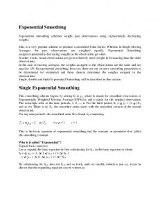
3 Simulations from unstable models In order to demonstrate the problem of instability, we undertook a Monte Carlo study of the AAM model. The instability of the model AAM is linked with the value of the seasonal component. When st−m is close to zero, the values of the level (`t ) and the trend (bt ) components become unstable, as can be seen from the model equations in Table 2. Figure 1 shows 150 observations from one simulated sample path of the AAM model, along with the components of the simulated series, with α = β = γ = 0.2, σ = 1, `0 = 0.1, b0 = 1, s−3 = 0.8, s−2 = 0.6, s−1 = 1.2 and s0 = 1.4. From the top panel of Figure 1, it can be seen that the series is stable until observation 116. It can also be observed that although the series becomes unstable, in this case the seasonal component remains stable. The bottom panel of Figure 1 makes it clear that the cause of the instability is the seasonal component being close to zero at time t = 112.

4 Conclusion In this paper we have shown that eleven of the nonlinear state space models in the exponential smoothing framework are unstable. The unstable models are AMN, AMA, AMd N, AMd A, AMM, AMd M, MMA, MMd A, ANM, AAM and AAd M. Each of these models has undefined forecast mean and infinite forecast variance after the first few forecast horizons. This result holds for any distribution of the error series {ε t } that has positive density at zero. It also holds for any values of the initial state and all non-zero values of the smoothing parameters. The consequence of this result is that these models are of questionable value in forecasting. While it is possible to obtain point forecasts from the models, the point forecasts are not means. Furthermore, forecast intervals derived from variances will be wrong. Consequently, we recommend that only the 19 stable models of the exponential smoothing framework be used.

6

−15 0

50

100

150

0

50

100

150

0

50

100

150

0

50

100

150

0

50

100

150

Sfrag replacements

`t

−400 −150 −4 1.0 2.0 −0.5

st

−8

bt

0

−300

ellt

0

−800

yt

0

−30

yt

0


Figure 1: AAM simulation with α = β = γ = 0.2, σ = 1, `0 = 0.1, b0 = 1, s−3 = 0.8, s−2 = 0.6, s−1 = 1.2 and s0 = 1.4. Top panel: first 116 observations of simulated series. Second panel: all 150 observations of simulated series. Bottom three panels: components of the simulated series.

7


Appendix: Ratio of random variables It is well known that the ratio of two normal random variables, each with mean zero, has a Cauchy distribution and so has undefined mean and infinite variance (see, e.g., Marsaglia 1965). In fact, all even order moments are infinite, and all moments of odd order are undefined. These problems are not apparent in numerical computation if the probability of the denominator being close to zero is very small (for details, see Springer 1979). It is less well-known that the ratio of any two random variables where the denominator has positive density at zero will have the same properties, viz., infinite even order moments and undefined odd order moments. In fact, we could not locate any reference containing this result. So we provide a brief derivation here. Theorem. Let X and Y be two random variables where Y has positive density for all values on an interval including zero. Then the variance and other even order moments of the ratio X/Y are infinite, and the mean and other odd order moments of the ratio X/Y are undefined. Proof. Let f ( x, y) be the joint probability density of ( X, Y ) and note that k

E(| X/Y | ) ≥

Z b Z ε x=a

y=−ε

| x/y|k f ( x, y) dx dy .

for a < b and ε > 0. Choose a, b and ε such that f ( x, y) > C > 0 for x ∈ ( a, b) and y ∈ (−ε, ε). Then, k

E(| X/Y | ) ≥ C

Z b Z ε x=a

y=−ε

µZ k

| x/y| dx dy = C

b x=a

¶ µZ k

| x | dx

ε y=−ε

¶

|y|

−k

dy

by Fubini’s theorem. The second integral is infinite for all k = 1, 2, . . . . The theorem follows.

8


References Aoki, M. & Havenner, A. (1991), ‘State space modelling of multiple time series’, Econometric Reviews 10, 1–59. Hyndman, R. J., Koehler, A. B., Ord, J. K. & Snyder, R. D. (2005), ‘Prediction intervals for exponential smoothing state space models’, Journal of Forecasting 24, 17–37. Hyndman, R. J., Koehler, A. B., Snyder, R. D. & Grose, S. (2002), ‘A state space framework for automatic forecasting using exponential smoothing methods’, International Journal of Forecasting 18(3), 439–454. Marsaglia, G. (1965), ‘Ratio of normal variables and ratios of sums of uniform variables’, Journal of American Statistical Association 60, 193–204. Ord, J. K., Koehler, A. B. & Snyder, R. D. (1997), ‘Estimation and prediction for a class of dynamic nonlinear statistical models’, Journal of American Statistical Association 92, 1621– 1629. Springer, M. D. (1979), The algebra of random variables, Wiley, New York. Taylor, J. W. (2003), ‘Exponential smoothing with a damped multiplicative trend’, International Journal of Forecasting 19, 273–289.

9