SOME OBSERVATIONS ON THE APPLICABILITY OF NORMALIZED COMPRESSION DISTANCE TO STEMMATOLOGY∗ Toni Merivuori1 and Teemu Roos2 1
Department of Computer Science, University of Helsinki, P.O.Box 68, FI-00014 Helsinki, FINLAND,
[email protected] 2 Helsinki Institute for Information Technology HIIT, P.O.Box 68, FI-00014 Helsinki, FINLAND,
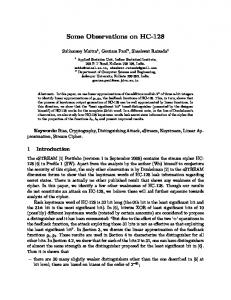
[email protected] ABSTRACT The objective of stemmatology is to construct a familytree of documents that have been generated by a process of repeated duplication and modification. In earlier benchmark experiments on computer-assisted stemmatology, the CompLearn software package was found to perform well on simpler test cases, but it failed to give satisfactory results in a more complex and realistic data set. This was surprising, given the excellent results in related phylogenetic tasks where it was able to reconstruct accurate family-trees of biological species based on their genome sequences. We suggest that the reason for the failure in the complex stemmatological data set is due to difficulties in handling missing data. This explains many features in the incorrect solution produced by CompLearn, and leads to a simple random imputation strategy to fill in the missing values. The strategy is shown to improve the performance by a large margin. 1. INTRODUCTION A prototypical example illustrating the problem studied in stemmatology is as follows: A top AI researcher has finally concluded (after 25 years, see [1]) that the statement “Tweety is a bird” is true. The rumor of this fact spreads around like wildfire, becoming distorted along the way. After a while, a set of scientists submit papers to WITMSE-09 claiming respectively that: “Sweety is a bird,” “Sweety has a bird,” and “Tweety is a nerd.” Can we deduce how the information spread among the scientists? Drawing a graph where each node corresponds to one variant of the message, and each variant is a direct descendant of the message from which it originated, its exemplar, gives us a family-tree of the variants. Such a family-tree, or a stemma, corresponds to i) a clustering hierarchy, where joined subgroups make subtrees; ii) a directed acyclic graph (DAG) of interdocument (causal) dependencies; iii) a network of information flow among the documents; iv) a phylogenetic tree; et cetera. The most widely used tools for inferring such family-trees are based ∗ This work is partially based on an unpublished Master’s thesis “Nor-
malisoitu kompressioet¨aisyys: katsaus sovelluksiin” (in Finnish), Dept. of CS, Univ. Helsinki, by the first author.
Tweety is a bird
Sweety is a bird
Tweety is a nerd
Sweety has a bird
Figure 1. The most likely family-tree of a most unlikely set of statements. (In fact the orientation of the edges, or equivalently the root of the graph, is undetermined by the texts alone.)
on methods developed for phylogenetic analysis, i.e., discovery of evolutionary trees, see [2, 3]. The natural conclusion about Tweety is that “Sweety has a bird” is a result of two distinct, consecutive mutations, the first of which has produced the intermediate form “Sweety is a bird”. Also, it is safe to assume that “Tweety is a nerd” is a result of another, unrelated mutation of the original statement. Hence, we can draw the family-tree shown in Fig. 1. In realistic scenarios, the number of length of the texts is too great to yield to simple manual solution. Furthermore, to make matters infinitely worse, many (often most) of the variants are either completely or partially unknown due to their old age. The core component of the CompLearn package is the normalized compression distance (NCD) [4], defined as NCD(x, y) :=
max{C(x | y), C(y | x)} , max{C(x), C(y)}
(1)
where C(x) is the complexity of string x, and C(x | y) is the conditional complexity of string x given string y. The complexity C(·) is defined using a compression algorithm and can be taken as a computable approximation of Kolmogorov complexity, see [5]. Conditional complexities C(x | y) are evaluated by subtracting the complexity of the conditioning string y from the complexity of the concatenated string xy, i.e., C(x | y) := C(xy) − C(y). The ideal, yet uncomputable, distance metric defined by using Kolmogorov complexity instead of an approxi-
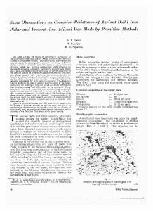
mation thereof has certain universality properties. However, these properties are preserved in the approximation to a degree that depends on the type of objects it is applied to, and the used compressor. In most practical experiments, NCD has given at least satisfactory results, see e.g. [4, 6]. This is remarkable considering that very little or none fine-tuning is required. In this paper, we take a closer look at one application of NCD and CompLearn, namely, stemmatology and in particular, the artificial data set Heinrichi, constructed by copying a text several times by hand for the purpose of evaluating computer-assisted methods [7]. We propose an explanation for the relatively poor performance of CompLearn in this task, and suggest a partial fix by a simple random imputation technique. 2. BENCHMARK DATA SET The main difficulty in evaluating methods for computerassisted stemmatology is the fact that as a rule, we do not have an independent means to determine the correct solution for real-life data sets. The same applies to phylogenetics. In order to enable objective evaluation, artificial manuscript collections have been constructed by copying texts by hand according to a known stemma [7, 8, 9]. Figure 2 shows the correct stemma for the most extensive artificial collection Heinrichi which contains 67 copies of a text, 37 of which are given as input to the methods, while the remaining 30 are hidden in order to make the situation more realistic1 . Furthermore, a variable portion of the words were deleted from some of the 37 input texts so that the lengths of the remaining texts are 1329–8135 characters (symbols). 2.1. Evaluation criterion To measure the closeness of an estimated stemma to the correct one, we use the so called average sign similarity score2 , defined as the percentage of triplets (α, β, γ) of nodes for which the relative order of distances d(α, β) and d(α, γ) differs in the two stemmata. The distance d(α, β) is defined as the number of edges along the shortest path from α to β. In case the inequality d(α, β) > d(α, γ) holds for any three nodes α, β, γ in the estimated stemma if and only if it holds in the correct stemma, then the score is 100 %, otherwise less. In particular, if the estimated stemma is identical to the correct one the score is 100 %. Usually the score is not less than 50 %. For details, see [7]. 2.2. CompLearn’s result Figure 3 shows the result of applying CompLearn to the artificial data set Heinrichi. We use the default gzip compressor in all the presented results; similar outcomes are 1 The data is freely available in several formats (plain text, symbolic, numeric, Nexus) at http://www.cs.helsinki.fi/ teemu.roos/casc/stemma.html. 2 In [7], the score was called average sign distance but since the score measures the similarity, not distance, of the stemmata, we adopt the present terminology.
n
A B C
kA
kB
kAB
Figure 4. Schematic illustration of the pattern of missing text in strings A, B, and C. The length of the substring that is missing in both A and B is kAB . The lengths of the substrings that are missing in either A or B, but not both, are kA and kB , respectively. obtained by other compressors. The average sign similarity score is 53 %, a modest result given that a random guess gives the score of about 50 %, and the best known result is 76 %, see [7]. By looking at the fraction of missing text in each variant (see the bars under each node in Fig. 3), and the location of the variants in the CompLearn stemma, we observe that the variants from which a large portion of text is missing tend to be grouped together even though they are not necessarily closely related in the correct stemma. Although this only explain the errors in the middle branch of the estimated stemma, and there are several other errors in the left-most branch as well, the trend appears to be strong. 3. WHERE AND WHY DOES IT GO WRONG? The tendency of CompLearn to place variants with much missing text together can be explained in terms of the properties of the NCD metric, Eq. (1), by considering the amount of text that is missing in more than one variant at the same position. Roughly, if a sufficient amount of text is missing in two variants, then these two variants will be judged to be more similar to each other than a variant where the text is not missing. This is all quite natural and cannot be taken as a problem as such, but as we will see below, this appears to explain at least some of the problems CompLearn’s result in the Heinrichi data. 3.1. Patterns of missing text Consider three variants, A, B, and C, as depicted in Fig. 4, that are otherwise similar to each other except that a substring of length kA is present in both B and C but missing in string A, and a substring of length kB is missing in B but present in both A and C, and finally, a substring of length kAB is missing in both A and B but present in C. The total length of string C is n. We assume that the strings are labeled so that kB ≤ kA . We make the following two simplifying assumptions:
P
V
O W
Ae
Z
Ba
S
Da
N J
T
I
Cb
Be
Ca
F Bb
Cd Bd
Ad
C
Ac
G
Cc
H
X
Ab
Ce
R B
E
L
K
Cf
M A
Figure 2. The correct stemma of the artificial data set Heinrichi [7]. Labeled nodes denote texts that are given as input to the methods, and the unlabeled internal nodes denote texts that are hidden (not given). Dotted edges denote cases where parts of more than one exemplar have been included in a new copy, a problem known as contamination. Three main branches are colored in green, blue, and red, respectively.
Cb
Bb
H
Bd
X
N
Ca
G
Ad
Z
V
C
Cf
Da
W
Ba
J
Ae
E
A
Cc
Ce
B
K
L
R
T
O
P
M
Be
F
Ab
Ac
Cd
I
S
Figure 3. The stemma obtained by CompLearn for the data set Heinrichi. The tree is manually rooted. Average sign similarity 53% (best score is 76%, see [7]). The bar under each node shows the fraction of observed (non-missing) text in each variant. There is not much resemblance with the correct tree of Fig. 2; the green, blue, and red branches are mixed together. Note that variants from which a large portion is missing (Be, Ca, V, Cf, R, ...) tend to be grouped together in the middle branch.
(A.1) information content is evenly distributed along the strings so that the complexity of any substring is approximately equal to its length, C(x) ≈ l(x), and (A.2) the strings are sufficiently similar in the parts that they share that we can write C(x | y) ≈ 0 for any two substrings at the corresponding positions in two strings. Both approximations are assumed to hold up to o(n) error terms, i.e., terms that are sub-linear in the length of the whole string. Assumption (A.2) implies, for instance, C(A | C) ≈ C(B | C) ≈ 0, and C(B | A) ≈ kA . Proposition 1. Under the above assumptions (A.1) and (A.2), we have
W
0.313
0.497
F
0.595
V
Ca 0.499
W
0.304
F
0.266
0.314
V
Ca 0.321
Figure 5. Left: The CompLearn tree incorrectly connecting F with Ab and C with R, and NCD distances between the four variants. The numbers indicate pair-wise NCD distances. Right: The result of CompLearn after random imputation, see Sec. 4. The tree is now correct.
kA < kAB ≤ n/4 ⇒ NCD(A, B) / NCD(A, C), where the inequality / holds up to o(n) error terms.
3.2. Empirical evidence
Proof. We need to show that kA < kAB ≤ n/4 implies max{C(A | B), C(B | A)} NCD(A, B) = max{C(A), C(B)} max{C(A | C), C(C | A)} < = NCD(A, C). max{C(A), C(C)}
(2)
Under assumptions (A.1) and (A.2), this is approximately equivalent to kA kA kAB < + . (3) n − kB − kAB n n Since the error terms in the numerator and denominator are by assumption (A.2) sub-linear, the equivalence of (2) and (3) holds up to o(n) error terms. The condition kA < kAB ≤ n/4, together with the assumption kB ≤ kA , thus implies n − kB − kAB > n/2 which in turn gives kA kA kA < + . n − kB − kAB n n The required inequality (3) now follows by upper-bounding the second kA on the right-hand side by kAB . The proposition implies that if the part missing in both A and B is larger than the part missing only in A (and as we assumed kB ≤ kA , also the part missing only in B), then A and B are judged to be closer to each other than A is from the whole string C. By essentially the same proof, we get the following similar proposition concerning distances NCD(A, B) and NCD(B, C). Proposition 2. Under assumptions (A.1) and (A.2), we have kA + (kA − kB ) < kAB ≤ n/4 ⇒ N CD(A, B) / N CD(B, C).
(4)
. Furthermore, even if assumption (A.2) is weakened by letting the three strings A, B, C differ from each other by a non-negligible amount, similar results can be obtained by having the gap between kA and kAB sufficiently large (see statement of Propositions 1 & 2).
We note that if we remove words at random, then it is very unlikely that the conditions in Propositions 1 & 2 are realized, and the problem doesn’t usually arise. However, the patterns of missing text in real and artificial manuscripts are not random, and hence, the problem may occur in practice more often than would be expected by chance. We can in fact observe the kind of behavior described above empirically in the Heinrichi data. Let us consider manuscripts Ca, F, V and W, of which the first two belong to the blue (middle) subtree in the correct stemma of Fig. 2, and the latter two belong to the green (left-most) subtree. The patterns of missing text of the Heinrichi data are shown in Figure 6. Each row corresponds to a manuscripts, and white indicates missing text at a particular location. Looking at the patterns of Ca and V it is obvious that both are missing a lot of text, mostly in the beginning. Based on the above theoretical considerations, it is expected that these two variants will be judged to be close to each other in terms of NCD. The left-most stemma in Fig. 5 shows the tree constructed by CompLearn for the four texts. Between the labeled nodes, the figure also shows the NCD distances of neighboring nodes. From the distances we see that V and Ca are incorrectly placed next to each other, and their distance (0.499) smaller than the distance between the two blue variants, Ca and F, and also very close to the distance between the two green variants, V and W. In this case, the short distance between the complete variants, W and F, breaks the tie and results in the incorrect tree. In CompLearn’s result for the whole data, Fig. 3, we also find Ca and V next to each other in the middle branch, together with other incomplete manuscripts. 4. A SIMPLE RANDOM IMPUTATION TECHNIQUE Based on the above considerations about missing text and its effect on NCD, we present a simple random imputation technique to fill in the missing data. In the Heinrichi data, the technique improves the performance of CompLearn by a large margin.
A Ab Ac Ad Ae B Ba Bb Bd Be C Ca Cb Cc Cd Ce Cf Da E F G H I J K L M N O P R S T V W X Z
Figure 6. A graphical display of the Heinrichi data, showing on each row the text of a given variant, indicated by the label on the right, encoded as colors (each word is mapped to a color). White indicates missing words. 4.1. The algorithm The algorithm works by imputing randomly sampled words from the other texts. The texts need to be aligned first so that at each position, the imputed words can be drawn from the same position in the other texts. Algorithm 1 Biased random imputation Input: Set of aligned incomplete strings {A, B, C, . . .}. Output: Set of aligned complete strings. 1: 2: 3: 4: 5: 6: 7: 8:
for all strings s ∈ {A, B, C, . . .} do for all positions i ∈ {1, . . . , n} do while si = empty do si ← sample({Ai , Bi , Ci , . . .}) end while end for end for return {A, B, C, . . .}
In step 4, a missing word si is randomly replaced by a value sampled uniformly from the words {Ai , Bi , Ci , . . .} appearing at the same position in all the texts. This is repeated until a non-empty word is obtained. The algorithm is called biased random imputation since the distribution of the words in the imputation step is the overall distri-
bution at the given position: if a certain word appears in most of the variants, that word is likely to be drawn as a result of sampling uniformly over the variants. In the complete strings thus obtained, the imputed parts are on the average as similar to each other as they are to any other variant. Hence, the pattern of missing words should no longer cause two variants to attract each other in such a great degree. In Fig. 5, the right-most stemma shows how the CompLearn tree and the NCD distances change when the data is imputed: the green and the blue variants are now grouped in the correct way: note in particular that the V–Ca distance, 0.321, is now longer than any of the other distances shown in the figure. 4.2. CompLearn’s result after imputation Figure 7 shows CompLearn’s result for the imputed data. The distinctive difference between the new stemma and the previous one is that now the three main colors are mostly grouped together, even though they cannot be divided completely into three separate branches. For instance, the nodes Be, Ca, and V—all of which were missing a lot of text—are now much better placed (cf. Fig. 2). Also, the group Ad, Z, Ab, G is now correctly placed among the other red variants. Their earlier incorrect placement
R
H
X
Cf
Ac
Be
Ca
V
F
Bb
Bd
T
N
O
Cd
Ae
P
Z
Cc
Ce
Ab
G
M
Cb
C
W
Ad
Da
E
J
A
B
K
L
I
S
Ba
Figure 7. The stemma obtained by CompLearn for the data set Heinrichi after random imputation. The tree is manually rooted. Average sign similarity is now 61%. Notice, for instance, the better placement of variants Be, Ca, and V, as well as Ad, Z, Ab, and G. in the left-most branch cannot be explained so easily, but it may well be caused by the lack of attraction between this group, variant R, and the other red manuscripts due to missing data. The imputed R may now provide sufficient pull to move the quadruple into its more or less correct position. In terms of the average sign similarity, the score improves from 53% to 61%. A similar improvement also occurs with other compressors (bzip2 and blocksort). This still leaves a a gap to the best result, 76%, but nevertheless provides support for our hypothesis about the reason of CompLearn’s previous poor performance in stemmatology. In order to verify these observations, and to minimize the effect of chance, we will run more tests on other complex artificial data sets.
[4]
[5]
[6]
[7]
5. ACKNOWLEDGMENTS This work has been funded in part by the University of Helsinki Research Funds (project STAM).
[8]
6. REFERENCES [1] Robert C. Moore, “Semantical considerations on nonmonotonic logic,” Artificial Intelligence, vol. 25, pp. 75–94, 1985. [2] Peter M. W. Robinson and Robert J. O’Hara, “Report on the Textual Criticism Challenge 1991,” Bryn Mawr Classical Review, vol. 3, no. 4, pp. 331–337, 1992. [3] Matthew Spencer, Klaus Wachtel, and Christoper J. Howe, “The Greek Vorlage of the Syra Harclensis: A comparative stud y on method in exploring textual genealogy,” TC: A
[9]
Journal of Biblical Textual Criticism [http://purl.org/TC ], vol. 7, 2002. Rudi L. Cilibrasi and Paul M. B. Vit´anyi, “Clustering by compression,” IEEE Transactions on Information Theory, vol. 51, no. 4, pp. 1523–1545, 2005. Ming Li and Paul M. B. Vit´anyi, An Introduction to Kolmogorov Complexity and Its Applications, Springer-Verlag, Berlin, 1993. Paul M. B. Vitanyi, Frank J. Balbach, Rudi L. Cilibrasi, and Ming Li, “Normalized information distance,” in Information Theory and Statistical Learning, F. Emmert-Streib and M. Dehmer, Eds., pp. 45–82. Springer-Verlag, New-York NY, 2008. Teemu Roos and Tuomas Heikkil¨a, “Evaluating methods for computer-assisted stemmatology using artificial benchmark data sets,” Literary and Linguistic Computing, 2009, DOI 10.1093/llc/fqp002, Advance Access published on March 14. Matthew Spencer, Elizabeth A. Davidson, Adrian C. Barbrook, and Christopher J. Howe, “Phylogenetics of artificial manuscripts,” Journal of Theoretical Biology, vol. 227, no. 4, pp. 503–511, 2004. Philippe V. Baret, Caroline Mac´e, and Peter Robinson, “Testing methods on an artificially created textual tradition,” in The Evolution of Texts: Confronting Stemmatological and Genetical Methods, Proceedings of the International Workshop held in Louvain-la-Neuve on September 1–2, 2004, C. Mac´e, P. Baret, A. Bozzi, and L. Cignoni, Eds., vol. XXIV–XXV of Linguistica Computazionale. Istituti Editoriali e Poligrafici Internazionali, Pisa-Roma, 2004.