Some remarks and conjectures related to lattice paths in strips along the x-axis Johann Cigler Fakultät für Mathematik, Universität Wien
[email protected]
Abstract In the first part of this paper I give an elementary overview about some number sequences which count various sorts of lattice paths in strips along the x-axis and compute their generating functions in terms of Fibonacci and Lucas polynomials. In the second part I generalize these results by introducing suitable weights and study some special cases in more detail. In the course of this work I have been led to curious number triangles and various conjectures.
0. Introduction Consider lattice paths in 2 of length n which start at the origin (0, 0) and have only upsteps U : (i, j ) (i + 1, j + 1) and down-steps D : (i, j ) (i + 1, j - 1). Equivalently consider (random) walks on which start at 0 , where at each step we go one unit up or down. It is well known that the number of recurrent walks of length 2n is the same as the number of positive walks of length 2n or equivalently that the number of all lattice paths from (0, 0) to (2n, 0) is the same as the number of all non-negative lattice paths of length 2 n. The same holds for the number of all non-negative lattice paths of length 2 n 1 and the number of all lattice paths from (0, 0) to (2n 1, 1). Combining both results let us denote by An the set of all lattice paths of length n which start at the origin and end on height 0 (if n is even) or on height 1 (if n is odd) and let Bn be the
ên ú set of all non-negative lattice paths of length n. Note that each path in An has ê ú up- steps ê2ú ë û ê n + 1ú ú down- steps. Then we have and ê ê 2 ú ë û n An Bn n . 2
(0.1)
The main purpose of this paper is to study paths in An with bounded heights.
Keywords: Lattice paths, Dyck paths, path graph, positive random walks, recurrent random walks, Fibonacci and Lucas polynomials, generating functions, Narayana polynomials, q-analogues, Hankel determinants.
1
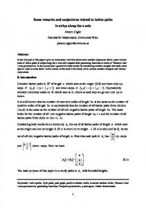
ê k + 1ú ê ú ú £ y £ ê k ú of Let An ,k be the set of all paths in An which are contained in the strip - ê ê 2 ú ê2ú ë û ë û ê k ú ê k + 1ú ú = k. width ê ú + ê ê2ú ê 2 ú ë û ë û For example A5,3 consists of the following 8 paths: DDUDU , DDUUD, DUDDU , DUDUD, DUUDD, UDDDU , UDDUD,UDUDD
Figure 1
Let Bn,k be the set of all paths in Bn which remain in the strip 0 y k . For example B5,3 consists of the following paths: UUUDU , UUUDD, UUDUU , UUDUD, UUDDU , UDUUU ,UDUUD,UDUDU
Figure 2 Then in analogy to (0.1) we have An ,k = Bn ,k
æ ö÷ n çç ÷÷ = å (-1)j ççç ê n + (k + 2)j ú ÷÷. ú÷÷ ç êê j Î ú ÷ø çè ë 2 û
This is essentially known, but we give another proof in the sequel.
2
(0.2)
The set Bn,k can also be interpreted as the set of all walks on the path graph with vertices
0,1,, k . Let M k = (m(0, i, j, k ))
k i , j =1
(
)
= [ i - j = 1]
k i , j =0
be the corresponding adjacency matrix. Note
that m(0, i, j, k ) = 1 if {i, j } is an edge and m(0, i, j, k ) = 0 else, i.e. m(0, 0,1, k ) = 1, m(0, k , k - 1, k ) = 1, and m (i, i 1, k ) = 1 for 0 < i < k . All other entries are 0.
For example 0 1 M3 0 0
1 0 1 0
0 1 0 1
0 0 . 1 0
If we denote by m( n, i, j , k ) the number of non-negative paths from (0, i ) to ( n, j ) in Bn ,k then by the definition of matrix multiplication we get
M kn m(n, i, j , k ) i , j 0 . k
(0.3)
For example 0 5 5 M3 0 3
5 0 8 0
0 8 0 5
3 0 . 5 0
In the first row we see that there are 5 paths from (0, 0) to (5,1) and 3 paths from (0, 0) to (5, 3). k
In the general case we get Bn ,k m( n, 0, j , k ). j 0
A little thought also gives that
k 1 k 1 A2 n ,k m 2n, , ,k 2 2 k 1 k 1 , , k . A2 n 1,k m 2n 1, 2 2 k 1 k to . To see this renumber the rows and columns from 2 2
3
(0.4)
k 1 k 1 , 0 and end in 2n, Then the paths from B2 n,k which start from are mapped 2 2 to the paths from (0, 0) to (2n, 0) in A2 n,k and the paths from B2n1,k which start from k 1 2 , 0 and end in A2 n1,k .
k 1 2n 1, 2 are mapped to the paths from (0, 0) to (2n 1, 1) in
In our example A5,3 m 5, 2,1, 3 8. In the first part of this paper I give an overview about these numbers. Most of these results are known but perhaps my point of view gives a novel approach. In the second part we consider the following weights instead of the numbers An ,k . Define a peak as a vertex preceded by an up-step U and followed by a down-step D , and a valley as a vertex preceded by a down- step D and followed by an up-step U . The height of a vertex is its y - coordinate. The peaks with a height at least 1 and the valleys with height at most - 2 are called extremal points. Thus for example the path UDDUDDU
has two extremal points (1,1), (6, 2) . Let E (v ) be the set of x - coordinates of the extremal points of the path v , e(v ) = E (v ) the number of extremal points of v and i(v ) =
åi
the sum of the x - coordinates of the
i ÎE (v )
extremal points. In [7] and [8] we defined the weight of v by w(v, q ) = q i(v )t e(v ) and considered the polynomials w (An ,k , q ) =
åq
i (v ) e (v )
t
. These polynomials are intimately
v ÎAn ,k
connected with Rogers-Ramanujan type theorems. In the present paper we consider only the case q = 1 and study the polynomials a (n, k , t ) =
åt
e (v )
v ÎAn ,k
in more detail. In our example A5,3 we get a (5,3, t ) t 2 t t 1 t t 2 t t 2 1 4t 3t 2 .
4
(0.5)
The sequences a(n, k , t ) n0 satisfy recurrences of an order k and their generating functions are rational functions of Fibonacci and Lucas polynomials. For n they n n 1 converge to a(n, t ) 2 2 t . Therefore their Hankel determinants 0
d (n, k , t ) det a (i j , k , t ) i , j 0 vanish for n k and converge for each fixed n to n
d ( n, t ) det a (i j , t ) i , j 0 t n
( n 1) 2 4
. Curiously the polynomials d ( n, k , t ) for even k are
multiples of Hankel determinants of a ( n, t ) and for odd k multiples of Hankel determinants N n n 1 j of Narayana polynomials N n (t ) t . j 0 j j 1 n
As far as I know these polynomials have not been considered in the literature. The detailed study of some special cases led to many curious conjectures. Some have been found with the help of the Mathematica package Guess [15] by Manuel Kauers. Of great use has been The On-Line Encyclopedia of Integer Sequences OEIS [19]. If some results are already known please let me know that I can give due credit.
1. Background material
1.1. Lattice paths in strips along the x-axis
Let An ,k be the set of all lattice paths of length n which start at (0, 0) , stop on heights 0 or
ê k + 1ú ê ú ê ú ê ú ú £ y £ ê k ú of width ê k ú + ê k + 1 ú = k . - 1 and are contained in the strip - ê ê 2 ú ê2ú ê ú ê ú ë û ë û ë2û ë 2 û æ n ö÷ çç ÷ ÷ For n £ k all ççç ê n ú ÷÷ paths of length n belong to An ,k . Note that for odd k the strips are not ê ú÷ çç ê ú ÷÷ èë 2 ûø symmetric about the x - axis.
By inclusion – exclusion it has been shown (see e.g. [7],[8] or [9] ) that a(n, k ) := An ,k
æ n ÷÷ö çç ÷ = å (-1) ççç ê n + (k + 2)j ú ÷÷. ê ú÷ çê j Î ú ÷÷ø çè ë 2 û j
(1.1)
We will give a new proof of this result by showing that Bn ,k satisfies (1.1) in Proposition 1.4 and that An ,k Bn , k in Corollary 1.3.
5
The set An ,0 is empty for n > 0 which gives
An ,0
æ n ö÷ çç ÷÷ ÷÷ = éên = 0ùú . = å (-1) ççç ê n ú û ê ú ÷÷ ë j + ç j Î ÷ø çè ëê 2 ûú j
(1.2)
For k = 1 the sets An ,1 consist only of one path. If we denote a path by the sequence of its successive heights this unique path is (0, -1, 0, -1, ). We can write it also as DUDU DUD . Therefore we have
An ,1
æ n ö÷ çç ÷÷ j ç = å (-1) çç ê n + 3 j ú ÷÷ = 1. ú÷÷ ç êê j Î çè ë 2 ûú ÷ø
(1.3)
7 7 7 7 7 For example we have A7,1 1 21 35 21 7 1. 0 2 3 5 6 It is also clear that Bn ,1 consists only of the path UDUDU .
{(0)}, {(0, -1)}, {(0,1, 0), (0, -1, 0)}, {(0,1, 0, -1), (0, -1, 0, -1)}, or {e, {D }, {UD, DU }, {UDD, DUD }, {UDUD,UDDU , DUUD, DUDU }, } if we denote by e
The sets An ,2 are
the trivial path, which gives by induction
An ,2
æ n ö÷ ên ú çç ê ú ÷÷ ê ú j ç = å (-1) çç ê n + 4 j ú ÷÷ = 2 ë 2 û. ú÷÷ çç êê j Î ú÷ 2 èë ûø
(1.4)
There is an easy bijection between An ,2 and Bn,2 . Define D U ,
UD UD, DU UU and UDv UD (v) and DUv UU (v) , where *
( v )
*
exchanges U and D in (v ).
Thus for example UDD UD D UDU , DUD UU D UUD, *
UDUD UDUD, UDDU UD DU UDUU , DUUD UU UD UUDU , DUDU UU DU UUDD. *
*
6
A very interesting case occurs for k = 3. In this case we have An,3 = Fn +1, where Fn is a Fibonacci number.
The Fibonacci numbers Fn =
ê n -1 ú ê ú ê 2 ú ë û
æn - 1 - k ö÷ å çççç k ÷÷÷÷ satisfy Fn = Fn-1 + Fn-2 with initial values k =0 è ø
F0 = 0 and F1 = 1. The first terms are 0,1,1, 2, 3, 5, 8,13, 21, 34, (cf. OEIS [19], A000045). Thus
An ,3
ên ú ê ú æ n ö÷ ê2ú æ çç ë û n - kö ÷ ÷÷ ÷÷ ç j ç ê ú = å (-1) çç n + 5 j ÷ = Fn +1 = å çç ÷. ê ú÷ k ÷÷ø çê ÷ j Î k =0 ç è çè ë 2 ûú ÷ø
Since A0,3 = {0} and A1,3 =
(1.5)
{(0, -1)} we see that the initial values are F
1
= F2 = 1.
Consider now a path in An ,3 . Let the path be given by the sequence of its y - coordinates. If the path ends with (-1, 0) or (0, -1) then the path is the unique continuation of a path in
An-1,3 . If the path ends with (0,1, 0) or (-1, -2, -1) then it is the unique continuation of a path in An-2,3 . Therefore we have
An ,3 = An -1,3 + An-2,3 . This together with the initial
values gives An,3 = Fn +1.
Remark 1.1 æ n ö÷ çç ÷÷ The formula å (-1) ççç ê n + 5 j ú ÷÷ = Fn +1 has been obtained by G.E. Andrews [1], but already ú÷÷ ç êê j Î çè ë 2 úû ø÷ in 1917 I. Schur [25] has studied the right-hand side of the identity j
ên ú ê ú ê2ú ë û
j (5 j -1) én - k ù k ê j ú = 2 q q ( 1) å ê k ú å k =0 j Î êë úûq 2
éæ n öù ÷÷ú êçç êçç ê n + 5 j ú ÷÷ú ÷ú êç ê ÷÷ú êçç ê 2 ú÷ ú û øûúq ëêè ë
én ù én ù for q < 1. Here êê úú = êê úú denotes a q - binomial coefficient defined by êëk úû êëk úûq
( (
) ( ) (
) )
én ù 1 - q ) 1 - q 2 1 - q n -k ê ú =( êk ú (1 - q ) 1 - q 2 1 - q k êë úûq
for 0 £ k £ n and 0 else.
7
(1.6)
It is clear that (1.6) converges to (1.5) for q 1. Therefore (1.6) is called a q - analogue of (1.5). If we let n ¥ in (1.6) we get the famous (first) Rogers-Ramanujan identity
å k ³0
qk
(
2
) (
(1 - q ) 1 - q 2 1 - q k
=
1
) (1 - q ) ¥
j
å (-1)j q
j (5- j ) 2
.
(1.7)
j Î
j =1
For k 3 Thomas Prellberg [22] has found a simple bijection from An ,3 to Bn ,3 : First exchange U and D , remove the last step and append the remaining path to the new first step U . Thus for example we get DDUDU UUDUD UUDU UUUDU or UDDUD DUUDU DUUD UDUUD.
From Figure 1 we get in this way Figure 2. This map is obviously invertible. For a path in Bn ,3 remove the first step U . Then exchange U and D. This gives a path with heights between 2 and 1. Now append the uniquely determined step such that the path ends on height 0 or 1.
Another bijection has been given by Helmut Prodinger [23]. It would be interesting to find simple bijections between An,k and Bn,k for k 3.
Some of the sequences (a(n, k ))
n ³0
occur in the literature in other contexts.
For small values of k useful information can be found in OEIS [19]:
(a(n,2))
is A016116,
(a(n, 3))
is A000045,
(a(n, 4))
= (1,1,2, 3, 6, 9,18,27, ) is A182522,
(a(n, 5))
= (1,1,2, 3, 6,10,19, 33, ) is A028495,
(a(n, 6)) (a(n, 7)) (a(n, 8))
n ³0
= (1,1,2, 3, 6,10,20, 34, 68, ) is A030436,
n ³0
= (1,1,2, 3, 6,10,20, 35, 69, ) is A061551 and
n ³0
= (1,1,2, 3, 6,10,20, 35, 70,125, ) is A178381.
n ³0
n ³0
n ³0
n ³0
8
My interest in these topics has been aroused by the curious formula (1.5) for the Fibonacci numbers. In [6] I tried to put this identity into a general context in order to find an “explanation” of this formula. Among other things I proved that sums of the form (1.1) satisfy some simple recurrences. In the papers [10] – [12] I found simpler proofs and determined the generating functions of these numbers. From [20] I learned the interpretation of these sums as numbers of lattice paths which led to papers [7] – [9]. From this point of view formula (1.5) appears as a special case of the principle of inclusion – exclusion. Later I found in OEIS [19] for the above
mentioned special cases of sequences a ( n, k ) the interpretation as walks in path graphs from which I got new insight into the situation. It turned out that some results which I had previously obtained were already known in other contexts. In the following pages I give an account of my present knowledge of this topic. Remarks and hints to the literature are very welcome.
1.2. Some other combinatorial models Proposition 1.1
The number a (n, 2k + 1) counts all non-negative lattice paths starting from (0, 0) and ending in (n, 0), where besides up-steps and down-steps also horizontal moves (i, 0) (i + 1, 0) on height 0 are allowed and the maximal height of a path is k .
It is easy to find a bijection between these two lattice path models. Starting from the first model we map each up-step (i, -1) (i + 1, 0) and each down-step (i, 0) (i + 1, -1) into a horizontal move (i, 0) (i + 1, 0). The non-negative parts of the path remain unaltered and the negative paths (i, -1) ( j, -1) are reflected on the line y = -
1 into a non-negative 2
path (i, 0) ( j, 0). This map obviously has a unique inverse. For example the set A5,3 is transformed to
Figure 3 In this case the transformation has already been considered in [20].
Corollary 1.1
Consider the graph with vertices 0,1, , k which arises by adjoining a loop at 0 to the path graph with these vertices and let Rk be its adjacency matrix. Then a(n, 2k 1) counts all walks of length n which start and end in 0. Therefore a(n, 2k 1) is the upper-left-most entry in Rkn .
9
Consider for example 2k 1 7. Then we get 1 1 R3 0 0
1 0 1 0
0 1 0 1
0 69 0 55 8 and e.g. R3 48 1 0 20
55 48 20 62 27 28 . 27 42 7 28 7 14
Thus a(8, 7) 69.
Remark 1.2
If we let k ¥ in Proposition 1.1, i.e. consider non-negative lattice paths starting from (0, 0) where besides up-steps and down-steps also horizontal steps (i, 0) (i + 1, 0) on height 0 are allowed then the numbers c(n, j ) of all such paths ending in (n, j ) satisfy
c(n, 0) = c(n - 1, 0) + c(n - 1,1) and c(n, j ) = c(n, j - 1) + c(n, j + 1) for j > 0. We get the following table (cf. OEIS A061554)
(c(n, j ))
n , j ³0
æ1 çç çç 1 1 çç çç 2 1 = çç çç 3 3 çç çç 6 4 çç çè10 10
1 1 4 5
ö÷ ÷÷ ÷÷ ÷÷ ÷÷ ÷÷ ÷÷ 1 ÷÷ 1 1 ÷÷÷ ÷ 5 1 1÷÷ø
(1.8)
. æ n ö÷ æ n ö÷ çç çç ÷ ÷÷ It is easily verified that c(n, j ) = ççç ê n - j ú ÷÷ . Of course we have c(n, 0) = ççç ê n ú ÷÷÷ . ú÷÷ çç êê çç êê ú÷ ÷ è ë 2 úû ÷ø è ë 2 úû ÷ø
If we make the further assumption that c(n, k + 1) = 0 then we get by Proposition 1.1 that c(n, 0) = a(n,2k + 1).
Proposition 1.2
The number a(n,2k ) counts all non-negative lattice paths starting from (0, 0) and ending in (n, n mod 2), where the down-steps (i,1) (i 1, 0) are counted twice and the maximal height of a path is k .
10
Proof
Each path has the form PP 1 2 Pj R where each Pi is either non-negative or non-positive and starts and ends in height 0 and R is empty if n 0 mod 2 and negative if n 1mod 2. We reflect each non-positive Pi on the x axis and let the non-negative ones fixed. Thus each Pi occurs twice. This is accounted for by counting the last down-step twice. The reflected path R ends in (n,1). Thus for k 4 the numbers a (n, 4) n1 1, 2,3, 6,9, count the paths
U , UD , UDU ,UUD , UDUD,UUDD , UDUDU ,UDUUD,UDDU ,UUDUD , , where the bold letters indicate the steps which are counted twice. If we let k and denote by b(n, j ) the weighted number of paths from (0, 0) to (n, j ), n then we get b(n, j ) n 2
j if n j is even and b(n, j ) 0 else. This is OEIS A108044.
Corollary 1.2
Consider the graph with vertices 0,1, , k which arises from the path graph by adjoining a second edge (1, 0) and let Sk be its adjacency matrix. Then a(2n, 2k ) Sk2 n left-most entry in S k2n and a(2n 1, 2k ) S k2 n 1
0,1
0,0
is the upper-
Sk2 n . The last identity is clear 1,1
because each path begins with an up-step.
Consider for example k 3. 0 2 Then S3 0 0
1 0 1 0
0 1 0 1
0 20 0 14 0 0 0 34 0 14 6 and S3 . 28 0 20 0 1 0 0 14 0 6
Thus a(6, 6) 20 and a(7,6) 34.
Proposition 1.3
Let M k = (m(0, i, j, k ))
k i , j =1
(
)
= [ i - j = 1]
k i , j =0
. Then M kn m(n, i, j , k ) i , j 0 , where k
m(n, i, j, k ) denotes the number of paths from (0, i) to (n, j ). If we extend m(n, i, j, k ) by setting
m(n, 0, 2 j , k ) m(n, 0, j , k ), m(n, 0, j k 2, k ) m(n, 0, k 1 j , k ), 11
(1.9)
then we get i
m(n, i, j , k ) m(n, 0, j i 2, k )
(1.10)
0
Proof
We know that m(n 1, i, j , k ) m(n, i, j 1, k ) m(n, i, j 1, k ) for 0 i, j k . Since there are no paths to 1 and to k 1 we also have m(n, i, 1, k ) m(n, i, k 1, k ) 0. There is a uniquely determined extension of m(n, i, j, k ) for j which satisfies m(n, i, j, k ) m(n 1, i, j 1, k ) m(n 1, i, j 1, k ) for all j . This satisfies (1.9). To prove the proposition we show by induction that i
r (n, i, j , k ) m(n, 0, j i 2, k ) equals m(n, i, j , k ). 0
For n 0 we have r (0, i, j , k ) m(0, i, j , k ). If we already know that r (n 1, i, j, k ) m(n 1, i, j, k ) then i
i
0
0
r (n, i, j , k ) m(n, 0, j i 2, k ) m(n 1, 0, j i 2 1, k ) m(n 1, 0, j i 2 1, k ) r (n 1, i, j 1, k ) r (n 1, i, j 1, k ) m(n 1, i, j 1, k ) m(n 1, i, j 1, k ) m(n, i, j , k ).
Thus for k 4 the matrices look like
a(1) a(2) a(3) a(0) a(1) a(3) a(2) a(4) a(1) a(0) a(2) a(2) a(1) a(3) a(0) a(2) a(4) a(1) a(3) a(1) a(3) a(0) a(2) a(3) a(2) a(4) a(4) a(3) a(2) a(1)
a(4) a(3) a(2) a(1) a(0)
Now we can prove that An ,k and Bn ,k have the same size. Corollary 1.3
For all n and k 1 we have An ,k Bn ,k .
12
Proof We know already that
k 1 k 1 A2 n ,k m 2n, , ,k 2 2 k 1 k 1 , , k . A2 n 1,k m 2n 1, 2 2 By (1.10) we get i
m(n, i, j , k ) m(n, 0, j i 2, k ) 0
k 1 k 1 m 2n, , ,k 2 2
k 1 2
k
0
j 0
m(2n, 0, 2, k ) m(2n, 0, j, k ) B
2 n ,k
,
k 1
k k 1 k 1 2 , , (2 1,1, 2 , ) m 2n 1, k m n k m(2n 1, 0, j , k ) B2 n 1,k . 2 2 0 j 0
The next result gives in combination with Corollary 1.3 another proof of (1.1). Proposition 1.4
Bn ,k
n (1) n (k 2) . 2
The following proof uses an idea by S.V. Ault and Ch. Kicey [2]. Proof
We show that for -1 £ j £ k + 1 æ ö÷ æ ö÷ n n çç çç ÷÷ ÷÷ ÷ - å çç ê j + n + 2 ú ÷. m(n, 0, j, k ) = å ççç ê j + n + 1 ú ÷ ÷ ê ú + (k + 2)÷÷ Î çç ê ú + (k + 2)÷÷ Î ç ú ú çè ê ÷ø ÷ø 2 2 èç êë ë û û
(1.11)
To show this formula it suffices to check the recursion and the initial and boundary values. æ ö÷ æ 0 0 ÷÷ö çç çç ÷÷ ÷÷ ÷÷ - å çç ê j + 2 ú m(0, 0, j, k ) = å ççç ê j + 1 ú = [ j = 0]. ç ê ú + (k + 2)÷÷ Î ç ê ú + (k + 2)÷÷÷ Î ç ÷ø ÷ø çè êë 2 úû çè êë 2 úû
Since
13
æ ö÷ æ ö÷ æ ö÷ n n n çç ÷÷ çç ÷÷ çç ÷÷ çç ê n + j + 1 ú ÷÷ = çç ÷÷ = çç ê n - j ú ÷ ê n + j + 1ú çç ê ú + (k + 2)÷÷ ççn - ê ú - (k + 2)÷÷ çç ê ú - (k + 2)÷÷÷ ú ê ú çè ê ÷ø èç 2 2 ø÷ èç ëê 2 ûú ø÷ ë û ë û
we get æ ö÷ æ ö÷ n n çç çç ÷÷ ÷÷ ÷÷ - å çç ê n + 1 ú ÷÷ = 0 m(n, 0, -1, k ) = å ççç ê n ú ç ê ú ÷ ê ú ( 2) ( 2) k j k j + + + + ç ç ÷ ÷÷ j Î ÷ø j Î èç êë 2 úû ÷ø çè êë 2 úû
and
æ ö÷ æ ö÷ n n çç çç ÷÷ ÷÷ ÷÷ - å çç ê k + 2 + n + 1 ú ÷ m(n, 0, k + 1, k ) = å ççç ê k + 2 + n ú ê ú + (k + 2)÷÷ Î çç ê ú + (k + 2)÷÷÷ Î ç ú ú çè ê ÷ø ÷ø 2 2 èç êë ë û û æ ö÷ æ ö÷ n n çç çç ÷÷ ÷÷ ÷÷ - å çç ê k + 2 + n ú ÷÷ = -m(n, 0, k + 1, k ) = å ççç ê k + 2 + n + 1 ú ç ê ú ÷ ê ú ÷÷ + + + + k k ( 2)( 1) ( 2)( 1) ç ç ÷ Î ú ú ÷ø Î çè ê ÷ø çè êë 2 2 û ë û and thus m(n, 0, k + 1, k ) = 0. The recurrence follows from æ n n -1 n -1 ÷÷ö ççæ ÷÷ö ççæ ÷÷ö çç ÷÷ ç ê ÷÷ ç ê ÷÷ çê ú ú ú ççç ê j + n ú + (k + 2)÷÷÷ = ççç ê j - 1 + n - 1 ú + (k + 2)÷÷÷ + ççç ê j + 1 + n - 1 ú + (k + 2)÷÷÷ . ú ú çè ê 2 ú ÷ø çè ê ÷ø çè ê ÷ø 2 2 ë û ë û ë û
Therefore
æ ö÷ æ ö÷ n n çç çç ÷÷ ÷÷ çç ê n ú çç ê n + k + 2 ú ÷ ÷ = m n j k ( , 0, , ) å å ççê ú + (k + 2)÷÷÷ å ççê ú + (k + 2)÷÷÷ j =-1 Î Î ú çè ê 2 ú çè ê ÷ø ÷ø 2 ë û ë û æ n ÷÷ö çç ÷ = å (-1) ççç ê n + (k + 2) ú ÷÷. ê ú÷ çç ê Î ú ÷÷ø 2 èë û k
Remark 1.3
Proposition 1.4 can also be deduced from general results about lattice paths in corridors. E.g. [16], formula (9) implies that the number of walks on Pk +1 from 1 to m is 0 if æ æ n n ÷÷ö ÷÷ö çç çç ÷ ÷÷. n - m º 0 mod 2 and else å çç m + n - 1 ÷÷ - å çç m + n + 1 ç ç + (k + 2)j ÷÷ j Î ç + (k + 2)j ÷÷÷ j Î çè ø è ø 2 2
Both results can be combined to give (1.11). 14
1.3. Some useful facts about the matrices M k
Let us give some more information about the matrices M k . To this end and for later applications we recall some facts about Fibonacci and Lucas polynomials.
The Fibonacci polynomials Fn (x , s ) =
ê n -1 ú ê ú ê 2 ú ë û
æn - 1 - k ö÷ å çççç k ÷÷÷÷x n-1-2ks k satisfy the recurrence relation k =0 è ø
Fn (x , s ) = xFn -1(x , s ) + sFn -2 (x , s ) with initial values F0 (x , s ) = 0 and F1(x , s ) = 1 and the ên ú ê ú ê2ú ë û
æn - k ÷ö n ç ç Lucas polynomials Ln (x , s ) = å ç s k x n -2k satisfy ÷÷÷ k =0 ç è k ÷ø n - k Ln (x , s ) = xLn -1(x , s ) + sLn -2 (x , s ) with initial values L0 (x , s ) = 2 and L1(x , s ) = x .
Most identities about these polynomials can easily be proved by using the well-known Binet formulae
Fn (x , s ) =
an - b n x + x 2 + 4s and Ln (x , s ) = an + b n if a = a(x , s ) = and 2 a-b
x - x 2 + 4s b = b(x , s ) = are the roots of the equation z 2 - xz - s = 0. 2
Let us do this for some formulae which will be needed in the sequel: The identity Ln (x , s ) = Fn +1(x , s ) + sFn -1(x , s )
(1.12)
follows from (an + b n ) (a - b ) = an +1 - b n +1 - ab (an -1 - b n -1 ), the identity F2n (x , s ) = Fn (x , s )Ln (x , s )
(1.13)
from a 2n - b 2n = (an - b n )(an + b n ) and
Fk +1(x, s )2 + sFk (x, s )2 = F2k +1(x, s )
(
from ak +1 - b k +1
)
2
(
- ab ak - b k
)
2
(
)
= (a - b ) a 2k +1 - b 2k +1 .
15
(1.14)
Since a (x + y, -xy ) = x and b (x + y, -xy ) = y we get the well-known identities Ln (x + y, -xy ) = x n + y n , Fn (x + y, -xy ) =
If we choose x = e
jp i k +2
, y =e
-
jp i k +2
x n - yn . x -y
(1.15)
for 1 £ j £ k + 1 we get
æ ö jp Fk +2 ççç2 cos , -1÷÷÷ = 0 or since Fk +2 (x , -1) is a monic polynomial of degree k k +2 è ø÷ k +1 æ j p ö÷ ÷. Fk +2 (x , -1) = ççx - 2 cos ç k + 2 ÷÷ø j =1 è
(1.16)
The Fibonacci polynomials can be represented as the determinant æ x -1 0 0 çç çç-1 x -1 0 çç çç 0 -1 x -1 Fk +2 (x , -1) = det çç çç 0 0 -1 x çç çç çç 0 0 0 çè 0
0ö÷ ÷÷ 0÷÷ ÷÷ 0÷÷ ÷÷ 0÷÷÷ ÷ ÷÷÷ ÷ x ÷÷ø
(1.17)
which follows immediately from their recurrence relation. The right-hand side can be interpreted as the characteristic polynomial of the matrix M k . This is one of the reasons why Fibonacci polynomials play such a dominant role in this field. I became aware of this fact through the blog post [27] by Qiaochu Yuan.
By (1.16) the eigenvalues of M k are given by lj = 2 cos
jp for 1 £ j £ k + 1. k +2
Then v j = (F1(lj , -1), F2 (lj , -1), , Fk +1(lj , -1)) is an eigenvector corresponding to lj . t
For M k v j = lj v j is equivalent with F-1 (lj , -1) + F +1 (lj , -1) = lj F (lj , -1) for 1 £ £ k + 1.
Note that F0 (lj , -1) = Fk +2 (lj , -1) = 0. j p j pi j pi sin jp e k +2 - e k +2 k +2 Since by (1.15) F (lj , -1) = F (2 cos , -1) = j pi = j pi k +2 jp sin e k +2 - e k +2 k +2
16
t
æ jp 2j p (k + 1)j p ö÷ ÷. , sin , ,, sin the eigenvectors are (up to scaling) given by v j = çççsin k +2 k + 2 ÷÷ø è k +2 2 v since k +2 j
The normalized eigenvectors are
2 2 j p ö k +1 æ 2 j p i æ ö ççe k +2 - 2 + e - k +2 i ÷÷ = - 1 -4 - 2k = k + 2 . ççsin j p ÷÷ = - 1 ( ) 2 ÷÷ å çè k + 2 ÷÷ø å 4 =1 ççè 4 =1 ø÷ k +1
Since M k is obviously symmetric we see that the matrix
æ ö÷ 2 2 2 ç U = çç v1, v2 , , vk +1 ÷÷÷ ççè k + 2 k +2 k +2 ø÷ is orthogonal. Let Lk = (lj [i = j ])
k +1 i , j =1
be the diagonal matrix whose entries are the
eigenvalues. Then M k = U LkU -1 = U LkU t . Therefore from M kn = U LnkU t we get the known trigonometric representation n
2 k +1 p j p æç j p ÷ö m(n, 0, j, k ) = sin sin 2 cos ç å k + 2 k + 2 çè k + 2 ÷÷÷ø . k + 2 =1
(1.18)
References may be found in the recent paper [14] by Stefan Felsner and Daniel Heldt where similar results are obtained and in the survey article [17] by Christian Krattenthaler.
1.4. Generating functions
The generating functions of these number sequences turn out to be quotients of Fibonacci and Lucas polynomials or equivalently quotients of Chebyshev polynomials. In the same way as above we see that det (I k - M k x ) = Fk +2 (1, -x 2 ). -1
From (I k - M k x )
-1
= å M kn x n and Cramer’s Rule (I k - M k x ) n ³0
=
adj (I k - M k x )
det (I k - M k x )
we find by considering the top-left entry of these matrices that the generating function vk ( x) of the numbers m(n, 0, 0, k ) is given by
vk ( x) m(n, 0, 0, k ) x m(2n, 0, 0, k ) x n
n0
n
n0
17
Fk 1 1, x 2
Fk 2 1, x 2
.
(1.19)
Helmut Prodinger has kindly brought my attention to the paper [3] by N.G. de Bruijn, D.E. Knuth and S.O. Rice which gives another approach to this formula. The numbers m(2n, 0, 0, k ) count the Dyck paths with height k . Such a path P is either the trivial path (0, 0) (0, 0) of length 0 or has a uniquely determined decomposition P = UP1DUP2D UPj D where each Pi is a Dyck path with height £ k - 1. Therefore vk ( x) satisfies
(
) (
)
2
3
vk (x ) = 1 + x 2vk -1(x ) + x 2vk -1(x ) + x 2vk -1(x ) + =
1 . 1 - x 2vk -1(x )
(1.20)
Note that v 0 (x ) = 1. For arbitrary Dyck paths (1.20) gives the well-known fact that v(x ) = v¥ (x ) =
1 æç2n ö÷÷ 1 1 - 1 - 4x 2 2n ç ÷ or where C = v ( x ) = = C x å n n n + 1 ççè n ÷÷ø 2x 2 1 - x 2v(x ) n ³0
is a Catalan number. This implies that m(2n, 0, 0, k ) = C n for n £ k . From (1.20) we deduce the well-known generating function of bounded Dyck paths
vk (x ) =
Fk +1(1, -x 2 ) Fk +2 (1, -x 2 )
.
(1.21)
For this holds for k = 0. If it is true for k - 1 then 1 1 vk (x ) = = 2 2 x Fk (1, -x 2 ) 1 - x vk -1(x ) 1Fk +1(1, -x 2 ) Fk +1(1, -x 2 ) Fk +1(1, -x 2 ) = = . Fk +1(1, -x 2 ) - x 2Fk (1, -x 2 ) Fk +2 (1, -x 2 ) Let now more generally
vk (x, j ) = å m(n, 0, j, k )x n .
(1.22)
n ³0
Since each path P from (0, 0) to (n, j ) has a unique decomposition
P = PUPUP UPj where P is a Dyck path bounded by k we get 0 1 2 vk (x , j ) = x j vk (x )vk -1 (x ) vk - j (x ).
18
(1.23)
By (1.23) and (1.21) we get
vk ( x, j ) x
j
Fk j 1 1, x 2 Fk 2 1, x 2
.
(1.24)
As shown in [6] and [10] the generating functions of the sequences (a (n, k ))
n ³0
å a(n,2k + 1)x n = n ³0
Fk +1(1, -x 2 )
are given by
(1.25)
Fk +2 (1, -x 2 ) - xFk +1(1, -x 2 )
and
å a(n,2k )x
n
=
Fk +1(1, -x 2 ) + xFk (1, -x 2 ) Lk +1(1, -x 2 )
n ³0
.
(1.26)
ê k + 1ú ú. Observe that deg (Fk +2 (1, -x 2 ) - xFk +1(1, -x 2 )) = k + 1 and deg Lk +1(1, -x 2 ) = 2 ê ê 2 ú ë û
Since by (1.14) and (1.13) Fk +1(1, -x 2 ) 2
2
Fk +2 (1, -x ) - xFk +1(1, -x )
=
(
)
Fk +1(1, -x 2 ) Fk +2 (1, -x 2 ) + xFk +1(1, -x 2 ) 2
F2k +3 (1, -x )
and Fk +1(1, -x 2 ) + xFk (1, -x 2 ) Lk +1(1, -x 2 )
=
(
)
Fk +1(1, -x 2 ) Fk +1(1, -x 2 ) + xFk (1, -x 2 )
(
F2k +2 1, -x 2
)
both formulae (1.25) and (1.26) can be written compactly as F k 2 1, x 2 F k 3 1, x 2 xF k 1 1, x 2 2 2 2 . n a ( n, k ) x 2 Fk 2 1, x n0
(1.27)
Let us give another proof of these formulae. -1
As above (I k - Rk x )
-1
= å Rkn x n and Cramer’s Rule gives (I k - Rk x ) n ³0
19
=
adj (I k - Rk x )
det (I k - Rk x )
.
1 x x 0 1 x x 0 x 1 det I k xRk det 0 0 0 0 0 0
0 0 0 0 2 2 Fk 2 1, x xFk 1 1, x . 1 x x 1
0 0
For by expanding with respect to the first column we get (1 x ) Fk 1 1, x 2 x 2 Fk 1, x 2 Fk 2 1, x 2 xFk 1 1, x 2 . Thus we get again
å a(n,2k + 1)x
n
n ³0
=
(
Fk +1 1, -x 2
(
)
) (
Fk +2 1, -x 2 - xFk +1 1, -x 2
)
.
Let 1, x 2 and 1, x 2 . Then the right-hand side can also be written as
k 1 k 1 . k 2 k 2 x k 1 k 1 -1
By Corollary 1.2 we get (I k - Sk x ) 1 x 0 2 x 1 x 0 x 1 det I k Sk x det 0 0 0 0 0 0
-1
= å Skn x n and (I k - Sk x ) n ³0
=
adj (I k - Sk x )
det (I k - Sk x )
.
0 0 0 0 2 Lk 1 1, x , 1 x x 1 0 0
because Fk 1 1, x 2 2 x 2 Fk 1, x 2 Fk 2 1, x 2 x 2 Fk 1, x 2 Lk 1 1, x 2 . By considering the upper-left-most entry we get
a(2n, 2k ) x n0
2n
Fk 1 1, x 2 Lk 1 1, x 2
1 k 1 k 1 . k 1 k 1
For k this converges to the well-known formula
2n
n x n0
20
n
1 1 . 1 4 x2
By considering the entry (1,1) we get in the same way
a(2n 1, 2k ) x
2n
n 0
Fk 1, x 2
Lk 1 1, x 2
.
Thus (1.26) is proved. Another derivation of (1.27) is due to Helmut Prodinger (personal communication): k
Since ak (x ) = å vk (x , j ) we have to show that j =0
F k 2 1, x 2 F k 3 1, x 2 xF k 1 1, x 2 2 k 2 2 2 x j Fk j 1 1, x . Fk 2 1, x 2 Fk 2 1, x 2 j 0
This is equivalent with Fk21 1, x 2 x 2 j F2 k 2 j 1 1, x 2 , j
Fk 1 1, x 2 Fk 1, x 2 x 2 j F2 k 2 j 1, x 2 . j
The first identity reduces to k 2 k 2 j 1 2 k 2 j 1 1 2 k 1 k 2 k 1 ( ) j 0 j 0 j 0 j
k
j
2 k 1 k 1 k 2 k 1 k 1 k k 1 k 1 2 ( ) 2
j
and the second one to k 2k 2 j 2k 2 j 1 2k k 2k ( ) j 0 j 0 j 0 j
k
j
j
2 k k 1 k 1 2 k k 1 k 1 k 1 k 1 k k . ( ) 2
21
(1.28)
2. Polynomials associated with An,k . 2.1. Definitions and known results
Instead of the numbers An ,k we consider the following weights. Define a peak as a vertex preceded by an up-step U and followed by a down-step D , and a valley as a vertex preceded by a down- step D and followed by an up-step U . The height of a vertex is its y coordinate. The peaks with a height at least 1 and the valleys with height at most -2 are called extremal points. Let E (v ) be the set of x - coordinates of the extremal points of the path v , e(v ) = E (v ) the number of extremal points of v and i(v ) =
åi
the sum of the
i ÎE (v )
x - coordinates of the extremal points.
Following [20] we defined in [7] and [8] the weight of v by w(v, q ) = q i(v )t e (v ) and considered the polynomials w (An ,k , q ) =
åq
i (v ) e (v )
t
. These polynomials are intimately connected with
v ÎAn ,k
Rogers-Ramanujan type theorems. In the present paper we consider only the case q = 1 and study the polynomials a(n, k, t ) =
åt
e (v )
(2.1)
v ÎAn ,k
ên ú in more detail. It is obvious that deg (a(n, k, t )) = ê ú for k > 1 because the maximal ê2ú ë û degree is obtained by the path UDUD .
æn ö÷ ç If we set çç ÷÷ = 0 for n < 0 it follows from the results in [7] and [8] that for k ³ 1 these çèk ÷÷ø polynomials can be written in the following form: æ öæ ö çç êê n + (k - 2)j úú ÷÷ çç êê n + 1 - (k - 2)j úú ÷÷ ú ÷÷÷ çç ê ú ÷÷÷t a(n, k, t ) = å (-1)j å ççç êë 2 2 û÷çë û÷ ÷ çç ÷ j Î ³ j ç çè -j +j ÷øè ø÷
(2.2)
For t = 1 we have of course a(n, k,1) = An ,k . Remark 2.1
A direct proof that (2.2) implies æ ö÷ n çç ÷÷ a(n, k,1) = å (-1)j ççç ê n + (k + 2)j ú ÷÷ ú÷÷ çç êê j Î ú ÷ø 2 èë û
22
(2.3)
ê n + kj ú ê n + 1 - kj ú ú+ê ú = n. follows from the fact that ê ê 2 ú ê ú 2 ë û ë û
For æ ê n + (k - 2)j ú ÷ö÷ æ ê n + (k - 2)j ú öæ æ ê n + (k - 2)j ú ö÷ çç ê n + 1 - (k - 2)j ú ö÷ ê ú n ÷ ÷÷ ç ç ç ¥ ê ¥ ê ú ÷÷ ç ê ú ÷÷ ú ÷÷ çç ê ú çç çç 2 ÷÷ ç ë û ê ú ê ú ê ú ç ÷ ÷ ÷ 2 2 2 å çççë ÷ û ÷÷ çç ë û ÷÷ = å çç ë û ÷ç ê ú ÷ ÷ çç ÷ = j çç ÷÷ ççn - ê n + (k - 2)j ú - - j ÷÷÷ = j ç + j j j ÷ ÷ ÷ç è øè ø è ø çç ÷ ê ú 2 è ø÷ ë û æ ö÷ ê n + (k - 2)j ú æ ê n + (k - 2)j ú ÷ö çç ê ú n ÷÷÷ ¥ çê ú÷÷ çç ê ú çç 2 ÷÷ ë û ê ú ÷ç = å çç ë 2 ÷÷ û ÷ç ê ú ÷ ç n ( k 2) j + ÷ çn - ê i =-¥ ç ú - i - 2 j ÷÷ çè ÷ø÷ç i ê ú ÷ø÷ çèç 2 ë û
æ ê ú ö æ ê n + (k - 2)j ú ö÷ çç n - ê n + (k - 2)j ú ÷÷ æ ö÷ æ ö÷ n n ç ¥ çê ú÷÷ çç ÷÷ çç ÷ ê ú ÷÷÷ çç 2 ë û ÷ = çç ê n + 1 - (k + 2)j ú ÷÷ = çç ê n + (k + 2)j ú ÷÷÷ . ú ÷÷ çç = å ççç ëê 2 û ÷ ç ê n + 1 - (k + 2)j ú ú÷÷ çç ê ú÷÷ ÷÷ ç ê ÷ç ê i =-¥ ç ú - i ÷÷ çèç ê ú ø÷ èç ê ú ø÷ i ÷ø çç ê çè 2 2 ÷ ë û ë û ú ÷ çè ë 2 ø û æ öæ ö çç êê n úú ÷÷ çç êê n + 1 úú ÷÷ ÷ ÷ For n £ k we have a(n, k, t ) = å ççç êë 2 úû ÷÷ ççç êë 2 úû ÷÷t . ÷÷ ç ÷÷ ³0 ç çè ÷øèç ÷ø
The simplest special cases are a(n,1, t ) = 1, ên ú ê ú ê2ú ë û
a(n,2, t ) = (1 + t ) .
As a generalization of (1.5) we get ên ú ê ú ê2ú ë û
æ öæ ö çç êê n + j úú ÷÷ çç êê n + 1 - j úú ÷÷ æn - k ö÷ ÷ ÷ çç ÷÷t k = å (-1)j å çç ê 2 ú ÷÷ çç ê ú ÷÷t . a(n, 3, t ) = Fn +1(1, t ) = å ç 2 ë û ÷ç ë û÷ ç ÷ k ÷ ç ÷ç ÷ k =0 è j Î ³ j ç ø çè - j ÷øèç + j ÷ø
(2.4)
The first terms of a(n, 3, t ) are
(1,1,1 + t,1 + 2t,1 + 3t + t ,1 + 4t + 3t ,1 + 5t + 6t 2
2
2
)
+ t 3 ,1 + 6t + 10t 2 + 4t 3 ,
To show that a(n, 3, t ) = Fn +1(1, t ) consider a path in An,1. If the next to the last point is not extremal then the path is the unique continuation of a path in An-1,1, if it is extremal then the last two steps are a peak or a valley and the rest of the path belongs to An -2,1. Therefore we have a(n,1, t ) = a(n - 1,1, t ) + ta(n - 2,1, t ). The initial values are a(0,1, t ) = a(1,1, t ) = 1.
23
2.2. Generating functions for the polynomials a(n, k, t ). 2.2.1.
We now want to determine the generating functions for the polynomials a(n, k, t ). To this end we introduce the polynomials n ( x, t ) Fn 1 (1 t ) x 2 , x 2 x 2 Fn 1 1 (1 t ) x 2 , x 2 .
(2.5)
They satisfy n ( x, t ) 1 (1 t ) x 2 n 1 ( x, t ) x 2 n 2 ( x, t ) with initial values 0 ( x, t ) 1 ( x, t ) 1. For t 1 we get n ( x,1) Fn 1 1, x 2 .
Theorem 2.1
For k ³ 0 the generating function of the sequence a (n, 2k 1, t ) n0 is
å a(n,2k + 1, t )x n ³0
n
=
Fk (x , t ) Fk +1(x , t ) - x Fk (x , t )
.
(2.6)
For the proof we first observe that for the polynomials a(n, 2k 1, t ) Proposition 1.1 remains true if we define the weight of a non-negative lattice path p by w( p ) t e ( p ) where e( p) denotes the number of peaks of p. Proposition 2.1
The polynomial a(n,2k + 1, t ) is the weight of all non-negative lattice paths starting from (0, 0) and ending in (n, 0), where besides up-steps and down-steps also horizontal moves (i, 0) (i + 1, 0) on height 0 are allowed and the maximal height of a path is k . Proof of Theorem 2.1
Let A(k , x, t ) be the generating function of these lattice paths and let D(k , x, t ) be the generating function of all Dyck paths with maximal height k with the same weight. Then A(k , x, t ) 1 xA(k , x, t ) x 2tA(k , x, t ) x 2 D(k 1, x, t ) 1 A(k , x, t )
because such a path is either trivial or begins with a horizontal step or with UD or with UPD where P is a non-trivial Dyckpath of height k 1. Therefore we get A(k , x, t )
1 . 1 x x t x x 2 D (k 1, x, t ) 2
2
24
Since D(0, x, t ) 1 we get A(1, x, t )
1 . 1 x x 2t
In order to compute A(k , x, t ) we must first compute D(k , x, t ). Here we have D (k , x, t ) 1 x 2tD(k , x, t ) x 2 D(k 1, x, t ) 1 and thus D ( k , x, t )
1 . 1 x t x x 2 D (k 1, x, t )
(2.7)
k ( x, t ) . k 1 ( x, t )
(2.8)
2
2
This gives D ( k , x, t ) This follows by induction because 1 1 (1 t ) x 2 x 2
k 1 ( x, t ) k ( x, t )
k ( x, t ) ( x, t ) k . 2 1 (1 t ) x k ( x, t ) x k 1 ( x, t ) k 1 ( x, t ) 2
Then we get 1
A(k , x, t )
1 (1 t ) x 2 x x 2
k 1 ( x, t ) k ( x, t )
k ( x, t ) . k 1 ( x, t ) x k ( x, t )
If we let k in (2.7) we get the generating function D( x, t ) of all Dyck paths with weight given by the number of peaks w( p ) t e ( p ) (cf. [13]) D ( x, t )
1 (1 t ) x 2
1 (1 t ) x
2 2
2x
2
4 x2
N n (t ) x 2 n .
(2.9)
n0
1 n n n k t for n 0 and N 0 (t ) 1 denotes a Narayana polynomial (cf. n k 0 k k 1 OEIS A001263 or [18]). Note that there is a certain ambiguity of notation in the literature. In N (t ) Petersen [21] the polynomials Cn (t ) n for n 0 with C0 (t ) 1 are called Narayana t polynomials. In [18] these polynomials are called associated Narayana polynomials. Here N n (t )
25
If we let k in A(k , x, t ) we get the generating function
æ æ ê n ú öæ ê n + 1 ú ö ö÷ çç çç ê ú ÷÷çç ê ÷ ÷ 1 çç çç ê 2 ú ÷÷çç ê 2 úú ÷÷÷t ÷÷x n = . å ççå ççë û ÷÷÷ççë û ÷÷ ÷÷÷ 2 2 1 (1 ) ( , ) + t x x x D x t ÷ n ³0 ç ³0 ÷ èç çè ÷øèç ÷ø ø÷
(2.10)
In an analogous manner we introduce the polynomials
Ln (x , t ) = Ln (1 + (1 - t )x 2 , -x 2 ) - x 2Ln -1(1 + (1 - t )x 2, -x 2 ).
(2.11)
They satisfy n ( x, t ) 1 (1 t ) x 2 n 1 ( x, t ) x 2 n 2 ( x, t ) with initial values
0 ( x, t ) 1 (1 t ) x 2 and 1 ( x, t ) 1 (1 t ) x 2 . For t 1 we get n ( x,1) Ln 1 1, x 2 .
Theorem 2.2
For k ³ 1 the generating function of a (n, 2k , t ) n0 is
å a(n,2k, t )x
n
=
Fk (x , t ) + x Fk -1(x , t ) Lk (x , t )
n ³0
.
(2.12)
Proof
Let B(k , x, t ) a(2n, 2k , t ) x 2 n . n0
Then B (k , x, t ) 1 x 2tB (k , x, t ) x 2 B (k , x, t ) 2 x 2 D(k 1, x, t ) 1 B (k , x, t ) because each path is either empty or begins with UD or with DU or has the form UPD or DPU where P is a Dyck path with height k 1 and P a reflected Dyck path with height k 1 . Therefore B ( k , x, t )
1 1 2 1 x t x 2 x D (k 1, x, t ) 1 (1 t ) x 2 2 x 2 k 1 ( x, t ) k ( x, t ) 2
2
k ( x, t ) ( x, t ) . k 2 k 1 ( x, t ) x k 1 ( x, t ) k ( x, t )
26
Let C (k , x, t ) a(2n 1, 2k , t ) x 2 n 1. n
Then C (k , x, t ) xD(k 1, x, t ) B(k , x, t ) because each path ends with DP where P is a reflected path of P D(k 1, x, t ). Therefore we get ( x, t ) k ( x, t ) ( x, t ) C (k , x, t ) x k 1 x k 1 k ( x, t ) k ( x, t ) k ( x, t ) If we let k in the formula F (x , t ) 1 å a(2n,2k, t )x 2n = Lk (x, t ) = 1 - x 2t + x 2 - 2x 2D(k - 1, x, t ) and observe (2.9) we get n ³0 k n n 2 k 2 n t x n0 k 0 k
1
1 (1 t ) x 2 4 x 2 2
.
(2.13)
2.2.2.
Let us now consider some special cases. The simplest special cases are ên ú
ê ú ê2ú n 1+x 1+x ë û a ( n ,2, t ) x = = = (1 + t ) x å å 2 2 2 (1 + (1 - t )x ) - 2x 1 - (1 + t )x n ³0 n ³0 n
and
å a(n, 3, t )x
n
n ³0
=
1 1 = = å Fn +1(1, t )x n . 2 2 (1 + (1 - t )x ) - x (x + 1) 1 - x - tx n ³0
Let us also consider a(n, 4, t ). The first terms are 1,1,1 + t,1 + 2t,1 + 4t + t 2 ,1 + 5t + 3t 2,1 + 7t + 9t 2 + t 3 ,1 + 8t + 14t 2 + 4t 3, . Here we have 1 + x - tx 2
å a(n, 4, t )x = 1 - x - 2tx - tx + t x = å a(2n, 4, t )x + x å a(2n + 1, 4, t )x . n
2
n ³0
2n
n ³0
2
4
2
4
=
1 - tx 2 1 +x 2 2 4 2 4 2 2 1 - x - 2tx - tx + t x 1 - x - 2tx - tx 4 + t 2x 4
2n
n ³0
1 - tx 2 x 2 + tx 2 (1 - tx 2 ) + tx 4 -1 = Since 1 - x 2 - 2tx 2 - tx 4 + t 2x 4 1 - x 2 - 2tx 2 - tx 4 + t 2x 4 we get by comparing coefficients and setting a(-1, 4, t ) = 0
27
a(2n + 3, 4, t ) = a(2n + 2, 4, t ) + ta(2n + 1, 4, t ) a(2n + 2, 4, t ) = a(2n + 1, 4, t ) + ta(2n, 4, t ) + ta(2n - 1, 4, t ) Thus the polynomials a(n, 4, t ) can easily be computed. 2n
Let now b(n, t ) = a(2n, 4, t ) + ta(2n - 1, 4, t ) = å bn ,k t k . Then the table (bn ,k ) begins as 2
2
k =0
follows æ ö÷ 1 çç ÷÷ çç ÷÷ 1 1 1 çç ÷÷ çç ÷÷ 1 1 4 2 1 ÷÷ çç ÷÷ çç 1 1 7 5 9 3 1 ÷÷ çç çç 1 1 10 8 26 14 16 4 1 ÷÷÷ ÷ çç çè1 1 13 11 52 34 70 30 25 5 1ø÷÷
(2.14)
The sum of the rows is b(n,1) = a(2n, 4,1) + a(2n - 1, 4,1) = 2 ⋅ 3n -1 + 3n -1 = 3n and the alternating sum is 2n
å (-1) b k =0
k
n ,k
= a(2n, 4,1) - a(2n - 1, 4,1) = 2 ⋅ 3n -1 - 3n -1 = 3n -1.
The table (bn ,k ) satisfies
bn,2k +1 = bn-1,2k -1 + bn -1,2k , bn,2k = bn -1,2k -2 + 2bn -1,2k -1 + bn -1,2k .
(2.15)
n n n 2n k n 2n k 1 b It seems that b2 n,2 n and 2 n 1,2 n 1 . k k k 0 k k 0 k
2.3. Generating functions of the coefficients Theorem 2.3
For each k 0 there exist polynomials u j ( x, 2k 1) with integer coefficients such that x 2u1(x ,2k + 1) x 4u2 (x ,2k + 1) 2 x 6u 3 (x ,2k + 1) 3 1 å a(n,2k + 1, t )x = 1 - x + (1 - x )2 t + (1 - x )3 t + (1 - x )4 t + . n ³0 (2.16) n
k
Especially we have u1 ( x, 2k 1) x 2 j 2 and u j (1, 2k 1) k j . j 1
28
Proof
By induction it is easily verified that n ( x, t ) 1 tx 2 c1 x 2 t 2 x 4 c2 x 2 with c1 x 2 (n j ) x 2 j 2 and n
j 1
deg c j ( x 2 ) 2n 2.
Therefore Fk +1(x , t ) - x Fk (x , t ) = 1 - x + tx 2 p1(x ) + t 2x 4 p2 (x ) + + t k x 2k pk (x ) for some polynomials p j ( x) with deg p j 2k . By multiplying both sides of (2.16) with Fk +1(x , t ) - x Fk (x , t ) we get
(F (x, t ) - x F (x, t )) å a(n,2k + 1, t )x = (1 - x + tx p (x ) + t x p (x ) + + t x p (x )) n
k +1
k
n ³0
2
2
k
4
1
2k
k
2
2 4 6 æ 1 ö÷ x u1 (x , 2k + 1) x u 2 (x , 2k + 1) 2 x u 3 (x , 2k + 1) 3 ç ÷÷ = Fk (x , t ). + t + t + t + * çç 2 3 4 (1 - x ) (1 - x ) (1 - x ) èç 1 - x ø÷
Since the highest power of t in Fk (x , t ) is t k 1 we see that the coefficient of t n vanishes for
n k. Comparing coefficients of t n we get un ( x, 2k 1) un 1 ( x, 2k 1) u ( x, 2k 1) p1 ( x) n k pk ( x) cn x 2 n n n 1 k (1 x) (1 x) (1 x)
where cn x 2 0 for n k . This is equivalent with un ( x, k ) p1 ( x)un 1 ( x, 2k 1) (1 x) p2 ( x)un 2 ( x, 2k 1) cn x 2 (1 x) n (2.17) Therefore un ( x, k ) is a polynomial with integer coefficients. Let us compute u1 ( x, 2k 1) p1 ( x) (1 x)c1 x 2 . n
n
j 1
j 1
We get p1 ( x) (k j ) x 2 j 2 x (k 1 j ) x 2 j 2 . This implies
u1 ( x, 2k 1) p1 ( x) (1 x)c1 x 2 (k 1 j ) x 2 j 2 x (k j ) x 2 j 2 (1 x) (k j ) x 2 j 2 k
k
k
j 1
j 1
j 1
k
k
k
j 1
j 1
j 1
(k 1 j ) x 2 j 2 (k j ) x 2 j 2 x 2 j 2 .
29
Thus u1 (1, 2k 1) k and by (2.17) we get u j (1, 2k 1) k j . Some special cases.
For k 0 we get u j ( x, 0) 0. For k 1 we have F2 (x , t ) - x F1(x , t ) = 1 - x - tx 2 and therefore p1 ( x ) 1. This implies un ( x,1) 1 for all n. Thus we get
å a(n, 3, t )x n = n ³0
1 x 2j j = t å (1 - x )j +1 . 1 - x - tx 2 j ³0
Let us also consider k 2. Here we get F2 (x , t ) = 1 - tx 2 and
(
)
F3 (x , t ) - x F2 (x , t ) = 1 - x + tx 2 -2 + x - x 2 + t 2x 4 This implies u1 ( x,5) 2 x x 2 (1 x) 1 x 2 and
u j (x , 5) = (2 - x + x 2 )u j -1(x , 5) - (1 - x )u j -2 (x , 5)
(2.18)
for j 2. Theorem 2.4
For k 1
å a(n,2k, t )x n = n ³0
x 2v1(x ,2k ) x 4v2 (x ,2k ) x 6v 3 (x ,2k ) 1 2 + + + t t t3 + 2 3 2 4 3 1 - x (1 - x ) (1 + x ) (1 - x ) (1 + x ) (1 - x ) (1 + x )
for some polynomials v j ( x, 2k ) with integer coefficients. Moreover v1 ( x, 2k )
2 k 2
x
j
and
j 0
v j (1, 2k ) (2k 1) j ,
(2.19)
v j (1, 2k ) (2k 1) j 1. Proof
( )
( )
By multiplying both sides with Lk (x , t ) = 1 - x 2 + tx 2h1 x 2 + + t k x 2k hk x 2 we get Lk (x , t )å a(n,2k, t )x n n ³0
(
= 1 - x + tx h 2
2
(x ) + + t x 2
k ,1
k
2k
æ
( ))çççç
hk ,k x
2
1
è1 - x
x v 1 (x , 2k ) 2
+
2
(1 - x ) (1 + x )
= Fk (x , t ) + x Fk -1(x , t ).
30
x v 2 (x , 2k ) 4
t +
3
x v 3 (x , 2k ) 6
2
2
(1 - x ) (1 + x )
t +
4
(1 - x ) (1 + x )
3
3
ö÷ ÷ø
t + ÷ ÷
As above we see that each v j ( x, 2k ) is a polynomial with integer coefficients and that v1 ( x, 2k )
2k 2
x . Since deg h j
k, j
j 0
2k 2 j it follows that deg v j (2k 2) j.
By induction we see that hk ,1 x 2 k x 2 x 4 x 2 k 2 . Therefore we get that the leading coefficient of v j ( x, 2k ) is 1 and that v j (1, 2k ) hk ,1 (1)v j 1 (1, 2k ) which gives v j (1, 2k ) (2k 1) j and v j (1, 2k ) (2k 1) j 1.
Remark
If we set v j ( x, 2k 1) (1 x) j u j ( x, k ) then we have for all k 1
å a(n, k, t )x n = n ³0
x 2v1(x , k ) x 4v2 (x , k ) x 6v 3 (x , k ) 1 2 + + + t t t3 + 2 3 2 4 3 1 - x (1 - x ) (1 + x ) (1 - x ) (1 + x ) (1 - x ) (1 + x ) (2.20)
Then v j ( x, k ) is a polynomial with degree ( k 2) j and satisfies v j (1, k ) (k 1) j . k 2
Note that for each k we have v1 ( x, k ) x j and that the leading coefficient of v j ( x, k ) is 1. j 0
It seems that moreover each v j ( x, k ) has non-negative coefficients.
Some special cases
For k 3 we have v j ( x,3) (1 x) j . The next case is more interesting. We know already that
å a(n, 4, t )x n = n ³0
1 + x - tx 2 . 1 - x 2 - 2tx 2 - tx 4 + t 2x 4
We already know that
å a(n, 4, t )x n = n ³0
x 2v1(x , 4) x 4v2 (x , 4) x 6v 3 (x , 4) 1 2 t t t3 + + + + 2 3 2 4 3 1 - x (1 - x ) (1 + x ) (1 - x ) (1 + x ) (1 - x ) (1 + x )
(2.21) for some polynomials v j ( x, 4). Multiplying both sides by 1 - x 2 - 2tx 2 - tx 4 + t 2x 4 and comparing coefficients of t j we get v j (x , 4) = (2 + x 2 )v j -1(x , 4) - (1 - x 2 )v j -2 (x , 4).
31
(2.22)
The initial values are v 0 (x , 4) = 1 and v1(x, 4) = 1 + x + x 2 by direct computation. 2j
If we compute the polynomials v j (x , 4) = å c( j, )x we get the following array of the =0
coefficients c( j, )
1 1 1 1 1 1
1 2 3 4 5
1 4 9 16 25
1 5 14 30
1 7 26 70
1 8 34
1 10 52
1 11
1 13
1
(2.22) implies the following formulae:
c(-1, ) = c(-2, ) = 0, c(0, ) = [ = 0], c(1, ) [ 2], c( j, ) = 2c( j - 1, ) - c( j - 2, ) + c( j - 1, - 2) + c( j - 2, - 2). This implies that c ( n, 2n) c ( n, 2n 1) 1 and c ( n, ) c ( n 1, ). Thus all coefficients are non-negative.
Surprisingly this is almost the same array as (2.14) . More precisely æ 1ö v j (x , 4) = x 2 jb ççç j, ÷÷÷ since both sides satisfy the same recurrence (2.22). è x ÷ø 2j
2j
=0
=0
Thus we have v j (1, 4) = å c( j, ) = 3 j and v j (-1, 4) = å (-1) c( j, ) = 3 j -1.
By (2.18) v j ( x,5) satisfies v j ( x, 5) x 3 x 2 v j 1 ( x, 5) (1 x )(1 x) 2 v j 2 ( x,5)
with v0 ( x,5) 1 and v1 ( x, 5) (1 x ) 1 x 2 .
For v j ( x, 6) we get v j ( x, 6) x 4 x 2 3 v j 1 ( x, 6) 2 x 4 x 2 3 v j 2 ( x, 6) 1 x 2 v j 3 ( x, 6). 2
32
1
If we let k ¥ we get æ öæ ö çç êê n úú ÷÷ çç êê n + 1 úú ÷÷ ÷ ÷ a(n, t ) = å ççç êë 2 úû ÷÷ ççç êë 2 úû ÷÷ t . ÷÷ ç ÷÷ ³0 ç çè ÷øèç ø÷
(2.23)
Here we have
å a(n, t )x n = n ³0
x 2r0 (x ) x 4r1(x ) x 6r2 (x ) 1 2 t t t3 + + + + 5 3 7 5 1 - x (1 - x )3 (1 + x ) (1 - x ) (1 + x ) (1 - x ) (1 + x )
(2.24) where 2
2
j j æjö j æ j öæ j ö æ j ö÷ ÷ 2 -1 çç ÷ 2 çç ÷÷ 2 ç ÷ç 2 -1 = å ç ÷ x + å çç ÷÷ çç rj (x ) = å ç ÷ x + å jN j ,x ÷÷÷x . ÷ ÷ ÷ çø÷ ç÷øèç - 1÷ø =0 ç =1 =0 è =1 è èø÷ j
(2.25)
æ n öæ ÷÷ ççn ö÷÷ 1 ççæ n öæ ÷÷ ççn - 1ö÷÷ 1 ç The numbers N n ,k = çç = ÷ ÷ ÷÷ ç ÷ are the Narayana numbers (cf. OEIS çèk - 1÷÷øèççk ø÷÷ n ççèk - 1øè ÷ çk - 1ø÷÷ k n
A001263) and the polynomials N n ( x) N n,k x k with N 0 ( x) 1 the Narayana polynomials. k 0
The coefficient table of (rj (x ))
j ³0
is ( OEIS A247644)
1 1 1 1 1 2 4 2 1 1 3 9 9 9 3 1 1 4 16 24 36 24 16 4 1
(2.26)
Note that (2.24) is equivalent with
(
(1 - x )2 1 - x 2
)
2k -1
æ öæ ö çç êê n + 2k úú ÷÷ çç êê n + 1 + 2k úú ÷÷ å ççççêë 2 úû ÷÷÷÷÷ççççêë 2 úû ÷÷÷÷÷x n = rk -1(x ) n ³0 çè k ÷øèç k ø÷
for all k .
33
(2.27)
To show this identity we make use of the identities
æn + k - 1öæ k æk - 1öæk + 1ö ÷÷ ççn + k ö÷÷ n -1 ÷÷ çç ÷÷ j -1 ç ç (1 - x )2k +1 å çç = å çç ÷÷ ç ÷÷ x ÷÷ ç ÷x k ÷øèç k ø÷ ÷ ç j ø÷÷ ç j - 1øè n ³1 ç j =1 è è
(2.28)
and 2
2k +1
(1 - x )
2
æ ö k æk ö ÷ ççn + k ÷÷ n = x å çç k ÷÷÷ å çççç j ÷÷÷÷ x j . n ³0 è j =0 è ø ø
(2.29)
Identity (2.28) can also be formulated as (1 x) 2 k 1 N n k ,k 1 x n N k ( x).
(2.30)
n0
These imply
(1 - x ) 2
(
2k +1
= 1-x
2
)
æ ê n + 2k ú öæ ê úö çç ê ú ÷÷÷ çç ê n + 1 + 2k ú ÷÷÷ n å ççççêë 2 úû ÷÷÷÷ççççêë 2 úû÷÷÷÷x n ³0 çè k ÷øèç ÷ø k
2k +1
æ öæ ö ççn + k - 1÷÷ ççn + k ÷÷ 2n -1 å çç k ÷÷÷çç k ÷÷÷x + 1 - x 2 n ³1 è øè ø
(
2
)
2k +1
æ ö ççn + k ÷÷ 2n å çç k ÷÷÷ x k ³0 è ø
2
æk ö÷ k æk - 1öæk + 1ö ÷÷ çç ÷÷ 2 j -1 ç ç = å çç ÷÷ x 2 j + å çç = (1 + x )2 rk -1(x ) ÷ ÷÷x ç ÷ ÷ j j 1 j ç ç ç ÷ ÷øè ÷ø j =0 è ø j =1 è k
by observing that 2 2 2 2 æ k -1 æ ö÷ ö÷ æk - 1÷ö æk - 1÷ö æk - 1÷ö k -1 æk - 1öæk - 1ö ç k 1 ÷ ÷ ÷ ç ç ç ç ç ç ç 2j 2 j -1 2j 2 j -1 2j (1 + x )2 ççå çç + å çç ÷÷ x + å çç ÷÷÷ çç ÷÷÷x ÷÷÷ = å çç ÷÷÷ x + 2å çç ÷÷÷ x ÷÷÷ x j 1 j j j 1 j 1 çç j =0 çè j ø÷÷ ÷ ÷ ÷ ÷ ÷ ç ç ç ç ç ÷ j =1 è j è j è j è øè ø ø ø ø ÷ø è æk - 1öæ æk - 1öæ æk - 1ö÷ æk - 1ö÷ ÷÷ ççk - 1ö÷÷ 2 j ÷÷ ççk - 1÷÷ö 2 j -1 çç ç ÷÷ çç ÷÷x 2 j -1 + 2å çç + x +å çç å çç j - 2÷÷÷çç j - 1÷÷÷x ç j - 1÷÷÷ ç j ÷÷÷ ÷÷ çç j ÷÷ j 1 ç ç j ç j j è è øè ø è øè ø øè ø 2 ææk - 1ö æk - 1öö÷ æk - 1ö÷çæ æk - 1÷ö æk - 1ö÷ æk - 1ö÷ö÷ çç ÷ ç ÷ 2j ç ÷÷ çç2 çç ÷÷ + çç ÷÷ + çç ÷÷ = å çççç ÷÷÷ + çç ÷÷÷÷÷÷ x + å çç ç ç ç j - 2÷÷÷÷÷÷ ÷ ÷ ÷ ç ç j 1 j j 1 j j 1 ç ÷ ÷ ÷ ÷ ÷ ÷ ç ç ç ç ç çè j è j è ø è øø ø èç è ø è ø è øø 2 æk ö÷ æk - 1öæ ÷÷ ççk + 1ö÷÷ 2 j -1 çç ÷ 2 j çç = åç ÷ x + åç ÷÷ ç ÷÷ x . ÷ j ç j ç è j ÷ø è j - 1÷øèç j ø÷
34
To prove (2.28) and (2.29) we show more generally that for m ³ 0 æ öæ ö k æk - m öæ2k - j ö ÷ ÷ ççn + k ÷÷ ççn + k - m ÷÷ n -m = x å çç k ÷÷÷çç k ÷÷÷ å çççç j ÷÷÷÷çççç k ÷÷÷÷(-1)j (1 - x )j n ³0 è j =0 è øè ø øè ø k æk - m öæk + m ö ÷÷ çç ÷÷ j -m ç = å çç ÷÷ ç ÷÷x . j =m ç è j - m ÷øèç j ø÷ 2k +1
(1 - x )
æn + k ö÷ 1 ç ÷÷x n = Since å çç ÷ (1 - x )k +1 n ³0 ç è k ÷ø we get k -m
k -m æ öæ ö 1 k (1 - (1 - x )) ççn + k ÷÷ ççn + k - m ÷÷x n -m = 1 D k x = D å çç k ÷÷÷çç k ÷÷÷ k! k! (1 - x )k +1 (1 - x )k +1 n ³0 è øè ø æk - m ÷öæ2k - j ÷ö k -m j -2k -1 j ç ÷÷ çç ÷÷ (1 - x ) ç = å (-1) ç ç çè j ÷÷øèç k ÷÷ø j =0
=
æk - m ÷ö j1 k k -m ÷÷ (1 - x ) D å (-1)j ççç çè j ÷÷ø k! j =0
It remains to show that æk - m ÷öæ2k - j ÷ö k æk - m öæk + m ö j ÷ ÷ çç j ç ÷ ÷ ç = ( 1) 1 x ( ) å å çççç j - m ÷÷÷÷çççç j ÷÷÷÷x j -m . çç j ÷÷÷ çç k ÷÷÷ j =0 j =m è è øè ø øè ø
k -m
(2.31)
This follows by comparing coefficients in two different expansions of (1 + z )k +m (x + z )k -m . On the one hand we have k +m
(1 + z ) =
k -m
(x + z )
k +m
= (1 + z )
k -m
(x - 1 + 1 + z )
æk - m ö÷ æ2k - j ö÷ çç j ç ÷ ÷ ç ( 1) x ÷ å çç j ÷÷ ç ÷÷÷ z ç j , è ø è ø
æk - m ö÷ ç j 2k - j = å çç ÷÷÷(x - 1) (1 + z ) j ç è j ÷ø
On the other hand we get k +m
(1 + z )
k -m
(x + z )
æk + m öæ ÷÷ççk - m ÷÷ö j +k -m- çç = åç . ÷÷ç ÷÷x z j , ç è j ÷øèç ÷ø
Comparing the coefficients of z k in both sums we get (2.31).
Remark 2.2
For m 0 identity (2.31) reduces to æk öæ ö j çç ÷÷ çç2k - j ÷÷ ( 1) å çç j ÷÷÷ çç k ÷÷÷ (1 - x ) = j =0 è øè ø k
j
35
2
æ ö ççk ÷÷ j å çç j ÷÷÷ x . j =0 è ø k
(2.32)
This identity is mentioned in OEIS A063007 without proof. A combinatorial proof has been given by H.S. Wilf [26], p. 117. The above proof is inspired by the paper [24] by Jocelyn Quaintance, which contains tables of seven unpublished manuscript notebooks of H. W. Gould from 1945 – 1990. Similar identities can be found in [4] and the literature cited there.
A more general identity of this sort has been proved combinatorially in [4]. It can equivalently be formulated as
æn öæ ö n æn öæ2n + 2m + x - j ö ÷ ÷ çç ÷÷ççn + 2m + x ÷÷ j = z å çç j ÷÷÷çç j + m ÷÷÷ å çççç j ÷÷÷÷çççç n + m ÷÷÷÷(z - 1)j j =0 è øè j =0 è øè ø ø n
(2.33)
and reduces to (2.31) for (n, x ) (k - m, 0).
Since there seems to be some interest in such identities I will give another proof of (2.27). We first show by induction that
b(n, j, x ) := (1 - x )k + j +1
k +1
Observe that b(n, 0, x ) = (1 - x )
n æ j + k - n öæn ö Dj xn ÷ç ÷ i çç = ÷÷÷çç ÷÷÷x . å ç k +1 j ! (1 - x ) i =0 ç è k - i ÷øèç i ÷ø
n æ j + k - n öæn ö xn ÷÷ç ÷÷ i çç n = = x å ç k - i ÷÷÷çç i ÷÷÷x k +1 (1 - x ) i =0 ç è øèç ø
æk - n ö÷ ç ÷÷ = [i = n ] for i £ n. We also have because çç çè k - i ÷÷ø k + j +1
b(0, j, x ) = (1 - x ) j
j
æ j + k ö÷ 1 Dj ç ÷÷. = çç k +1 j ! (1 - x ) çè k ÷÷ø j -1
Since D xf (x) = xD f (x) + jD f (x) the sequence (b (n , j , x )) satisfies n ³ 0, j ³ 0 b (n , j , x ) = xb (n - 1, j , x ) + (1 - x )b (n - 1, j - 1, x ).
Comparing coefficients this is equivalent with
æ j + k - n öæ ÷÷ççn ö÷÷ ççæ j + k - n + 1öæ ÷÷ççn - 1ö÷÷ ççæ j + k - n öæ ÷÷ççn - 1ö÷÷ ççæ j + k - n öæ ÷÷ççn - 1ö÷÷ çç = + çç k - i ÷÷÷çç i ÷÷÷ çç k - i + 1 ÷÷÷çç i - 1 ÷÷÷ çç k - i ÷÷÷çç i ÷÷÷ çç k - i + 1 ÷÷÷çç i - 1 ÷÷÷. è øè ø è øè ø è øè ø è øè ø This is clear because the right-hand side is æ j + k - n + 1öæ ÷÷ ççn - 1ö÷÷ ççæ j + k - n ÷÷öæççn - 1÷÷ö ççæ j + k - n ÷÷öæççn - 1÷÷ö çç çç k - i + 1 ÷÷÷ ç i - 1 ÷÷÷ - ç k - i + 1 ÷÷÷ ç i - 1 ÷÷÷ + ç k - i ÷÷÷ ç i ÷÷÷ è øèç ø çè øèç ø çè øèç ø æ ö æ öæ ö æ j + k - n öæ ö æ ö ÷ çn - 1÷÷ çç j + k - n ÷÷ ççn - 1÷÷ çç j + k - n ÷÷ ççn ÷÷ ç = çç ÷= ÷ ÷. ÷÷÷ çç ÷+ ÷ çè k - i øè ÷ ç i - 1 ÷ø÷ ççè k - i ÷ø÷ çèç i ÷ø÷ ççè k - i ÷÷øèçç i ÷÷ø
36
(2.34)
Thus for m £ k (2.34) gives
(1 - x )k + j +1
k -m æ j + m öæk - m ö D j x k -m ÷÷çç ÷÷ i çç = ÷÷ç ÷÷x . å ç k +1 k i i j ! (1 - x ) ÷ ÷ ç ç i =0 è øè ø
(2.35)
If we choose m 0 and j = k we get 2
k æn + k ÷ö çç n 2k +1 D ÷ (1 - x ) å ç ÷÷ x = (1 - x ) k! n ³0 ç è k ÷ø 2 k æk ö Dk xk çç ÷÷ j = (1 - x )2k +1 = å ç j ÷÷÷ x . k +1 k ! (1 - x ) j =0 ç è ø 2k +1
æ ö ççn + k ÷÷ n +k å çç k ÷÷÷ x n ³0 è ø
(2.36)
For m 1 and j = k - 2 we get æn + k ÷öæn + k - 1÷ö æ ö D k -2 ç ç ççn + k ÷÷ n +k -1 n +1 (1 - x )2k +1 å çç x = (1 - x )2k +1 ÷÷÷ çç ÷÷÷ x ÷ å (k - 2)! n ³0 ççè k ÷÷ø n ³0 ç è k ÷øèç k - 2 ÷ø k -1 æk - 1öæk - 1ö D k -2 x k -1 ÷÷ çç ÷÷ i çç = (1 - x )2k +1 = ÷÷ ç ÷x . å ç k +1 i i 1 ç ç (k - 2)! (1 - x ) ÷øè ÷ø÷ i =0 è
(2.37)
Comparing coefficients gives
æ ê n + 2k ú öæ 2 ÷÷çç êê n + 1 + 2k úú ÷÷ö çç ê æn + k ÷ö æn + k ÷öæn + k + 1÷ö ú ÷ ÷ ç ÷÷ x 2n + (1 - x )2 å çç ÷÷ çç ÷÷x 2n +1 ú ÷÷x n = (1 - x )2 å ç (1 - x )2 å ççç ëê 2 ûú ÷÷ççç ëê 2 ç ç ç û ÷ ÷ ÷ ÷ ÷ k k k ÷ ÷ ÷ø ç ç ç ÷ç ÷ n ³0 ç n ³0 è n ³0 è ø øè k ÷ç ÷ø çè k øè 2 æn + k öæ æn + k - 1ö÷ ÷÷ççn + k - 1ö÷÷ 2n +1 çç ÷÷ x 2n + å çç = åç . ç k ÷÷÷çç k - 2 ÷÷÷x ÷ n ³0 ç n ³0 ç è øè ø è k - 1 ø÷ Combining these identities we finally get the desired result (2.27).
Computing b (n , j , x ) in another way we get
æk - m ö÷ å çççç ÷÷÷÷(-1) (1 - x ) j k -m j D x ø k + j +1 D =0 è = x (1 - x )k + j +1 (1 ) j ! (1 - x )k +1 j! (1 - x )k +1 æk - m ÷öæk + j - ÷ö k -m D j k -m æçk - m ö÷÷ -k -1 ç ÷÷çç ÷÷(1 - x ) . ç ç = (1 - x )k + j +1 = x ( 1) (1 ) ( 1) ÷÷ å å ç ç ç ÷ ÷÷ j j ! =0 çè ÷ø çè ÷øèç =0 ø (2.38) k -m
Comparison of (2.35) and (2.38) gives
37
æ j + m öæ æk - m öæ ÷÷ççk - m ÷÷ö i k -m ÷÷ççk + j - ö÷÷ çç ç ç = ( 1) x ÷÷(1 - x ) . å çç k - i ÷÷÷çç i ÷÷÷ å ç ÷÷÷ç j =0 i =0 è øè ø èç øèç ø÷
k -m
(2.39)
For m 0 and j = k this reduces again to (2.32). For m 1 and j = k - 2 we get
æk - 1÷öæk - 1÷ö æk - 1öæ k -1 ÷÷çç2k - 2 - ö÷÷ çç çç ç i ÷ ÷ ç = x ( 1) å ççk - i ÷÷÷çç i ÷÷÷ å ç ÷÷÷çç k - 2 ÷÷÷(1 - x ) , ç =0 i =0 è øè ø è øè ø k -1
which by k k + 1 can be written as k æ k öæk ö k 1 æçk + 1÷÷öæç2k - ÷÷ö ÷÷ çç ÷÷ 1 i çç i çç N x x ( 1) = = ÷ ÷ ÷÷ çç ÷÷ (1 - x ) å k ,i å ççi - 1÷÷çç i ÷÷ k å k k 1 + ÷ ÷ ç ç i =0 i =0 è =0 øè ø è øè ø æ öæ ö k 1 çç2n - 2÷÷ çç2k - ÷÷ = å (-1) ÷÷ ç ÷÷ (1 - x ) . ç n k ç ç n - + 1è ÷ =0 øè ø÷ k
(2.40)
In this form it has been proved in [5], (2.2) and [18], (1.3).
Remark 2.3
A slight modification of the above proof gives the following q - analogue of (2.27):
é ê n + 2k ú ù é ê n + 1 + 2k ú ù êê úú êê úú n êê 2 úú êê ú ú x = r (x , q ) qx 2 ; q 2 å êë k -1 ûú êë ûú 2k -1 n ³0 ê úê ú k k êë úû êë úû
(x ;q ) ( k
2
)
(2.41)
with 2n
rn (x , q ) = å q j =0
2ú ê ê ( j +1) ú ê ú êë 4 úû
én ùé n ù 2 çæ j +1ö÷÷ 2çç n n ÷ é ù ê úê ú çèç 2 ÷ø÷ n 2j j j2 ê ú ê ê j ú ú ê ê j + 1ú ú x = + q x q å å ê ú êê úú êê úú j =0 j =1 ê j ûú êê2 úú êê 2 úú ë û úû ëê ë û ûú ëê ë
énù n -1 Here êê úú is q - binomial coefficient and (x ; q ) = 1 - q j x . n k j =0 ëê ûú
(
Comparing coefficients gives
38
)
én ù é n ù ê úê ú 2 j -1 ê j ú ê j - 1úx . (2.42) ëê ûú ëê ûú
é ê n + 2k ú ù é ê n + 1 + 2k ú ù êê úú êê úú n úú x = x ; q k å êê êë 2 úû úú êê êë 2 ûú 2 n ³0 ê úê ú k k êë úû êë úû
(
)
2
én + k - 1ù én + k ù én + k - 1ù n +1 ê ê ú x 2n + q q å ê k -1 ú å ê k úú êê k - 2 úú x 2n +1. n ³0 n ³0 êë úû êë úû êë úû n
Let Dq be the q - differential operator defined by Dq f (x ) = polynomials b(n, j , x , q ) by b(n, j, x , q ) = (x ; q )
k + j +1
Dqj
f (x ) - f (qx ) and define (1 - q )x
xn
[ j ]! (x ; q )
.
k +1
Then
é j + k - n ù én ù n ú ê ú xi. b(n, j, x, q) = åq i( j +i-n ) êê ú êi ú k i i =0 ëê ûú ëê ûú
(2.43)
Since Dqj xf (x ) = q j xDqj f (x ) + [ j ]Dqj -1 f (x ) the sequence b(n, j , x , q ) satisfies
b(n, j, x,q) = q j xb(n -1, j, x,q) + (1 -qk+j x)b(n -1, j -1, x,q).
(2.44)
Comparing coefficients this is equivalent with
é j + k - n ù én ù n -i ê úê ú ê k -i ú êi ú = q ëê ûú ëê ûú .
é j + k - n + 1ù én - 1ù é j + k - n ù én - 1ù é ùé ù ê úê ú+ê úê ú - q k -2i +n +1 ê j + k - n ú ên - 1ú ê k - i + 1 ú ê i - 1ú ê k - i ú ê i ú ê k - i + 1 ú ê i - 1ú ëê ûú ëê ûú ëê ûú ëê ûú ëê ûú ëê ûú
The right-hand side is é j + k - n + 1ù én - 1ù é ùé ù é ùé ù úê ú - q k -i +1 ê j + k - n ú ên - 1ú + ê j + k - n ú ên - 1ú q n -i êê úê ú ê k - i + 1 ú êi - 1ú ê k - i ú ê i ú êë k - i + 1 úû êë i - 1 úû êë úû êë úû êë úû êë úû én - 1ù é j + k - n ù é j + k - n ù én - 1ù én ù é j + k - n ù úê ú ê úê ú ê úê ú = q n -i êê ú ê k - i ú + ê k - i ú ê i ú = êi ú ê k -i ú. i 1 êë úû êë úû êë úû êë úû êë ûú ëê ûú
Now observe that 1 (x ;q )
=
k +1
én + k ù å êê k úúx n . n ³0 ê úû ë
Therefore 2
én + k ù Dk xk = b(k , k , x , q ) = (x ; q )2k +1 å êê k úú x n = (x ; q )2k +1 [k ]! x q ; ( ) n ³0 ê ú ë û k +1
and
39
2
ék ù q å êê i úú x i i =0 êë úû k
i2
2
én + k - 1ù 2 ê ú qx ; q å ê k - 1 ú qx 2 k -1 n ³0 ê ë ûú
(
)
2
( )
n
2
ék - 1ù ú qx 2 = å q êê i úú i =0 ëê û k -1
( )
i2
i
=
k -1
åq
2
j2 +j
j =0
ék - 1ù ê ú 2j ê j ú x . úû ëê
In the same way we get én + k ù én + k - 1ù D k -2 x k -1 ê úê ú x n +1 = (x ; q ) åê k úê k -2 ú 2k -1 2k -1 [k - 2]! n ³0 ê (x ; q )k +1 úû êë úû ë ék - 1ù ék - 1ù k -1 i (i -1) ê úê ú i = b(k - 1, k - 2, x , q ) = å q êk - i ú ê i ú x i =0 ëê ûú ëê ûú
(x ;q )
and therefore
(
qx 2 ;q
én + k ù én + k - 1ù k -1 2 n +1 ê úê ú x 2n +1 = q qi å å ê ú ê ú 2k -1 n ³0 i =1 êë k úû êë k - 2 úû
)
ék - 1ù ék - 1ù ê úê ú 2i-1 êk - i ú ê i ú x . êë úû êë úû
From the easily verified formulae æ
ö
én ù ççç +1÷÷÷÷-n ê ú ççè 2 ø÷ n x = å (- 1) ê úq (x ; q ) =0 êë úû n
(2.45)
and
(x ; q ) [ j ]! (x ; q ) Dqj
k +1
ék + j - ù (x ; q ) ú = q j êê ú x ;q j êë úû ( )k + j +1
(2.46)
we get æ
Dqj
xn [ j ]! (x;q )
k +1
ö
én ù ççç+1÷÷÷÷-n ê ú çèç 2 ÷ø (x;q ) å(-1) ê úq Dqj =0 ëê ûú = = [ j ]! (x;q ) n
n
æç +1ö÷ ÷÷÷+( j -n ) çç çèç 2 ÷ø
å(-1) q =0
(x;q )
k +1
k +j +1
(2.47) As special cases we get
(x;q )
2k +1
Dqk
xk
æ
[k ]! (x;q )
k +1
ö
ék ù é2k - ù ççççç+2 1÷÷÷÷÷ úq è ø (x;q ) = å(-1)j êê úú êê ú k =0 ëê ûú ëê ûú k
and
Dk -2 x k -1 (x;q )2k-1 [k - 2]! (x;q )
k +1
æ ö
ék - 1ù é2k - 2 - ù ççççç2÷÷÷÷÷ úê úq è ø (x;q ) . = å (-1) êê ú ê ú ê k - 2 úú =0 ëê ûë û k -1
40
én ù ék + j - ù ê úê ú (x;q ) êú ê ú j ëê ûú ëê ûú
.
Comparing (2.47) with (2.43) we get as q - analogue of (2.39) é j + k - n ù én ù i ( j +i -n ) ê úê ú i q å ê k - i ú êi ú x = i =0 êë úû êë úû n
n
å (-1) q
æç +1ö÷ ÷÷÷+ ( j -n ) ççç èç 2 ÷ø
=0
én ù ék + j - ù ê úê ú (x ; q ) . êú ê ú j êë úû êë úû
(2.48)
The most interesting special cases are 2
én ù å q êê i úú x i = i =0 ëê ûú n
i2
n
å (- 1) q
æç +1ö÷ ÷÷ çç çèç 2 ÷ø÷
=0
én ù é2n - ù ê úê ú ê ú ê n ú (x ; q ) ëê ûú ëê ûú
(2.49)
for j = n = k and ék - 1ù ék - 1ù i (i -1) ê úê ú i q å êk - i ú ê i ú x = i =0 êë úû êë úû k -1
k -1
å (-1) q
æç +1ö÷ ÷÷÷- çç èçç 2 ø÷
=0
ék - 1ù é2k - 2 - ù ê úê ú ê ú ê k - 2 ú (x ; q ) êë úû êë úû
for j = k - 2 and n = k - 1. By substituting k k + 1 this can be written as 1 ék ù é k ù å q i (i -1) [k ] êê i úú êêi - 1úú x i = i =0 ëê ûú ëê ûú k
k
å (- 1) q
æç ö÷ çç ÷÷÷ èçç2ø÷
=0
1 éêk + 1ùú éê2k - ùú (x ; q ) , [k + 1] êëê úûú êëê k úûú
(2.50)
1 éêk ùú éê k ùú is a q - analogue of a Narayana number. where [k ] êê i úú êêi - 1úú ë ûë û
The polynomials v j ( x, k ).
After this digression let us state some more properties of the polynomials v j ( x, k ). By comparing (2.20) with (2.24) we see that lim v j (x , k ) = k ¥
rj -1(x ) (1 - x )j (1 + x )j -1
.
rj 1 ( x) Let us show more generally that x v j ( x, k ) x for k 2 (1 x) j (1 x) j 1
if we expand the right-hand side into a power series. Let a(n, t ) lim a (n, k , t ). Then t j a(n, k , t ) t j a(n, t ) for n k 2 2 j since for these k n each path with j extremal points belongs to An , k , because only if n k 2 2 j there is a k
k
j 1 k path with j extremal points which reaches y , for example UD U 2 D 2 . 2
41
Now we get the desired result
x x 2 j v j ( x, k ) x (1 x) j 1 (1 x) j x (1 x) j 1 (1 x) j x 2 j
n 2 j k 2
t j a(n, k , t ) x n
rj 1 ( x) t j a(n, t ) x n x x 2 j (1 x) j (1 x) j 1 n2 j k 2
for k 2 2 j. For j 1 we get again that v1 ( x, k ) 1 x x k 2 . We could also obtain this result by using formulae (2.6) and (2.12) and develop the right-hand sides into Taylor series. This can be done by expressing k and k using and . The coefficient table is
1 1 1 1
1 1
1
1 1
1
with generating function for the row sums 1 = 1 + (1 + x )z + (1 + x + x 2 )z 2 + . (1 - z )(1 - xz ) x2 n x n we see that Since 2 (1 x) (1 x) n 0 2 k 2 n n j j n n 1 [t ]a(n, k , t ) max , 0 and [ t ] a ( n , t ) 2 2 . j 0 j 0 2 2 2 k 1 n n 1 n j n k 1 Thus [t ]a (n, k , t ) and [ ] ( , 2 1, ) t a n k t for k (n k ) 2 2 j 0 2
for n 2k 1 and [t ]a (n, 2k , t )
2k 2
n j n 2k 1 k (n k ) for n 2k . 2 2
j 0
For j = 2 the Taylor series expansion gives v2 ( x, k )
1 x x 2 x k 1 k 2 x (2 k ) x 2 x 2 k 1 (1 x) 2 (1 x)
.
This can also be written as k
v2 (x, k + 2) = 1 + å x i (i + 1 + x + x 2 + + x i ) i =1
42
(2.51)
2k
Let v2 ( x, k 2) uk () x . 0
The coefficient table uk () k 0 is
1 1 2 1 1 2 4 1 1 1 2 4 5 2 1 1
(2.52)
1 2 4 5 7 2 2 1 1 1 2 4 5 7 8 3 2 2 1 1
Let 1 + x + x2 = 1 + 2x + 4x 2 + 5x 3 + 7x 4 + 8x 5 + = å cx . 2 (1 - x ) (1 + x ) ³0
Then we already know that uk () c for 0 k . Let c = (1, 2, 4, 5, 7, 8, ) and d = (d ) = (1,1, 2, 2, 3, 3, ) with generating function 2 1 . Then we have uk (2k ) d 2 for 0 k 1. 2 (1 + x )(1 - x ) 1 The sequence c is the sequence of all positive integers which are not multiples of 3. Thus
c2n = 3n + 1 and c2n +1 = 3n + 2. The generating function of the rows is therefore 1 - z 2x 3 å v2 (x , k + 2)z = (1 - z )(1 - zx )2 (1 - zx 2 ) . k ³0 k
For x = 1 this reduces to For x = -1 we get
1+z = (1 - z )3
1 + z2 = (1 - z 2 )2
å (k + 1) z 2
k
.
k ³0
å (2k + 1)z
2k
.
n ³0
This is no surprise because by (2.19) we know already that v2 (1, k + 2) = (k + 1)2 and
v2 (-1,2k + 2) = 2k + 1 and v2(-1,2k + 1) = 0.
43
(2.53)
It is perhaps interesting that the coefficient table (2.52) has the form
1 c1
1 1
1
c1 c2 d1
1
1 c1 c2 c3 d2 d1
1
1 c1 c2 c3 c4 d3 d2 d1
1
1 c1 c2 c3 c4 c5 d4 d3 d2 d1 1 The sequences c and d are uniquely determined by v2 (1, k + 2) = (k + 1)2 ,
v2 (-1,2k + 2) = 2k + 1 and v2(-1,2k + 1) = 0. Observe also that
c0 + (c1 + d0 ) + (c2 + d1 ) + + (cn + dn-1 ) = 1 + 3 + 5 + + (2n + 1) = (n + 1)2, c0 - (c1 + d0 ) + (c2 + d1 ) + + (c2n + d2n-1 ) = 1 - 3 + + (4n + 1) = 2n + 1 2n +1
and
å (-1) c k
k
k =0
= -(n + 1) and
2n
å (-1) d k =0
k
k
= n + 1.
In general it seems that x
kj
2 j v j x, k 2 x 2 for 0 k 1. j 1 j (1 x) (1 x) j
1
For j ³ 3 the situation becomes more complicated. With the help of a computer the Taylor expansion gives
1 x 1 x 3
2
v3 ( x, 2k 1) 1 2 x 4 x 2 2 x 3 x 4
x 2 k (1 k )(1 2k ) 4(1 k ) x (5 4k 2 ) x 2 4(k 1) x 3 (k 1)(2k 1) x 4 2 x 4 k 1 1 2k x (1 2k ) x 2 x 6 k 2
and
1 x 1 x 3
2
v3 ( x, 2k ) 1 2 x 4 x 2 2 x3 x 4
x 2 k 1 k (2k 1) 2(1 2k ) x 4 1 k k 2 x 2 2(3 2k ) x 3 (k 1)(2k 3) x 4 2 x 4 k 1 2k x 2(k 1) x 2 x 6 k 1
This can be simplified to give
44
1 x 1 x 3
2
v3 ( x, k ) 1 2 x 4 x 2 2 x 3 x 4
k 1 6 5k k 2 4 2 2 3 x k 1 2(1 ) 4 2 (6 2 ) k x k k x k x x 2 2 2 x 2 k 1 k x (k 2) x 2 x 3k 1.
The coefficient table of v3(x, k + 2) = (u(k, j ))
3k j =0
starts with 1
1 1 1 1
3
3 9
3 9
15
3 9
1
5
15 27
3
12 16
7 10
1 9
20
12
1 3
14
1 3
1 3
1
This table has some unusual properties. Each column [x k -j ]v3 (x , k + 2) for k ³ j is given by
(c )
n n ³0
= (1, 3, 9,15, 27, 37, 55, 69, 93,111, )
with generating function
å cn x n = n ³0
r2 (x ) (1 - x )3 (1 + x )2
=
1 + 2x + 4x 2 + 2x 3 + x 4 . (1 - x )3 (1 + x )2
This implies that
c2n = 1 + 3n + 5n 2 and c2n-1 = 5n 2 - 3n + 1. On the right-hand side of the table each column [x 2k +j ]v3 (x, k + 2) for k ³ j equals æ ú ÷ö÷ö ççççæ êê n + 4 ú÷ ÷ 1 (1,1, 3, 3, 6, 6, ) = ççççççç êë 2 úû ÷÷÷÷÷÷÷÷ . Its generating function is (1 - x )3 (1 + x )2 . çççèç 2 ÷ø÷÷÷÷ è øn ³0
If we write the table in the form
¥
(u(n, k ))
n ,k = 0
æ1 çç çç1 çç = çç1 çç çç1 çç çè1
3 3 1 3 9 5 7 1 3 9 15 12 10
1 9
3
1
1
3 9 15 27 16 20 12 14 3
45
ö÷ ÷÷ ÷÷ ÷÷ ÷÷ ÷÷ ÷÷ ÷÷ 3 1 1 ø÷÷
(2.54)
1
then the table between the green and the red column looks like
æ ö÷ æ u(1,2) 3 ÷÷ö çç ÷÷ çç ÷÷ çç ÷÷ çç u u 5 7 (2, 3) (2, 4) ÷÷ çç ÷÷ = çç ÷÷. çç ç ÷ u(3, 4) u(3, 5) u(3, 6) 12 10 9 ÷ ÷÷ ç ÷ çç ÷÷ çç ÷ çèç16 u(4, 6) u(4, 7) u(4, 8)÷÷ø 20 12 14ø÷ èççu(4, 5)
It has some curious properties: Let Rk u n 1, 2n 2 k u n, 2n k nk 1 be the sequence of successive differences of
the south-east columns u(n, 2n k ) nk 1 . Then
R2k 4k 4,2k 2,4k 5, 2k 2,4k 6,2k 2, and
R2k 1 4k 5,2k 2,4k 6,2k 2,4k 7,2k 2, . Let Lk u n 1, n 2 k u n, n k 1 nk 1 be the sequence of successive differences of
the south-west columns u(n, n k 1) nk 1 . Then
L2k k 2,5k 7, k 4,5k 11, k 6,5k 15, and
L2k 1 k 2,5k 5, k 4,5k 9, k 6,5k 13, . The exact values are
u(2k - 1,2k + 2j ) = 3k 2 -
j(5j + 1) for 0 £ j £ k - 1 2
and
u(2k - 1,2k - 1 + 2j ) = 3k 2 -
j(5j - 1) for 1 £ j £ k - 1. 2
Furthermore for 0 £ j £ k - 1
u(2k,2k + 2j ) = 3k 2 + 2k -
j(5j + 3) 2
and 46
u(2k,2k + 2j + 1) = 3k 2 + 4k -
j(5j + 7) . 2
The generating function is given by
å v (x, k + 2)z k ³0
3
k
=
(
)
(
)
1 + x 2z - 5 + x + 2x 2 x 3z 2 + 5x 2 + x + 2 x 4z 3 - x 7z 4 - x 9z 5 (2.55)
(1 - z )(1 - xz )3 (1 - x 2z )2 (1 - x 3z )
1 + 4z + z 2 For x = 1 this reduces to = 4
å (k + 1) z
1 + 6z 2 + z 4 and for x = -1 we get = 2 3
å (2n + 1) z
(1 - z )
(1 - z )
3
k
k ³0
2 2n
.
n ³0
In the general case we were led to Conjecture 2.2
For each j ³ 1 there exists a polynomial pj (z ) = pj (x, z ) with degree
degz pj (z ) =
æ j + 2ö÷ (j - 1)(j + 2) ç ÷÷ - 1 such that and degx pj (x, z ) = çç çè 3 ÷ø÷ 2
å v j (x, k + 2)z k = k ³0
pj (x, z ) j
.
(2.56)
(1 - z )(1 - x z )
j +1-
=1
Moreover it seems that the polynomials have a certain symmetry: ( 1)
j 2
x
j2 1 3
z
( j 2 )( j 1) 2
1 1 p j , p j ( x , z ). x z
More generally by choosing x = 1 we get
å v j (1, k + 2)z k = k ³0
å (k + 1)j z k = k ³0
p j (1, z ) çæ j +1÷÷ö 1+çç ÷ ççè 2 ø÷÷
(1 - z )
47
.
(2.57)
n defined by the recurrence k
Recall (cf. [21]) that the Eulerian numbers
n n -1 n -1 = (k + 1) + (n - k ) k k k -1
with initial values
n 0 = 0 satisfy = éêëk = 0ùúû and boundary values -1 k j z
j
å (k + 1) z j
å k
=0
=
(1 - z )j +1
k ³0
.
(2.58)
Comparing (2.57) with (2.58) we see that æç j ö÷ ççç ÷÷÷÷ çè2ø
p j (1, z ) = (1 - z )
j z .
j
å =0
(2.59)
Conjecture 2.3
Let rj (x ) be the polynomial defined in (2.25). Then j -1
pj (x,1) = (1 - x )
j
(1 - x )
max( j +1-,0)
=3
rj -1(x ).
(2.60)
For example
p2 (x,1) = 1 - x 3 = (1 - x )r1(x ) = (1 - x )(1 + x + x 2 ) and
p3 (x,1) = 1 + x 2 - 5x 3 + x 4 - x 5 + 5x 6 - x 7 - x 9 = (1 - x )2 (1 - x 3 )(1 + 2x + 4x 2 + 2x 3 + x 4 ).
48
3. Final remarks
In this paper we studied the sequences æ ê n + (k - 2)j ú öæ ê úö ú ÷÷÷ çç ê n + 1 - (k - 2)j ú ÷÷÷ ççç ê ú ÷÷ çç ê ú ÷÷t . a(n, k, t ) = å (-1) å çç êë 2 2 û ÷ç ë û÷ ç ç ÷ ÷ j Î ³ j -j +j ÷øèç ÷ø çè j
For t 1 the numbers a(n, k ,1) count the set An ,k of all lattice paths of length n which start ê k + 1ú ê ú ú £ y £ êk ú . at (0, 0) , stop on heights 0 or -1 and are contained in the strip - ê ê 2 ú ê2ú ë û ë û
Other combinatorial interpretations are given by Proposition 1.1 and Proposition 1.2. It also turned out that a(n, k ,1) counts all non-negative lattice paths of length n which start at the origin and remain in the strip 0 y k .
For general t there seems to be no connection with path graphs. But we can find a weight such that the set of all paths from (0, 0) to (n, n mod 2) also has æ ê n ú öæ ê n + 1 ú ÷ö n ç ú ÷÷ çç ê ú ÷÷÷ ççç ê weight c(n, t ) = å çç êë 2 úû ÷÷ çç êë 2 úû ÷÷t j . Let all steps have weight 1 except the down-steps ÷ ÷ j =0 ç çè j ÷÷øèçç j ÷÷ø which end on an even height which have weight t . Let c(n, j, t ) be the weight of all paths from the origin to (n, j ). Then we get n n n j c(2n, 2k , t ) t j 0 j k j
(3.1)
n n n 1 j c(2n 1, 2k 1, t ) t j 0 j j k 1
(3.2)
and
because n n n 1 n j n 1 n j n 1 n j n n 1 n j t t t t t j j k j j k 1 j j k j 0 j 0 j 0 j 0 j 1 j k n n n j t j 0 j k j n
and
n n j n n n j n n n 1 j t t t . j 0 j k j j 0 j k 1 j j 0 j j k 1 n
49
In analogy to the case of numbers there exist polynomials c(n, j, k , t ) which satisfy the above
k 1 k and j . relations together with c(n, j, t, k ) = 0 for j 2 2 Let A(2n, k , t ) c (2n, 0, k , t ) and A(2n 1, k , t ) c (2n 1, 1, k , t ). Then A(n, k ,1) a (n, k ,1), but for k 3 these polynomials do not coincide with a (n, k , t ).
3.1. Some Hankel determinants
For fixed n the polynomials a (n, k , t ) converge to a(n, t ) if k tends to . Therefore the Hankel determinants d ( n, k , t ) det a (i j , k , t ) i , j 0 converge to n
det a (i j, t ) i , j 0 t n
( n 1)2 4
.
Consider first the special case t 1. n
Here we have det a(i j ,1) i , j 0 n
i j det i j 1 2 i , j 0
and d ( n, 2k ,1) d ( n, 2k 1,1) 1 for n k
and d ( n, 2k ,1) d ( n, 2k 1,1) 0 for n k .
The first identity follows from the fact that for i , j k
a(i j , k , t ) i , j 0 a(i j, t ) i , j 0 k
k
since a ( n, k , t ) a ( n, t ) for n 2 k .
The second identity is clear because both sequences a ( n, 2k ,1) and a ( n, 2k 1,1) satisfy a recursion of degree k 1. For general t the situation turns out to be more interesting. The same argument as above gives d (n, 2k , t ) d (n, 2k 1, t ) t
( n 1)2 2
for n k and d ( n, 2k , t ) d ( n, 2k 1, t ) 0 for n 2 k .
But what can be said for the gaps n k 1, 2k 1 ? 50
Computation for small values shows that d ( k j , 2k , t ) and d ( k j , 2k 1, t ) are both multiples of t k j t 1 . j2
k 1
d ( k j , 2k , t ) for k 2. Let us first consider the k 1 polynomials w(2k ) t k j t 1) j 2 j 1
We get
w(4) 1 , w(6) 1 t ,1 , w(8) t 1 t t 2 , 1 4t t 2 , 1 ,
w(10) t 2 1 t 1 t 2 , t 1 4t 10t 2 4t 3 t 4 , (1 t ) 1 8t t 2 , 1 ,.
Some of these terms occur in the sequence
a(n, t ) n0 1, 1 t , 1 2t , 1 4t t 2 , 1 6t 3t 2 ,
(1 t ) 1 8t t 2 , .
Other terms occur in Hankel determinants of a (n, t ). This led to Conjecture 3.1
n n 1 n Let a (n, t ) 2 2 t j and D ( m, n, t ) det a (i j m, t ) i , j 0 for n 0 and j 0 j j D ( m, n, t ) 1 for n 0. n
The Hankel determinants d ( n, 2k , t ) det a (i j , 2k , t ) i , j 0 satisfy n
d ( n, 2 k , t ) t
( n 1)2 2
for n k and d ( n, 2k , t ) 0 for n 2 k .
For 1 r k 1 they satisfy d ( k r , 2 k , t ) t k r (t 1) r D (2r , k 2 r ). 2
51
(3.3)
k 1
d (k j, 2k 1, t ) Let us now consider the k 1 polynomials w(2k 1) for k 2. t k j t 1) j 2 j 1
We get w(5) 1 , w(7) t ,1 , w(9) t 2 1 t , t 1 t , 1 ,
w(11) t 4 1 t , t 2 1 t 1 3t t 2 , t 1 3t t 2 , 1 ,
w(13) t 6 1 t t 2 , t 4 1 t t 2 1 3t t 2 , t 2 1 3t t 2 (1 t ) 1 5t t 2 , t (1 t ) 1 5t t 2 , 1 ,.
Some of these terms are Narayana polynomials as seen from
N n (t ) n0 1,
t , t (1 t ), t 1 3t t 2 , t (1 t ) 1 5t t 2 , t 1 10t 20t 2 10t 3 t 4 , .
This led us to Conjecture 3.2
Let N n (t ) be a Narayana polynomial and let DN (m, n, t ) det Ni j m (t )
n i , j 0
for n 0 and
DN (m, n, t ) 1 for n 0.
The Hankel determinants d ( n, 2k 1, t ) det a (i j , 2k 1, t ) i , j 0 satisfy n
d (n, 2k 1, t ) t
( n 1) 2 2
for n k and d ( n, 2k 1, t ) 0 for n 2 k .
For 1 r k 1 they satisfy 2 k 2 r k 3 r d (k r , 2k 1, t ) t k r (t 1)r DN r , DN r 1, . 2 2
References [1] G.E. Andrews, Some formulae for the Fibonacci sequence with generalizations, Fib. Quart. 7 (1969), 113-130 [2] S.V. Ault and Ch. Kicey, Counting paths in corridors using circular Pascal arrays, Discrete Math. 332 (2014), 45-54 [3] N.G. de Bruijn, D.E. Knuth and S.O. Rice, The average height of planted plane trees, in Graph Theory and Computing, Academic Press 1972, 15-22 [4] R. X. F. Chen and C. M. Reidys, Narayana polynomial and some generalizations, arXiv:1411.2530
52
(3.4)
[5] W.Y.C. Chen and S.X.M. Pang, On the combinatorics of the Pfaff identity, Discrete Math. 309 (2009), 2190-2196 [6] J. Cigler, Recurrences for some sequences of binomial sums, Sitzungsber. OeAW II, 210 (2001), 61-83, http://epub.oeaw.ac.at/sitzungsberichte_und_anzeiger_collection?frames=yes [7] J. Cigler, A class of Rogers-Ramanujan type recursions, Sitzber. OeAW II, 213 (2004), 71-93 http://epub.oeaw.ac.at/sitzungsberichte_und_anzeiger_collection?frames=yes [8] J. Cigler, q - Fibonacci polynomials and the Rogers-Ramanujan identities, Ann. Comb. 8 (2004), 269-285 [9] J. Cigler, Fibonacci-Zahlen, Gitterpunktwege und die Identitäten von Rogers-Ramanujan, Math. Semesterber. 52 (2005), 97-125 [10] J. Cigler, Remarks on some sequences of binomial sums, Sitzungsber. OeAW II, 215 (2006), 139-153, http://epub.oeaw.ac.at/sitzungsberichte_und_anzeiger_collection?frames=yes [11] J. Cigler, Some results and conjectures about recurrence relations for certain sequences of binomial sums, arXiv CO:0611189 [12] J. Cigler, Recurrences for some sequences of binomials sums II: A simpler approach, arXiv:1302.4239 [13] E. Deutsch, Dyck path enumeration, Discrete Math. 204 (1999), 167-202 [14] St. Felsner and D. Heldt, Lattice path enumeration and Toeplitz matrices, Journal Integer Sequences 18, Article 15.1.3 (2015) [15] M. Kauers, Guess, http://www.risc.jku.at/research/combinat/software/ergosum/RISC/Guess.html [16] C. Krattenthaler and S.G. Mohanty, Lattice path combinatorics – applications to probability and statistics, In N.L. Johnson, C.P. Read, N. Balakrishnan and B. Vidakovic (editors), Encyclopedia of Statistical Sciences, Wiley, New York, second edition, 2003 [17] C. Krattenthaler, Lattice path enumeration, in: Handbook of Enumerative Combinatorics, M. Bóna (ed.), Discrete Math. and Its Appl., CRC Press, Boca Raton-London-New York, 2015, pp. 589-678. [18] T. Mansour and Y. Sun, Identities involving Narayana polynomials and Catalan numbers, Discrete Math. 309 (2009), 4079-4088 [19] OEIS (The On-line Encyclopedia of Integer Sequences), http://oeis.org/ [20] M. Okado, A. Schilling, M. Shimozono, Crystal bases and q–identities, Contemp. Math. 291 (2001), 29–5 [21] T. K. Petersen, Eulerian numbers, Birkhäuser 2015
53
[22] T. Prellberg, Is there a simple bijection between the following sets An and Bn which are counted by the Fibonacci numbers? (Answer) www.researchgate.net, 2015 [23] H. Prodinger, Height restricted lattice paths, Elenas, and bijections, arXiv:1601.00230 [24] J. Quaintance, Combinatorial identities, Vol.4, http://www.math.wvu.edu/~gould/Vol.4.PDF [25] I. Schur, Ein Beitrag zur additiven Zahlentheorie und zur Theorie der Kettenbrüche, in Gesammelte Abh. Vol.2, 117-136 [26] H.S. Wilf, generatingfunctionology, 2nd edition, Academic Press 1994 [27] Q. Yuan, The Catalan numbers, regular languages, and orthogonal polynomials, https://qchu.wordpress.com/2009/06/07/the-catalan-numbers-regular-languages-and- orthogonalpolynomials
54