2006 International Joint Conference on Neural Networks Sheraton Vancouver Wall Centre Hotel, Vancouver, BC, Canada July 16-21, 2006
Some stability properties of dynamic neural networks with different time-scales Alejandro Cruz Sandoval, Wen Yu, Xiaoou Li Abstract— Dynamic neural networks with different timescales include the aspects of fast and slow phenomenons. Some applications require that the equilibrium points of these networks be stable. The objective of the paper is to develop sufficient conditions for stability of the dynamic neural networks with different time scales. Lyapunov function and singularly perturbed technique are combined to access several new stable properties of different time-scales neural networks. Exponential stability and asymptotic stability are obtained by sector and bound conditions. Compared to other papers, these conditions are simpler. Numerical examples are given to demonstrate the effectiveness of the theoretical results.
I. I NTRODUCTION A wide class of physical systems contains both slow and fast dynamic phenomena occurring in separate time-scales. Resent results show that neural network techniques seem to be very effective to model a wide class of complex nonlinear systems with different time-scales when we have no complete model information, or even when we consider the plant as a ”black box”. Some results on the stability analysis of normal neural networks can be also found. The global asymptotic stability (GAS) of dynamic neural networks has been developed during the last decade. Negative semi-definiteness of the interconnection matrix may make Hopfield-Tank neuro circuit stable [3]; The stability of neuro circuits was established by the concept of diagonal stability [8]. By the frameworks of the Lur’e systems, the absolute stability of multilayer perceptrons (MLP) and recurrent neural networks were proposed in [20] and [16]. Input-to-state stability (ISS) analysis method [9] is an effective tool for dynamic neural networks, and in [23] it is stated that if the weights are small enough, neural networks are ISS and GAS with zero input. Stability of identification and tracking errors with neural networks was also investigated. [6] and [10] studied the stability conditions when multilayer perceptrons are used to identify and control a nonlinear system. Lyapunov-like analysis is a popular tool to prove the stability. [18] and [22] discussed the stability of signal-layer dynamic neural networks. For the case of highorder networks and multilayer networks the stability results may be found in [10] and [17]. Dynamic neural networks with different time-scales can model the dynamics of the short-term memory (neural Alejandro Cruz Sandoval and Wen Yu and are with the Departamento de Control Automatico, CINVESTAV-IPN, A.P. 14-740, Av.IPN 2508, México D.F., 07360, México (email:
[email protected]) Xiaoou Li is with Sección de Computación, Departamento de Ingeniería Eléctrica, CINVESTAV-IPN,A.P. 14-740, Av.IPN 2508, México D.F., 07360, México
0-7803-9490-9/06/$20.00/©2006 IEEE
activity levels) and the long-term memory (dynamics of unsupervised synaptic modifications) [12]. Their capability of storing patterns as stable equilibrium points requires stability criteria which includes the mutual interference between neuron and learning dynamics. The dynamics of neural networks with different time-scales are extremely complex, exhibiting convergence point attractors and periodic attractors [1]. Networks where both short-term and longterm memory are dynamic variables cannot be placed in the form of the Cohen-Grossberg equations [4]. Some of neural networks applications, such as patterns storage and solving optimization problem, require that the equilibrium points of the designed network be stable [7]. It is important to study the stability of neural networks. The complete convergence of different time-scales neural networks is proved in [21]. The global exponential stability of the delayed competitive neural networks with different time scales is discussed in [15]. By singularly perturbed technique, [14] investigates the stability problems for both continuous-time and discrete-time fuzzy systems with different time-scales. In [11], the convergence to point attractors is proved based on the condition of highgain approximation which means that the output nonlinearity is approximated by a step function. Global exponential stability of different time-scales neural networks is solved in [13]. It use the concept of flow invariance and requires that the first derivative of the output nonlinearity to be bounded. The imposed conditions are too difficult to test. In this paper we combine Lyapunov function and singularly perturbed systems. Some new stability properties for different time-scales neural networks are proposed. Only some simple conditions are required. The paper is organized as follows. Section II discusses the structure of dynamic neural networks with different time-scales. Exponentially stability and asymptotic stability of different time-scales neural networks are presented in Section III and Section IV. The simulation and highlights of this paper are proposed in Section V and Section VI. II. DYNAMIC NEURAL NETWORKS WITH DIFFERENT TIME - SCALES A general dynamic neural network with two time-scales can be expressed as ·
x = Ax + W1 σ 1 (V1 [x, z]T ) + W3 φ1 (V3 [x, z]T )u · z = Bz + W2 σ2 (V2 [x, z]T ) + W4 φ2 (V4 [x, z]T )u
(1)
where x ∈ Rn and z ∈ Rn are slow and fast states, , Wi ∈ Rn×2n (i = 1 · · · 4) are the weights in output layers,
8334
exhibits the phenomenon that some variables move in time faster than other variables, leading to the classification of variables as "slow" and "fast". In practical examples we deal with dynamic systems, so we have to perform a two-stage model by separating the time-scales. The reduced model represents the slowest phenomena, while the boundary-layer models evolve in faster time scales and represent deviations for the predicted slow behavior. Singular perturbation theory embraces a wide variety of dynamic phenomena possessing slow and fast modes, as they are present in many neuro dynamic problems.
A
∫
xt V3
V4
∫
zt
V1
σ1
W1
φ1
W3
u
∑
φ2
W4
u
V2
σ2
W2
∑
1
ε
B
Fig. 1.
Dynamic neural network with two time-scales
Vi ∈ R2n×2n (i = 1 · · · 4) are the weights in hidden layT ers, σ k = [σ k (x1 ) · · · σ k (xn ) , σ k (z1 ) · · · σ k (zn )] ∈ R2n 2n×2n (k = 1, 2), φ(·) ∈ R is diagonal matrix,φk (x, z) = diag [φk (x1 ) · · · φk (xn ) , φk (z1 ) · · · φk (zn )] (k = 1, 2), T u(k) = [u1 , u2 · · · um , 0, · · · 0] ∈ R2n . A ∈ Rn×n , B ∈ n×n R are stable matrices (Hurwitz). is a small positive constant. The structure of the dynamic neural networks (1) is shown in Fig.1. When = 0 (normal dynamic neural networks), this kind of networks have been discussed by many authors, for example [10], [17], [18] and [22]. One can see that Hopfield model [5] is a special case of this kind of neural networks with A = diag {ai } , ai := −1/Ri Ci , Ri > 0 and Ci > 0. Ri and Ci are the resistance and capacitance at the ith node of the network respectively. The sub-structure W1 σ1 (V1 [x, z]T ) + W3 φ1 (V3 [x, z]T )u is a multilayer perceptron structure. In this paper we discuss a simple case: single layer neural network (Vi = I) without control input (u = 0) , this networks can describe the short-term and long-term memory states as [15][13][21] ·
x = Ax + W1 σ 1 (x, z) · z = Bz + W2 σ 2 (x, z)
(2)
·
·
(t, x, ) ∈ [0, ∞) × Br × [0,
(3)
Singular perturbations methods represent in engineering simplifications of dynamic models, and are used as an approximation method of analyzing nonlinear systems. They reveal multiple-time-scale structures inherent in many practical problems. The solution of the state equation quite often
0]
σ k (x, z) and φk are sigmoid functions, their partial derivative up to the second order are bounded. A reduced system is defined by setting = 0 in (2) to obtain: ·
x = Ax + W1 σ 1 (x, z) 0 = Bz + W2 σ 2 (x, z)
(4)
We assume 0 = Bz + W2 σ 2 (x, z) has an unique root z = h (x)
(5)
Substituting (5) to (4), we have the reduced system as ·
x = Ax + W1 σ 1 (x, h (x))
Form the proofs of this paper, we will see that the stability analysis of can be easily extended to the general form (1). This system is subject to our analysis considerations regarding the stability of its equilibrium points: x=z=0
III. E XPONENTIAL STABILITY Dynamic neural networks with two-time scale dynamics can be formulated in a more generally form and interpreted as singularly perturbed systems. We will adopt the notations of [12] and [20] in introducing the general neural singularly perturbed system. Equation (2) models the slow dynamic and the fast dynamic. This time-scale approach is asymptotic in the limit as the ratio tends to zero. When is small, approximations are obtained from reduced-order in separate time-scales. In broad terms, the basic objective of singular perturbation theory is to draw conclusions about the behavior of the original system based upon a study of a simplified system obtained from (2) setting 0 = Bz+W2 σ 2 (z) . Via the method of singular perturbations we are able to give local and global stability analysis methods for analyzing the behavior of STM and LTM state neural network. Because t ≥ 0, x is bounded (x ∈ Br , Br is a ball with radius r), is bounded positive constant, so
(6)
If we define y = z − h(x), τ = , substituting into (6) we have the boundary-layer system as t
dy (7) = B [h(x) + y] + W2 σ 2 (x, h(x) + y) dτ Theorem 1: Consider dynamic neural network with two time scales as in (2), if the reduced system (6) and the boundary-layer system (7) are exponentially stable, the weights satisfy sector condition
8335
kW1 k ≤ a1 kxk + a2 kzk kW2 k ≤ a3 kxk + a4 kzk
(8)
where ai > 0, then there exist ∗ > 0 such that for all < ∗ , then the origin of (2) is exponentially stable. Proof: Since the reduced system (6) is exponentially stable, there exits a Lyapunov function Q1 (t, x) such that [9] 2 2 c1 kxk ≤ Q1 (t, x) ≤ c2 kxk 2 ∂Q1 ∂Q1 °∂t +° ∂x σ (t, x, h (t, x) , 0) ≤ −c3 kxk ° ∂Q1 ° ° ∂x ° ≤ c4 kxk
where ci , i = 1, ..., 4, are positive constants. For x ∈ Br0 , r0 ≤ r, there exist another Lyapunov function Q2 (t, x, y) for the boundary-layer system such that b1 kyk2 ≤ Q2 (t, x, y) ≤ b2 kyk2 2 ∂Q2 y + h°(t, x) , 0) ≤ −b3 kyk ∂y φ (t, x, ° ° ∂Q2 ° ° ∂y ° ≤ b4 kyk ° ° ° ° ° ∂Q2 ° ° 2° 2 2 ° ∂t ° ≤ b5 kyk ; ° ∂Q ∂x ° ≤ b6 kyk
where bi , i = 1, ..., 6 are positive constants. For y ∈ Bρ0 , ρ0 ≤ ρ, applying y = z − h (t, x) we have
¡ ¢ · x = Ax + W1 σ 1 −W2 σ 2 B −1 · y = [B£(y + h (t, x))¡+ W2 σ 2 ] ¢¤ ∂h −1 − ∂t − ∂h ∂t Ax + W1 σ 1 −W2 σ 2 B
Now we defined
V (t, x, y) = Q1 (t, x) + Q2 (t, x, y) It is also Lyapunov function. Since σ 1 and σ 2 vanish at the origin for all ∈ [0, 0 ] , they are Lipschitz in in the state (x, y) , in particular: k(Ax + W1 σ 1 , ) − (Ax + W1 σ1 )k ≤ L1 (kxk + kyk) k(Bz ∗ + W2 σ 2 , ) − (Bz ∗ + W2 σ 2 )k ≤ L2 (kxk + kyk)
also,
k(Ax + W1 σ 1 , 0) − (Ax + W1 σ 1 , 0)k ≤ L3 kyk °k(Ax ° + W1 σ1 , 0)k°≤ L°4 kxk ° ∂h ° ≤ k1 kxk ; ° ∂h ° ≤ k2 ∂t ∂t
for some γ > 0. It follow: V (t, x (t) , y (t)) ≤ exp [−2γ (t − t0 )] v (t0 , x (t0 ) , y (t0 )) and, from the properties of V and W, we obtain: ° ° ° ° ° x (t) ° ° ° ≤ K1 exp [−γ (t − t0 )] ° x (t0 ) ° y (t0 ) ° y (t) ° ° ° ° ° ° x (t) ° ° ° ≤ K2 exp [−γ (t − t0 )] ° x (t0 ) ° z (t0 ) ° z (t) °
here kh (t, x)k ≤ k2 kxk . It is the conclusion of this theorem.
Remark 1: Theorem is conceptually important because it establishes exponential stability to unmodeled fast ( highfrequency ) dynamics. Quite often in the analysis of dynamic systems, we use reduced-order models obtained by neglected small "parasitic" parameters. This reduction in the order of the model can be represented as a singular perturbation problem, where the full singularly perturbed model represents the actual system with the parasitic parameters and the reduced model is the simplified model used in the analysis. Remark 2: Exponential stability for the reduced system and the boundary-layer system are basic requirement for singular perturbations method [9]. It is quite reasonable to assume that the boundary-layer model has an exponentially stable origin. In fact, if the dynamics associated with the parasitic elements were unstable, we should not have neglected instead of only asymptotic stability, or assuming that exponential stability holds uniformly. In most applications, this condition is satisfied. We should mention that all these conditions automatically hold when the fast dynamics are linear. So the origin of the reduced model is exponentially stable provided the fast dynamic are sufficiently fast. The sector condition for the weights is similar as Lipshitz condition. If the weight Wi (x, z) (i = 1, 2) is a continuous function of x and z, and Wi (0, 0) = 0, then the condition (8) is satisfied. IV. A SYMPTOTIC STABILITY
Here we use the fact (8) and the properties of the functions Q1 and Q2 . It can be verified that the derivative of V along the trajectories of (2) satisfies the inequality ·
V ≤ −a1 kxk2 + a2 kxk2 − a3 kyk2 + a4 kyk2 +a5 kxk kyk + a6 kxk kyk2 + a7 kyk3
with positive a1 and a3 and nonnegative a2 and a4 to a7 . So for all kyk ≤ ρ0 , this inequality simplifies to:
In this section we will discuss another sense of stability, named asymptotic stability. The condition for the weights is changed to be bounded. Consider the dynamic neural networks with different time-scales (2), we assume the weights are bounded kW1 k ≤ W 1 (9) kW2 k ≤ W 2 We add and subtract Cz and Dx in (2) ·
x = Ax + Cz − Cz + W1 σ1 (x, z) · z = Bz + Dx − Dx + W2 σ 2 (x, z)
·
V ≤ −a1 kxk2 + a2 kxk2 − a3 kyk2 + a8 kyk2 + 2a9 kxk ∙ ¸T ∙ ¸∙ ¸ a1 − a2 ¡ −a kxk kxk 9 ¢ =− a3 kyk kyk −a9 − a8
Thus, there exists have
∗
> 0 such that for all 0
0. We choose γ > 0 such that inequality (2µ2 + γµ5 ) λmax ³ (P ) + γµ7´λmax (S) < 2λmin (QP ) 1 1 γ µ5 λmax (P ) + 2µ10 + γ µ7 λmax (S) < 2λmin (QS )
(15) is satisfied, then system (2) is asymptotically stable for 0 ≤ ≤ ∗ , where ∗ = min ( ∗1 , ∗2 ) , ∗1 and ∗2 are given in √ _ −a + a2 +4a a 0 ≤ ≤ 2 2a21 1 3 = ∗1 t _ (16) −b2 + b22 +4b1 b3 ∗ 0≤ ≤ = 2 2b1 Proof: For the dynamic neural networks (2), our purpose is to find upper bound of ∗ such that system (2) is asymptotically stable. Provided that B and A0 are Hurwitz. We define the following state transformation ∙ ¸ ∙ ¸ x θ =T (17) z η ∙ ¸ I H where T = , H = AB −1 and L = −L I − LH B −1 D. Note that T is non-singular if B −1 exists. By (11), we have ∙ ¸ ∙ ¸ ∙ ¸∙ ¸ θ x I − LH − H x −1 =T = (18) η z L I z
We observe that
kfi [θ + Hη, − Lθ + (I − LH) η, t]k ≤ αi [kθk + kHk kηk] + β i [kLk kθk + (1 + kLHk) kηk]
where i = 1, 2. Hence, it can be shown that _
_
(20)
kfi k ≤ αi kθk + β i kηk
As the stability of (19) implies that of (11), now we turn to study (19) with norm bounded uncertainties. Define V [θ, η] = θT P θ + η T Sη as the Lyapunov function, where P and S are the solutions of (14). As A0 and D are Hurwitz, there exist solutions P = P T > 0 and S = S T > 0. Therefore, the derivative of V [θ, η] along with (19) yields ·T
·
·
·T
·
V (θ, η) θ P θ + ¢θT P θ + £η Sη + η T S ¡ = ¤η T T T T = θh A0 P + P A0 θ + P + P α θ α 1 θ _ i ¡1 T ¢ T T T +2 θ P α2 η + θ P f 1 + η W2 S + SW2 η h _ i ¡ ¢ +η T αT3 S + Sα3 η + 2 θT αT3 Sη + η T S f 2 ≤ −2λmin (QP ) kθk2 + 2λmax (P ) kα1 k kθk³2
´ _ _ +2λmax (P ) kα2 k kθk kηk + 2λmax (P ) kθk α1 kθk + β 1 kηk
−2λmin (QS ) kηk2 + 2λmax (S) kα3 k kηk2 ³ ´ _ _ +2λmax (S) kα2 k kθk kηk + 2λmax (S) kηk α2 kθk + β 2 kηk
Note that for any λ > 0,
2 kθk kηk ≤ γ kθk2 +
1 kηk2 γ
(21)
Substituting (21) into (19), we obtain: ·
2
2
V (θ, η) ≤ −a kθk − b kηk where
8337
_
a =∙2 [λmin (QP ) − λmax (P ) kα11 k − α¸1 λmax (P )] _ λmax (P ) kα12 k + β 1 λmax (P ) −γ _ i h+λmax (S) kα21 k + α2 λmax (S) _
b = 2 λmin (QS ) − λmax (S) kα22 k − β 2 λmax (S) _ ¸ ∙ λmax (P ) kα12 k + β 1 λmax (P ) − γ1 _ +λmax (S) kα21 k + α2 λmax (S)
·
In order that V (θ, η) ≤ 0, it is sufficient that a ≥ 0 and b ≥ 0, or i h _ 2 λmax (P ) kα22 k + β 2 λmax (S) i h _ _ + γ1 λmax (P ) kα12 k + β 1 λmax (P ) + λmax (S) kα21 k + α2 λmax (S) ≤ 2λmin (QP ) _ 2 [λhmax (S) kα11 k + α1 λmax (P )] i _
_
+γ λmax (P ) kα12 k + β 1 λmax (P ) + λmax (S) kα21 k + α2 λmax (S) ≤ 2λmin (QS ) (22) where λ1 = kHLA0 k , λ2 = kA0 H − HLW1 k , λ3 = Fig. 2. DC motor kHLA0 Hk , λ4 = kLA0 k , λ5 = kLW1 k , λ6 = kLA0 Hk . So (a1 2 + a2 + a3 ) ≤ 2λmin (QP ) (23) (b1 2 + b2 + b3 ) ≤ 2λmin (QS ) where J is the moment of inertia, k is torque constant of the iR u motor. By a transformation of ω r = ωJ , ir = Jk , ur = Jk , where (24) and (25) become (P ) a = γ (λ + µ ) λ 1
3
3
max
a2 = [2 (λ1 + µ1 ) + γ (λ2 + µ4 )] λmax (P ) +γ (λ4 + µ6 ) λmax (S) a3 = (2µ2 + γµ5 ) λmax (P ) + γµ7 λmax (S) b1 = γ1 (λ3 + µ3 ) λmax (P ) + 2 (λ6 + µ8 ) λmax (S) b2 = γ1 (λ3 + µ4 ) λmax (P ) i h + 2 (λ5 + µ9 ) + γ1 (λ4 + µ6 ) λmax (S) ³ ´ b3 = γ1 µ5 λmax (P ) + 2µ10 + γ1 µ7 λmax (S)
·
ω r = ir ·
εir = −ω r − ir + ur 2
Lk where ε = JR 2 ¿ 1, ir is fast state. When ur = 0, it has the form of (2). We use the following dynamic neural networks with different time-scales to illustrate the DC motor ·
Note that if (23) is satisfied, (22) always holds. As we need to find ∗ > 0, a3 < 2λmin (QP ) and b3 < 2λmin (QS ) _ must be satisfied, it is (15). Let a3_ = 2λmin (QP ) − a3 , _ _ b3 = 2λmin (QS ) − b3 , then a3 > 0, b3 > 0. Without loss of generality, it is assumed that a1 6= 0. Thus, the acceptable _ 2 ranges of + a2 − a3 ≤ 0 and _for the inequalities a1 b1 2 + b2 − b3 ≤ 0 are (16). Now we immediately have the following theorem. _ Remark 3: In case a1 = 0, a2 6= 0, we obtain ∗1 = aa32 , hence, ∗ can still be derived from (16). If a1 = a2 = 0 → λ2 = λ4 = 0 → L = 0 and H = 0 → B = 0 and A = 0 → ¡ b1 ¢= b2 = 0 as for any matrix A, kAk = 0 → T r AT A = 0 → A = 0. In this case, system (2) is asymptotically stable for all ≥ 0 if the following two inequalities are satisfied
x = x − z + W1 tanh(z) · z = 2x − z + W1 tanh(x)
(26)
where A = −3, C = −1, B = −1, D = −2, f1 = W1 tanh(z) , f2 = W1 tanh(x), W1 = 10, W1 = −5, . Let us check the conditions of Theorem 2: (a) W1 and W2 are bounded, (b) B is non-singular Hurwitz matrix, (c) A−CB −1 D = −3−(−1)(−1)×(−2) = −1 is Hurwitz, (d) we select QP = QS = 1, the solutions of (14) is P = S = 1, (e) now we calculate (15), a1 = 2.5γ, a2 = 5 + 6.25γ _ a3 = 1.5 + 0.75γ, a3 = 0.5 − 0.75γ 2.5 b1 = 5 + γ , b2 = 5 + 6.25 γ _ b3 = 0.5 + 0.75 , b = 1.5 − 0.75 3 γ γ
_ 1 2 _ Because we need a3 > 0 and b3 > 0, so < γ < , 2 3 we select γ = 0.558. Now, we vary parameter γ in (15) 2α1 λmax (P ) + γ [β 1 λmax (P ) + α2 λmax (S)] ≤ 2λmin (QP ) with a simple program to maximize ∗ . We find when, ∗ is 1 γ [β 1 λmax (P ) + α2 λmax (S)] + 2β 1 λmax (S) ≤ 2λmin (QS ) optimized. In this case , ∗ = 9.5 × 10⁻³ . So system (26) V. S IMULATIONS is asymptotically stable when = 9 × 10⁻³ . The simulation Example 1: The dynamic of a DC motor which is shown results are shown in Fig.3When ur 6= 0, it has in Fig.4 can be divided into electrical and mechanical two · x = − R21C2 x +³R21C2 z − R21C2´f (z) subsystems. The electrical system is by based on Kirchhoff´s (27) · z = R21C2 x − R11C2 + R21C2 z + R21C2 f (z) voltage law di L = −kω − Ri + u (24) where f (V ) is voltage source, and C is a small parameter, 1 1 dt C1 where u is input voltage, i is armature current, R and L are x = V C2 , z = V1 , and = . Corresponding to C2 the resistance and inductance of the armature, K is back emf 1 neural networks ´(2), A = − R2 C2 , C = R21C2 , B = ³ constant. The mechanical subsystem is − R11C2 + R21C2 , D = R21C2 , W1 = − R21C2 , W2 = dω 1 J = ki (25) R2 C2 , σ 1 (x, z) = σ 2 (x, z) = f (z) . Let us check the dt
8338
2
1
1
0.5
z
0
z
0
-1
-0.5 -2
-1
-3
-1.5
-4 Time (s)
x
-5 -6 0
0.5
Fig. 3.
1
1.5
2
2.5
-2 3
-3 0
Stability of differential neural (Exampl 1).
0.5
Fig. 4.
conditions of Theorem 2: (a) W1 and W2 are bounded, (b) B is non-singular Hurwitz matrix, (c) A − CB −1 D = ³ ´ 2 C2 × R21C2 = − (R1 +RR22)R2 C2 is − R21C2 + R21C2 RR11R+R 2 Hurwitz, (d) we select QP = QS = 1, the solutions of (14) is P = 4 × 10⁻⁶ , S = 1.25 × 10⁻⁶ , (e) now we calculate (15)
2.5
3
18
z1,z2
16 14
x1,x2
8 6 4
5
_
2
Stability of differential neural (Exampl 2).
10
x = −2 × 10 x − 2 × 10 z + f1 (x, z, t) · z = 2 × 10⁵ x − 8 × 10⁵ z + f2 (x, z, t) _
1.5
12
We select f (z) = k1 z + k2 (z) sin z, where k1 is a constant and k2 (z) sin z is the nonlinear perturbation, and |k2 (z)| ≤ 0.1. Assume further that all resistors and capacitors have ±5% accuracy, and k1 tolerates ±10% variation. The nominal values for R1 , R2 , C2 and k1 are R1∗ = 10 Ω R2∗ = 50 Ω C2∗ = 0.1 µF k1∗ = 2. After some mathematical manipulation and noting that |sin z| ≤ |z| , we derive the following state equation from (16): 5
1
20
a1 = 0.018, a2 = 0.1436 + 0.44738γ, a3 = 0.0424 + 0.4968γ b1 = 0.045 + γ1 × 0.018,b2 = 0.204 + γ1 × 0.454, b3 = 0.424 + γ1 × 0.496 _ _ a3 = 1.576 − 0.4968γ, b3 = 1.576 − γ1 × 0.496
·
Time (s)
x
-2.5
because we need a3 > 0 and b3 > 0, so 0.315 < γ < 3.177, we select γ = 0.98. Therefore, this system is guaranteed to be stable for ∗ = 1.7, 0 ≤ C1 ≤ 0.17 µF. The simulation results are shown in Fig.4. Example 2: In vector case the ∙neural networks¸ (2) is −0.2 0 T T x = [x1 , x2 ] , z = [z1 , z2 ] , A = ,B= 0 −0.2 ∙ ¸ −0.1 0 , σ 1 (x, z) , σ 2 (x, z) are tanh functions, 0 −0.1 µ ¶ 1 0 1 0 W1 = W2 = , we choose C = D = 0.1I, 0 1 0 1 Hurwitz 1) W1 and W2 are bounded, ∙2) B is non-singular ¸ −0.1 0 −1 is Hurwitz, matrix, 3) A − CB D = 0 −0.1 ∗ 4) we select QP = QS = 1, = 0.3. So system (26)
2 0 0
Time (s) 5
Fig. 5.
10
15
20
25
30
35
40
Stability of differential neural (Exampl 3).
is asymptotically stable when = 0.2. By Fig.5 we see that the trajectories of the fast and slow states converge to the required equilibrium point from initial condition x (0) = T T [1, 2] , z (0) = [3, 4] .If B is unstable, the dynamic neural networks becomes unstable. For example, we select B = ∙ ¸ 0.1 0 , (2) becomes unstable. 0 0.1 VI. C ONCLUSION In this paper, some new stability properties of dynamic neural networks with different time-scales are proposed. By Lyapunov function and singularly perturbed technique, we give some simpler stable conditions for exponential stability and asymptotic stability of the neural networks. Since it is easy to construct the dynamic neural networks with different time-scales with the technique used in this paper, it is possible to extend these results to neuro identification and neuro control.
8339
R EFERENCES [1] S. Amari, “Competitive and cooperative aspects in dynamics of neural excitation and self-organization,” Competition Cooperation Neural Networks, vol. 20, pp. 1–28, 1982. [2] Byrnes C.I., Isidori A., Willems J.C., ”Passivity, Feedback Equivalence, and the Global Stabilization of Minimum Phase Nonlinear Systems,” IEEE Trans. Automat. Contr., 36, 1228-1240, (1991). [3] M.Forti, S.Manetti and M.Marini, Necessary and Sufficient Condition for Absolute Stability of Neural Networks, IEEE Trans. on Circuit and Systems-I, Vol. 41, 491-494, 1994. [4] S. Grossberg, “Adaptive pattern classification and universal recording,” Biol. Cybern., vol. 23, pp. 121–134, 1976. [5] J.J.Hopfield, “Neurons with grade response have collective computational properties like those of a two-state neurons”, Proc. of the National Academy of Science, USA, vol. 81, 3088-3092, 1984. [6] S.Jagannathan and F.L. Lewis, Identification of Nonlinear Dynamical Systems Using Multilayered Neural Networks, Automatica, vol.32, no.12, 1707-1712, 1996. [7] L.Jin and M. Gupta, “Stable dynamic backpropagation learning in recurrent neural networks,” IEEE Trans. Neural Networks, vol. 10, pp. 1321–1334, Nov. 1999. [8] K.Kaszkurewics and A.Bhaya, On a Class of Globally Stable Neural Circuits, IEEE Trans. on Circuit and Systems-I, Vol. 41, 171-174, 1994. [9] H.K.Khalil, Nonlinear Systems, 2nd Edition, Prentice-Hall, Inc., 1996M. Lemmon and V. Kumar, “Emulating the dynamics for a class of laterally inhibited neural networks”, Neural Networks, vol. 2, pp. 193–214, 1989. [10] E.B.Kosmatopoulos, M.M.Polycarpou, M.A.Christodoulou and P.A.Ioannpu, ”High-Order Neural Network Structures for Identification of Dynamical Systems”, IEEE Trans. on Neural Networks, Vol.6, No.2, 442-431, 1995 [11] M. Lemmon and V. Kumar, “Emulating the dynamics for a class of laterally inhibited neural networks,” Neural Networks, vol. 2, 193– 214,1989. [12] A. Meyer-Bäse, F. Ohl, and H. Scheich, “Singular perturbation analysis of competitive neural networks with different time-scales,” Neural Comput., vol. 8, pp. 545–563, 1996. [13] A. Meyer-Baese, S. S. Pilyugin, and Y. Chen, Global Exponential Stability of Competitive Neural Networks With Different Time Scales, IEEE Trans. on Neural Networks, VOL.14, NO.3, 716-719, 2003 [14] H.Liu, F.Sun and Z.Sun, Stability Analysis and Synthesis of Fuzzy Singularly Perturbed Systems, IEEE Transactions on Fuzzy Systems, Vol.13, No.2, 273-284, 2005. [15] H.Lu and Z.He, Global exponential stability of delayed competitive neural networks with different time scales, Neural Networks, Vol.18, No.3, 243-250, 2005. [16] K.Matsouka, Stability Conditions for Nonlinear Continuous Neural Networks with Asymmetric Connection Weights, Neural Networks, Vol.5, 495-500, 1992 [17] A.S Poznyak, E.N.Sanchez and W.Yu , Differential neural networks for robust nonlinear control, World Scientific Publishing Co., Singapore, 2001 [18] G.A.Rovithakis and M.A.Christodoulou, “ Adaptive Control of Unknown Plants Using Dynamical Neural Networks“, IEEE Trans. on Syst., Man and Cybern., Vol. 24, 400-412, 1994. [19] E.D.Sontag and Y.Wang, On Characterization of the Input-to-State Stability Property, System & Control Letters, Vol.24, 351-359, 1995 [20] J. Suykens, B. Moor, and J. Vandewalle, “Robust local stability of multilayer recurrent neural networks,” IEEE Trans. Neural Networks, vol. 11, pp. 222–229, Jan. 2000. [21] M.Ye, Y.Zhang, Complete Convergence of Competitive Neural Networks with Different Time Scales, Neural Processing Letters, Vol.21, No.1, 53-60, 2005. [22] W.Yu, Passivity analysis for dynamic multilayer neuro identifier, IEEE Transactions on Circuits and Systems, Part I, Vol.50, No.1, 173-178, 2003. [23] W.Yu, X.Li, Some Stability Properties of Dynamic Neural Networks, IEEE Transactions on Circuits and Systems, Part I, Vol.48, No.2, 256259, 2001.
8340