SOME STUDIES ON TYPE-2 FUZZY PID CONTROLLERS By Arun Kumar Sinha. (509/PC/05)
A thesis submitted to the Faculty of Technology, University of Delhi, for partial fulfilment of the requirements for Master of Technology (Process Control)
Under the Guidance of Mr. Vineet Kumar
DEPARTMENT OF INSTRUMENTATION AND CONTROL ENGINEERING
NETAJI SUBHAS INSTITUTE OF TECHNOLOGY AZAD HIND FAUZ MARG, SECTOR-3, DWARKA, NEW DELHI-78 February, 2008 Digitally signed by Arun Kumar Sinha DN: cn=Arun Kumar Sinha, o=University, ou=Academic,
[email protected], c=IN Date: 2017.05.27 14:11:33 +05'30'
Dedicated to my father and mother
-2-
CERTIFICATE This is to certify that the thesis entitled “Some studies on Type-2 Fuzzy PID Controllers” carried out by Arun Kumar Sinha for the partial fulfilment of the requirements for the degree of M. Tech. (Process Control) is a bonafide record of the work done by the candidate under my guidance. To the best of my knowledge this work has not been submitted for the award of any other degree.
(Vineet Kumar) Senior Lecturer, Division of Instrumentation & Control Engineering Netaji Subhas Institute of Technology
i
CERTIFICATE This is to certify that the thesis entitled “Some studies on Type-2 Fuzzy PID Controllers” carried out by Arun Kumar Sinha for the partial fulfilment of the requirements for the degree of M. Tech. (Process Control) is a bonafide record of the work done by the candidate in this department. To the best of my knowledge this work has not been submitted for the award of any other degree.
(Prof. AP. Mittal) Head of Department, Division of Instrumentation & Control Engineering Netaji Subhas Institute of Technology
ii
ACKNOWLEDGEMENT I am truly indebted to my thesis/dissertation Guide Mr. Vineet Kumar, Lecturer Instrumentation and Control Engineering Department, Netaji Subhas Institute of Technology (Affiliated to Delhi University), for providing me the golden opportunity to undertake this challenging project/thesis. Mr. Vineet Kumar has not only given me the invaluable knowledge, but also inspirational discussions throughout the course of this project/thesis, his contribution as my guide was enormous, and I am heartily grateful to him. Finally, I thank my family, and friends, Anjani Kumar Singh, Sachin Agrawal, Sujoy Biswas for their encouragement and support.
Arun Kumar Sinha 509/PC/05 M.Tech. (Process Control) Division of Instrumentation & Control Engineering Netaji Subhas Institute of Technology
iii
CONTENTS CERTIFICATE............................................................................i ACKNOWLEDGEMENT..........................................................iii CONTENTS...............................................................................iv NOTATIONAL CONVENTIONS & ABBREVATIONS........vii LIST OF TABLES.....................................................................ix LIST OF FIGURES....................................................................x ABSTRACT...............................................................................xii CHAPTER I
INTRODUCTION...........................................................1
CHAPTER II
LITERATURE REVIEW...............................................5
CHAPTER III
CONVENTIONAL PID CONTROLLERS
3.1
Introduction ……………………………………………………….8
3.2
Conventional controllers’.................................................................8 3.2.1
Proportional controller........................................................8
3.2.2
Proportional Integral controller...........................................9
3.2.3
Proportional Derivative controller.......................................9
3.2.4
Proportional Integral Derivative controller........................10
3.2.5
Proportional Integral Derivative controller with Derivative Kick correction...................................................................11
3.3
Conventional controllers’ tuning.....................................................12
3.4
Conclusion.......................................................................................12
CHAPTER IV
TYPE-1 FUZZY PID CONTROLLERS
4.1
Introduction......................................................................................13
4.2
Design principle of Fuzzy logic controller......................................15
4.3
4.2.1
Fuzzification........................................................................15
4.2.2
Knowledge base establishment............................................16
4.2.3
Inference engine..................................................................18
4.2.4
Defuzzification module.......................................................20
Different type of Type-1 Fuzzy PID controllers’............................21 4.3.1
Fuzzy Proportional controller..............................................22
4.3.2
Fuzzy Proportional Integral controller................................22
4.3.3
Fuzzy Proportional + Fuzzy Integral controller..................23 iv
4.3.4
Fuzzy Proportional Derivative controller............................23
4.3.5
Fuzzy Proportional + Fuzzy Integral + Fuzzy Derivative controller..............................................................................24
4.3.6
Fuzzy Proportional Integral + Digital Derivative controller... .............................................................................................25
4.3.7
Fuzzy Proportional Derivative + Digital Integral controller... .............................................................................................25
4.3.8
Fuzzy Proportional Integral + Proportional Derivative controller.............................................................................26
4.4
Tuning of Type-1 Fuzzy PID controller’s gain................................26 4.4.1
Fuzzy Proportional controller..............................................26
4.4.2
Fuzzy Proportional Integral controller................................27
4.4.3
Fuzzy Proportional + Fuzzy Integral controller..................28
4.4.4
Fuzzy Proportional Derivative controller............................29
4.4.5
Fuzzy Proportional + Fuzzy Integral + Fuzzy Derivative controller..............................................................................29
4.4.6
Fuzzy Proportional Integral + Digital Derivative controller... .............................................................................................31
4.4.7
Fuzzy Proportional Derivative + Digital Integral controller... .............................................................................................32
4.4.8
Fuzzy Proportional Integral + Proportional Derivative controller..............................................................................33
4.5
CHAPTER V
Conclusion.......................................................................................34
TYPE-2 FUZZY PID CONTROLLERS
5.1
Introduction.....................................................................................35
5.2
Type-2 Fuzzy Proportional Integral controller...............................35
5.3
Type-2 Fuzzy Proportional Derivative controller...........................47
5.4
Type-2 Fuzzy Proportional Integral + Fuzzy Derivative controller... ........................................................................................................59
5.5
CHAPTER VI
Conclusion.......................................................................................71
SIMULATIONS
6.1
Introduction.....................................................................................72
6.2
Performance criterion......................................................................72
6.3
Simulation Result for First-Order plus Dead Time Process............72 v
6.4
6.5
6.6
6.7
CHAPTER VII
6.3.1
Conventional PID controllers’ family.................................73
6.3.2
Type-1 Fuzzy PID controllers’ family................................74
6.3.3
Type-2 Fuzzy PID controllers’ family................................75
6.3.4
Comparison of selected controllers.....................................76
Simulation Result for Second-Order plus Dead Time Process.......76 6.4.1
Conventional PID controllers’ family.................................77
6.4.2
Type-1 Fuzzy PID controllers’ family................................78
6.4.3
Type-2 Fuzzy PID controllers’ family................................79
6.4.4
Comparison of selected controllers.....................................80
Simulation Result for Inverse Response Process............................81 6.5.1
Conventional PID controllers’ family.................................81
6.5.2
Type-1 Fuzzy PID controllers’ family................................82
6.5.3
Type-2 Fuzzy PID controllers’ family................................83
6.5.4
Comparison of selected controllers.....................................84
Simulation Result for Non-linear Process.......................................85 6.6.1
Conventional PID controllers’ family.................................85
6.6.2
Type-2 Fuzzy PID controllers’ family................................86
6.6.3
Comparison of selected controllers.....................................87
Conclusion.......................................................................................88
CONCLUSIONS AND SCOPE OF FUTURE WORK
7.1
Introduction.....................................................................................89
7.2
First Order plus Dead Time (FOPDT) Process...............................89
7.3
Second Order plus Dead Time (SOPDT) Process...........................90
7.4
Inverse Response Process................................................................91
7.5
Non-linear Process..........................................................................92
7.6
Suggestions for Future Work..........................................................93
APPENDICES – A……………………………………………………94 APPENDICES – B……………………………………………………98 REFERENCES…………………………………………………….....102
vi
NOTATIONAL CONVENTIONS AND ABBREVIATIONS
FOPDT = First-Order plus Dead Time.
SOPDT = Second-Order plus Dead Time.
FLC’s = Fuzzy Logic Controllers.
FL = Fuzzy Logic.
IR = Inverse response.
P = Proportional.
I = Integral.
D = Derivative.
PI = Proportional Integral.
PD = Proportional Derivative.
PID = Proportional Integral Derivative.
PC = Personal Computer.
* = × (Multiplication).
𝑲𝑷 = 𝑲𝒑 = Proportional Gain constant.
𝑲𝑰 = 𝑲𝒊 =
𝑻𝑰 = Integral Reset time.
𝑲𝑫 = 𝑲𝒅 = 𝑲𝑷 ∗ 𝑻𝑫 = Derivative Gain constant.
𝑻𝑫 = Derivative time constant.
𝒕𝒅 = time delay.
𝝎𝒏 = Natural frequency of oscillation.
𝝎𝒅 = √(𝟏 − 𝝎𝒏 𝟐 ) = Damped frequency of oscillation.
𝝃 = Damping ratio.
𝑮(𝒔) = Transfer function of a plant.
𝑮𝒄 (𝒔) = Transfer function of a controller.
𝒛−𝟏 = Delay operator.
𝒚(𝒌) = Process output at time k.
𝒚(𝒕) = Process output at time t.
𝒖(𝒕) = Process input at time t.
𝒆(𝒌) = 𝑦𝑠𝑝 – 𝑦(𝑘).
∆𝒆(𝒌) = 𝒆(𝒌) – 𝒆(𝒌 − 𝟏) = New error – Old error = Change in error.
𝑲𝑷 ⁄𝑻 = Integral Gain constant. 𝑰
vii
𝑻𝒔 = Sampling time.
𝒚𝒔𝒑 = Set Point.
NB = Negative Big.
NM = Negative Medium.
NS = Negative Small.
ZE = Zero.
PS = Positive Small.
PM = Positive Medium.
PB = Positive Big.
viii
LIST OF TABLES Table 3.1.
Z-N based Conventional controller tuning table
12
Table 4.1.
Four rules in tabular form
19
Table 4.2.
Rule base for 3-membership function
19
Table 4.3.
Rule base for 5-memberhip function
19
Table 4.4.
Rule base for 7-membership function
19
Table 6.1.
Performance table of Conventional PID controllers’ family for FOPDT process Performance table of Type-1 Fuzzy PID controllers’ family for FOPDT process Performance table of Type-2 Fuzzy PID controllers’ family for FOPDT process Comparison table of best selected controllers’ for FOPDT process
73
Performance table of Conventional PID controllers’ family for SOPDT process Performance table of Type-1 Fuzzy PID controllers’ family for SOPDT process Performance table of Type-2 Fuzzy PID controllers’ family for SOPDT process Comparison table of best selected controllers’ for SOPDT process
77
81
Table 7.1.
Performance table of Conventional PID controllers’ family for Inverse Response process Performance table of Type-1 Fuzzy PID controllers’ family for Inverse Response process Performance table of Type-2 Fuzzy PID controllers’ family for Inverse Response process Comparison table of best selected controllers’ for Inverse Response process Performance table of Conventional PID controllers’ family for Nonlinear process Performance table of Type-2 Fuzzy PID controllers’ family for Nonlinear process Comparison table of best selected controllers’ for Non-linear process Comparison of best selected controllers’ for FOPDT process
Table 7.2.
Comparison of best selected controllers’ for SOPDT process
91
Table 7.3.
Comparison of best selected controllers’ for Inverse Response process Comparison of best selected controllers’ for Nonlinear process
92
Table 6.2. Table 6.3. Table 6.4. Table 6.5. Table 6.6. Table 6.7. Table 6.8. Table 6.9. Table 6.10. Table 6.11. Table 6.12. Table 6.13. Table 6.14. Table 6.15.
Table 7.4.
ix
74 75 76
78 79 80
82 83 84 86 87 88 90
93
LIST OF FIGURES Figure 3.1.
Proportional controller
8
Figure 3.2.
Proportional Integral controller
9
Figure 3.3.
Proportional Derivative controller
9
Figure 3.4.
Proportional Integral Derivative controller
10
Figure 3.5.
11
Figure 4.1.
Proportional Integral Derivative controller with correction for derivative kick Block Diagram of Type-1 Fuzzy logic controller
Figure 4.2.
Triangular seven membership functions
16
Figure 4.3.
Regions of a control curve
17
Figure 4.4.
Centroid calculation return area under curve
20
Figure 4.5.
Different member of Type-1 Fuzzy PID family controller
21
Figure 4.6.
Fuzzy P controller
26
Figure 4.7.
Fuzzy PI controller
27
Figure 4.8.
Fuzzy P + Fuzzy I controller
28
Figure 4.9.
Fuzzy PD controller
29
Figure 4.10.
Fuzzy P + Fuzzy I + Fuzzy D controller
30
Figure 4.11.
Fuzzy PI + Digital D controller
31
Figure 4.12.
Fuzzy PD + Digital I controller
32
Figure 4.13.
Fuzzy PI + Fuzzy PD controller
33
Figure 5.1.
Block diagram of Fuzzy PI controller controlling plant
36
Figure 5.2.
37
Figure 5.3.
Membership functions (a) & (b) for inputs E(z) & V(z) and (c) for output U(z) Input combination regions for error and rate
Figure 5.4.
Degree of membership value for one IC-region
40
Figure 5.5.
Block diagram of Fuzzy PD controller controlling a plant
48
Figure 5.6.
49
Figure 5.7.
Membership functions (a) & (b) for inputs D(z) & V(z) and (c) for output U(z) Input combinations region for average error and rate
Figure 5.8.
Degree of membership value for one IC region
51
x
15
38
50
Figure 5.9.
Conventional PI + D controller controlling plant
59
Figure 5.10.
Block diagram of Type-2 Fuzzy PI + Fuzzy D controller
61
Figure 5.11.
Membership functions for input and output for Fuzzy PI controller
61
Figure 5.12.
Membership functions for input and output for Fuzzy D controller
62
Figure 5.13.
Input combination regions for Fuzzy D controller
63
Figure 5.14.
Degree of membership value for one IC region
65
Figure 6.1.
Response of Conventional PID controllers’ family for FOPDT process Response of Type-1 Fuzzy PID controllers’ family for FOPDT process Response of Type-2 Fuzzy PID controllers’ family for FOPDT process Comparison performance of best selected controller’s for FOPDT process Response of Conventional PID controllers’ family for SOPDT process Response of Type-1 Fuzzy PID controllers’ family for SOPDT process Response of Type-2 Fuzzy PID controllers’ family for SOPDT process. Comparison performance of best selected controller’s for SOPDT process Response of Conventional PID controllers’ family for Inverse Response process Response of Type-1 Fuzzy PID controllers’ family for Inverse Response process Response of Type-2 Fuzzy PID controllers’ family for Inverse Response process Comparison performance of best selected controller’s for Inverse Response process Response of Conventional PID controllers’ family for Non-linear process Response of Type-2 Fuzzy PID controllers’ family for Non-linear process
73
Comparison performance of best selected controllers for Non-linear process.
88
Figure 6.2. Figure 6.3. Figure 6.4. Figure 6.5. Figure 6.6. Figure 6.7. Figure 6.8. Figure 6.9. Figure 6.10. Figure 6.11. Figure 6.12. Figure 6.13. Figure 6.14. Figure 6.15.
xi
74 75 76 77 78 79 80 81 82 83 84 86 87
ABSTRACT Conventional PID controllers and their family (P, PI, PD and PID) are widely used in control loops in industrial processes. But they failed to provide control solutions for complicated systems. To enhance the capability of the conventional PID controller, intelligent technique such as Fuzzy Logic, Neural Network and Genetic Algorithm have been explored. In the area of intelligent control Fuzzy logic technique has been extensively used now these days. The Type-2 Fuzzy PID controllers are natural extensions of their conventional versions, which preserve the linear structures of the PID controllers, with simple and conventional analytical formulas. These controllers are designed by employing fuzzy logic control principles and techniques, in order to get a new controller having analytical formulas very similar to conventional digital PID controllers. Once their design is complete, fuzzy logic principles will not further needed in the application of controllers, user will see only a PID controller governed by few formulas. In the present work, a computer simulation was carried out on four processes to evaluate the performance of Type-2 Fuzzy PID controllers. These processes are First-Order plus Dead Time (FOPDT) process, Second-Order plus Dead Time (SOPDT) process, Inverse response process and a Non-linear process. A comparative study was done, in order to compare the performance of Type-2 Fuzzy PID controllers with Type-1 Fuzzy PID controllers (based on Mamdani inference engine) and conventional PID controllers for each process. Step input is considered to observe the behavior of different controllers. It was observed that based on the performance criteria for each process, the Type-2 Fuzzy PID controller perform best among the Type-1 Fuzzy PID controllers and conventional PID controllers. Also, for each process, the performance of fuzzy controllers is better than conventional controller, and among fuzzy controller, Type-2 Fuzzy PID controllers are better than Type-1 Fuzzy PID controller’s.
----------
xii
CHAPTER-I INTRODUCTION Conventional PID controller family (P, PI, PD and PID) have been extensively used in industry, due to their effectiveness for linear systems, ease of design and inexpensive cost. It is estimated that more than 90% of all control loops are of conventional PID type [52]. A PID controller will be called a PI, PD, P or I controller in the absence of the respective control actions. Some of the reasons for using a conventional PID controller may be given as follows:
PID controllers are robust and simple to design and consume low cost.
There exists a clear relationship between PID and system response parameters. A PID controller has only three parameters, plant operators have a deep knowledge about the influence of these parameters and the specified response characteristics on each other.
Since PID controllers are in use for decades, many heuristic tuning techniques like Z-N, Coon-Cohen, etc. have been elaborated, which facilitates the operator’s task.
PID controllers have benefitted from the advances in new technologies like microprocessor & micro-controllers. Most of the classical industrial controllers have been provided with special procedures to automate the adjustment of their parameters (tuning and self-tuning).
However, with increasing complexity of the process conventional PID controllers cannot provide a general solution to all control problems. The processes involved are in general, complex and time-variant, with delays and non-linearity, and often with poorly defined dynamics. The method of classical control can simplify the process, but with poor performance. Therefore, it depends on operator experience and qualifications to properly design and tune PID controllers, and human control can be vulnerable to error, therefore most of PID controllers are poorly tuned in practice [43]. The application of intelligent control can solve the operator problem. Fuzzy control is an “intelligent control” technique, can be considered as an obvious solution, and is confirmed by engineering practice. The attraction of Fuzzy logic controllers from the process-control point of view can be explained by the fact that a Fuzzy logic controller provides good support for translating both the heuristic knowledge 1
about the process of a skilled operator, and control procedures in imprecise linguistic sentences. Therefore the numbers of rules expressed in the form of linguistic sentences cover all possible input variations; moreover, it is flexible to increase the number of rules by increasing the fuzzy sets for the inputs. The increase in rule will cover all the variation and make the FLC more non-linear to offer more fine control e.g. a controller with seven fuzzy set for error and change of error will generate forty nine rules in the rule base, this flexibility is not available in the conventional counterpart in which the input is linearly related to the output. There are various categorizations of Fuzzy PID controllers, but in the present work they are mainly classified into two types, namely Type-1 Fuzzy PID controllers and Type-2 Fuzzy PID controllers. The Type-1 Fuzzy PID controller has four main components: knowledge base, fuzzification, inference, and defuzzification [51]. The knowledge base consists of a rule base and a data base. Fuzzification converts a crisp input signal into a fuzzified signal identified by its level of membership into a fuzzy set. The inference process uses the collection of linguistic statements (rules) relating the input conditions to obtain the fuzzified output. Finally, the process of defuzzification converts the fuzzy outputs into a crisp controlling signal. In the present research work Mamdani based fuzzy controller is synthesized. Mamdani fuzzy controller translates, directly an external performance specifications and observations of any plant behavior to a rule-based linguistic control strategy. The if-then rules or condition-action rules form the basis for a linguistic control strategy. The basic form of Mamdani architecture is as follows: If OA1 is | and OA2 is | and ... then CA1 is | and CA2 is |... Where OA denotes observable attributes, and CA denotes controllable attributes. The Type-2 Fuzzy PID controllers are based on precise analytic formulas and are very efficient in their work [16]. They are basically designed by employing Type-1 Fuzzy logic rules and technique, but after the design is completed the Fuzzy logic rules and technique will no longer be required. The operator will only see set of conventional crisp analytical formulas which he can program to control the plant behavior, these formulas are linear and have excellent self-tuning and adaptive capability. This controller can be directly used to replace the conventional controller because for higher order, time delayed and non-linear systems they are much better. The slight disadvantage is that their design is complicated and requires rigorous mathematical analysis. In the present work, four type of process are considered. The processes are as follows:
2
First-Order plus Dead Time (FOPDT) process: The transfer function of this plant is given by, G(s) =
0.69 e−5s , 245s + 1
where 0.69 represents the steady state gain of plant, 245 sec. represents the time constant of plant and 5 sec. represents the process time delay.
Second-Order plus Dead Time (SOPDT) process: The transfer function of this plant is given by, G(s) =
s2
1 e−5s . + 5s + 1
Where, ωn = 1 rad/sec, represents the natural frequency, ξ = 2.5, represents the damping ratio, and 5 sec. represents the process time delay.
Inverse Response Process: The transfer function of this plant is given by, G(s) =
s2
10 5 − . + 3s + 1 s + 1
Non-linear Process: The model of plant taken for this case is given by ̇ = y(t) + sin2 (√|y(t)|) + u(t). y(t)
For the above mentioned plants following controller were synthesized to judge the best closed loop controlling capability. Conventional controller: Different type of PID family controllers based on Z-N & Hit and trial method for the above mentioned plant models are tuned. Type-1 Fuzzy PID family controllers: Different members of Type-1 Fuzzy PID controllers based on Mamdani Inference engine are synthesized and tuned for above mentioned plants. Type-2 Fuzzy PID family controllers: Mainly three type of Type-2 Fuzzy controller PI, PD & PID are synthesized and tuned for the above mentioned plant. In the present research work, a comparative study was carried out for the common performance criteria, to evaluate the performance of Type-2 Fuzzy PID controllers, Type-1 Fuzzy PID controllers and Conventional PID controllers for the considered processes. The whole research work is compiled into various chapters. Chapter-II deals with the literature review that briefs about the work done in the field of PID controllers and intelligent controllers. Chapter-III gives brief overview about different types of 3
conventional PID controllers. Chapter-IV gives the detailed analysis of Fuzzy logic controllers and synthesis of various members of Type-1 Fuzzy PID family controllers, and their tuning method to get optimized result. In Chapter-V mainly three members PI, PD & PID of Type-2 Fuzzy PID family controller are synthesized and discussed in detail. The Chapter-VI deals with the simulation results of various types of controllers for different processes, their performance criteria have been specified and evaluation for best controller is made on the basis of these performance criteria. Finally in the last Chapter-VII, the conclusions are made and future works in this thesis are suggested.
-----------
4
CHAPTER-II LITREATURE REVIEW Members of Conventional PID family controllers have been extensively used in industry because they are robust, simple to design also there are many techniques for their efficient tuning, and they can be conveniently designed for linear systems with low cost. It has been reported by Yamamoto and Hashimoto, that more than 90% of control loops in Japanese industry are of PID type [52], and this is also believed to be true elsewhere [33]. The member of conventional PID family controllers has been a source of attraction for academics and industrial researchers because of their practical applicability, supported by many new studies published over great period of time [1, 15, 24, 37, 38, 45, 46 & 48]. Member of Conventional PID family controllers have been well developed for nearly a century [53, 54]. With the advent of micro-processor and micro-controller, these controllers have recently gone through a technological evolution from their early versions as pneumatic controllers implemented by analogue electronics [53, 54] to the current versions as microprocessors implemented by digital circuits. For lower order linear systems they can be analytically designed and tuned precisely, but for higher order, non-linear and uncertain systems, they have to manually tuned by the operator depending on his skills and qualifications. Ziegler and Nichols [35, 36] and Cohen and Coon [25] of the Taylor Instrument Company initiated the well-known heuristic rules for tuning the gains of conventional PID family controllers. Effective tuning of conventional controllers is itself a challenge and depends on operators’ knowledge and experience which can vary from person to person and more vulnerable to error therefore most of these controllers are poorly tuned. There are lots of work is going on to enhance the capability of conventional PID controller with the help of different intelligent techniques such as Fuzzy Logic, Neural Network and Genetic Algorithm. As has been known, and pointed out explicitly by Driankov [13], conventional PID controllers are generally insufficient to control processes with additional complexities such as large time delays, significant oscillatory behavior, parameter variations, nonlinearities, and MIMO plants. Therefore to enhance the capability of conventional PID family controllers, fuzzy logic which occupy the boundary line between artificial intelligence and control engineering, is considered as an obvious solution. Fuzzy-logic-based PID controllers are a kind of intelligent auto tuning PID controller [41, 42]. There is some active research on the topics of auto tuning of PID control systems 5
using fuzzy logic reported in the current literature. In addition to those briefly reviewed by Chen [18], the following are some more recent approaches reported. Xu [37] discussed the tuning of fuzzy PI controllers based on gain/phase margin specifications and the ITAE index. Furthermore, Xu [38] studied a parallel structure for fuzzy PID controllers with a new method for controller tuning. Better performance was obtained, and stability was analyzed, in a way similar to the approach of Malki [26] and Chen and Ying [19]. A new method was proposed by Woo [60] for on-line tuning of fuzzy PID-type controllers via tuning of the scaling factors of the controllers, yielding better transient and steady state responses. Mann [22] discussed two-level fuzzy PID controller tuning: linear and nonlinear tuning at the lower and higher levels, respectively, thereby obtaining better performance results. Visioli [3] presented a comparison among several different methods; all based on fuzzy logic, for tuning PID controllers, where the practical implementation issues of these controllers were also discussed. The simplest possible PI and PD controllers that have only two fuzzy sets in the input and three in the output paths have also been studied and reported upon [2, 32]. Design, performance evaluation and stability analyses of fuzzy PID controllers are all found in the work of Malki and Chen [26], and Chen and Ying [19]. Kuo and Li [59] combined the fuzzy PI and fuzzy PD controllers for an active suspension system, in which the fusion of genetic algorithms (GA) and fuzzy control provides much better performance, namely, a much more comfortable ride service to the passengers. One alternative form of fuzzy logic-based PID controller is to combine fuzzy logic control with the PID controller to obtain, a kind of behaviorally similar but better-performing PID controller. There were some suggestions for designing a fuzzy PID controller by simply adding a few fuzzy IF–THEN rules to a conventional PID controller, but the improvement in control performance in such a design is not convincing. Further, such controllers cannot usually be used to directly replace a PID controller working in a plant or process, not to mention that these controllers do not have guaranteed stability, so this approach is generally not suitable for real-time applications. Therefore a desirable goal has been to develop new PID controllers with the following properties and features:
Similarly with respect to structure and working of linear conventional PID controllers.
6
Precise analytical formulae with self-tune gains and adaptability feature with guaranteed closed-loop stability in design.
Can directly replace existing conventional PID controller without modifying the whole setup.
Fuzzy logic rules and principle for obtaining similar analytical formula than that of conventional controller but after the completion of design there should be no dependencies and any operator can tune them without knowledge of fuzzy logic principles.
Low in implementation cost and easily operated by PC, but better in performance, so as to satisfy the industrial consumer specification and trade-off.
It turns out that this goal can be achieved to a certain degree of satisfaction, and the resulting fuzzy PID controllers have almost all the properties listed above. Chen [16], categorized these types of controllers as Type-2 fuzzy PID family controllers. They include the blue print fuzzy PD controller [26], fuzzy PI controller [28], and the fuzzy PID controller [12, 40], among other combinations [34, 49, 58]. Computer simulations have already shown that these fuzzy PID controllers work equally as well as conventional PID controllers for the first, second and third order linear plants, and yet have significant improvement over the conventional controllers for a high-order and time-delayed linear systems, and outperform conventional PID controllers on many nonlinear plants [17, 26]. Furthermore, it has been proven that the closed-loop stability of fuzzy PD controllers is guaranteed within a sufficient condition [17, 19]. Therefore, it seems that there is a need to further study the performance evaluation of Type-2 Fuzzy PID controllers for the Inverse Response Process and Non-linear Process along with the FOPDT & SOPDT Process.
-----------
7
CHAPTER-III CONVENTIONAL PID CONTROLLERS 3.1 Introduction Conventional (or classical) PID controllers are widely used controller in industries. In the modern world about 90% of the closed loop controller is of PID type [39, 43 & 52]. These controllers are cheap, reliable and easy to operate, moreover for a lower order linear system they have remarkable set point tracking and stability. In this chapter a brief introduction of conventional PID controller is given.
3.2 Conventional controllers A conventional PID controller will be called a P or I, PI, PD, controller in the absence of the respective control actions. PI controllers are particularly common, since derivative action is very sensitive to measurement noise, and the absence of an integral value prevents the system from reaching its target value due to the control action.
3.2.1 Proportional controller 𝑦𝑠𝑝
+
𝑒(𝑡) 𝑲𝒑
𝑦(𝑡)
𝑦(𝑡)
𝑢(𝑡) PLANT
-
Figure 3.1: Proportional controller
The Proportional controller actuating output is proportional to the error [20]. 𝑢(𝑡) = 𝐾𝑝 ∗ 𝑒(𝑡) + 𝑐𝑠 , … … … … … … … … … … … … … … (3.1) where 𝐾𝑝 = Proportional gain of the controller, 𝑐𝑠 = Controller bias signal (i.e., its actuating signal when 𝑒(𝑡) = 0). A Proportional controller is described by the value of its proportional gain 𝐾𝑝 or equivalently by its proportional band PB, where PB = 100/𝐾𝑝 . The proportional band characterizes the range over which the error must change in order to drive the actuating signal of the controller over it full range. Usually, 1 ≤ 𝑃𝐵 ≤ 500. 8
The larger the gain 𝐾𝑝 , or equivalently, the smaller the proportional band, the higher the sensitivity of the controller’s actuating signal to the deviation 𝑒(𝑡) will be. The transfer function for proportional controller is given by. 𝐺𝑐 (𝑠) = 𝐾𝑝 .
3.2.2 Proportional Integral controller 𝑲𝒑 𝑦𝑠𝑝
+
𝑒(𝑡)
𝑦(𝑡)
𝑢(𝑡) PLANT
+
-
+
𝒕
𝑲𝒊 ∫ 𝒆(𝒕)𝒅𝒕 𝟎
𝑦(𝑡) Figure 3.2: Proportional Integral controller.
The Proportional Integral controller actuating signal is related to the error by the equation [20]: 𝐾𝑝 𝑡 𝑢(𝑡) = 𝐾𝑝 ∗ 𝑒(𝑡) + ∫ 𝑒(𝑡) 𝑑𝑡 + 𝑐𝑠 . … … … … … … … … … (3.2) 𝑇𝐼 0 The reset time 𝑇𝐼 is an adjustable parameter and is sometime referred to as minutes per repeat. It is defined as the time needed by the controller to repeat the initial proportional action change in its output. Usually it varies in the range. 0.1 ≤ 𝑇𝐼 ≤ 50 𝑚𝑖𝑛. The integral action causes the controller 𝑦(𝑡) to change as long as an error exists in the process output. Therefore, such a controller can eliminate even small errors. From Eq. (3.2), the transfer function of a proportional-integral controller is given by: 𝐺𝑐 (𝑠) = 𝐾𝑝 (1 +
1 ). 𝑇𝐼 𝑠
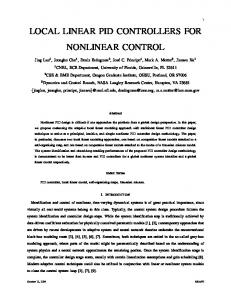
3.2.3 Proportional Derivative controller 𝑲𝒑
𝑦𝑠𝑝
+
𝑒(𝑡) +
-
𝑦(𝑡)
𝑢(𝑡) PLANT
𝑲𝒅
+
𝒅𝒆(𝒕) 𝒅𝒕
𝑦(𝑡) Figure 3.3: Proportional Derivative controller.
9
The Proportional Derivative controller actuating signal is related to the error by the equation [8, 51]: 𝑢(𝑡) = 𝐾𝑝 ∗ 𝑒(𝑡) + 𝐾𝑝 ∗ 𝑇𝐷
𝑑𝑒(𝑡) + 𝑐𝑠 . … … … … … … … … … (3.3) 𝑑𝑡
The Derivative time constant 𝑇𝐷 is an adjustable parameter. With the presence of derivative term the controller can anticipates, what the error will be in future and applies a control action which is proportional to the current rate of change in the error. The major drawback of derivative action includes: 1. For response with constant nonzero error it gives no control action since,
𝑑𝑒(𝑡) 𝑑𝑡
= 0.
2. For a noisy response with almost zero error, it can compute large derivatives and thus yield large action, although it is not needed. From Eq. (3.3), the transfer function of a proportional-derivative controller is given by: 𝐺𝑐 (𝑠) = 𝐾𝑝 (1 + 𝑇𝐷 𝑠).
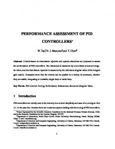
3.2.4 Proportional Integral Derivative controller 𝑲𝒑
𝑦𝑠𝑝
+
𝑒(𝑡)
𝒕
PLANT
𝑲𝒊 ∫ 𝒆(𝒕)𝒅𝒕 +
𝟎
-
𝑦(𝑡)
𝑢(𝑡)
+
𝑦(𝑡) 𝑲𝒅
𝒅𝒆(𝒕) 𝒅𝒕
Figure 3.4: Proportional Integral Derivative controller.
The output of the Proportional Integral Derivative controller is given by [20]: 𝑢(𝑡) = 𝐾𝑝 ∗ 𝑒(𝑡) +
𝐾𝑝 𝑡 𝑑𝑒(𝑡) ∫ 𝑒(𝑡) 𝑑𝑡 + 𝐾𝑝 ∗ 𝑇𝐷 + 𝑐𝑠 . … … … … … … … (3.4) 𝑇𝐼 0 𝑑𝑡
The Eq. (3.4) derives the transfer function of PID controller as: 𝐺𝑐 (𝑠) = 𝐾𝑝 (1 +
1 + 𝑇𝐷 𝑠). 𝑇𝐼 𝑠
The presence of integral control reduces the offset, but slows down the closed loop response of a process. To increase the speed of a closed loop response, the controller gain 10
𝐾𝑝 can be increased, but its increase may lead to a more oscillatory behavior and finally instability. The introduction of derivative mode brings stabilization effect to the system.
3.2.5 Proportional Integral Derivative controller with Derivative Kick correction If the process is under control and the outputs of the system are steady, then the error signal 𝑒(𝑡) = 𝑦𝑠𝑝 − 𝑦(𝑡) will be close to zero. Consider now the effect of a step change in the reference input 𝑦𝑠𝑝 .This will cause an immediate step change in 𝑒(𝑡) , and the controller will pass this step change directly into the controller output 𝑢(𝑡) , via the derivative term 𝐾𝑝 ∗ 𝑇𝐷
𝑑𝑒(𝑡) 𝑑𝑡
. Differentiating a step change will produce an impulse-like
spike in the control signal and this is termed as derivative kick. The very sharp spike-like change in the control signal will observed. This control signal could be driving a motor or a valve actuator device, and the kick could create serious problems for any electronic circuitry used in the device. If the derivative term is repositioned, so that the reference signal is not differentiated, then derivative kick is prevented. Therefore, in order to avoid derivative kick, the operation of the derivative term is performed on the measured process variable in place of an error signal. The implementation of conventional PID controller with derivative kick correction is shown in Fig. 3.5. The corresponding time domain equation of the PID controller after derivative kick correction is: 𝐾𝑝 𝑡 𝑑𝑦(𝑡) 𝑢(𝑡) = 𝐾𝑝 ∗ 𝑒(𝑡) + ∫ 𝑒(𝑡) 𝑑𝑡 − 𝐾𝑝 ∗ 𝑇𝐷 + 𝑐𝑠 . … … … … … … … (3.5) 𝑇𝐼 0 𝑑𝑡 The transfer function representation of Eq. (3.5) is: 𝑈𝑐 (𝑠) = 𝐾𝑝 (1 +
𝑦𝑠𝑝 +
𝑒 -
1 ) ∗ 𝐸(𝑠) − 𝐾𝑝 𝑇𝐷 ∗ 𝑠𝑌(𝑠). 𝑇𝐼 𝑠
𝑢𝑃𝐼
𝑢𝑃𝐼𝐷
PI +
-
𝑦 PLANT
𝑢𝐷 D
Figure 3.5: Proportional Integral Derivative controller with correction for derivative kick.
11
3.3 Conventional controllers’ tuning Ziegler-Nichols is the common method for tuning a conventional controller and widely popular in industries; it was introduced by John G. Ziegler and Nathaniel B. Nichols [35, 36]. In this tuning the “I” and “D” gains are first set to zero. The "P" gain is increased until it reaches the “Ultimate gain” 𝐾𝑢 at which the output of the closed loop starts to oscillate, at “Ultimate period” 𝑃𝑢 , their particular value are noted. Then 𝐾𝑢 & 𝑃𝑢 are used to set the PID family gains according to the relation given in Table 3.1. Table 3.1: Z-N based conventional controller tuning table. Gains Controllers
P PI
𝑲𝑷
𝑲𝑰
𝑲𝑫
0.5 ∗ 𝐾𝑢
-
-
0.455 ∗ 𝐾𝑢 0.545 ∗
PD*
0.71 ∗ 𝐾𝑢
PID
0.588 ∗ 𝐾𝑢
𝐾𝑢 𝑃𝑢
1.17 ∗
𝐾𝑢 𝑃𝑢
0.15 ∗ 𝑃𝑢 𝐾𝑢 ∗ 𝑃𝑢 13.6
* Not from the original Ziegler-Nichols Paper.
3.4 Conclusion Thus, the main focus of this chapter was only to make a general discussion on PID family controllers and Z-N method of tuning these controllers. -----------
12
CHAPTER-IV TYPE-1 FUZZY PID CONTROLLERS 4.1 Introduction Fuzzy logic controllers (FLC’s) are one of the useful control schemes for the plants having difficulties in deriving mathematical models, or having a performance limitations with conventional linear control schemes. Basically, all the approaches to the FLC’s design can be classified as follows [43]: 1) Expert systems approach, 2) Control engineering approach, 3) Intermediate approaches, 4) Combined approaches and synthetic approaches. The first approach originates from the methodology of expert systems. It is justified by consideration of an FLC system as an expert system, applied to problem-solving in control. In this approach, fuzzy sets are used to represent the knowledge or behavior of a control practitioner (an application expert or an operator) who may be acting only on subjective or intuitive knowledge. One should note that by using linguistic variables, fuzzy rules provide a natural framework for human thinking and knowledge formulation. Many experts find that fuzzy control rules present a convenient way to express their domain knowledge, so cooperation with the experts would be easier for a knowledge engineer. This approach was very popular in pioneering FLC design. In a purely expert approach, the choice of the structure, inputs, outputs and other parameters of a FLC system is the sole and solemn responsibility of the expert(s). Moreover, the supporters of this approach warn against further parameter modifications, pointing out that such adjustments can jeopardize an expert’s instructions. Changing the scaling factors and/or membership functions, for example, may result in losing the original linguistic sense of the rule base. The experts may not recognize their rules after tuning, and will then not be able to formulate new rules. Generally speaking, in this approach an expert system is designed. This expert system is specified for control applications and, after the design is completed, operates as a FLC. In this approach, any structure and set of the parameters of the FLC can be chosen. 13
Supporters of the control engineering approach consider the approach described above as too subjective and prone to errors, and try to make a choice on the basis of some objective criteria. This approach proposes to design a FLC by investigating, how the stability and performance indicators depends upon different FLC parameters. Thus, this approach clearly incorporates an analysis of FLC as one of the important stages of design. To evaluate a quality of such a FLC, the criteria commonly used in control engineering practice are applied. The control engineering approach allows traditional criteria to be applied in FLC design, and design methodologies to satisfy conventional design specifications to be developed, including parameters such as an overshoot, an integral and/or a steady-state error. Enhancing FLC engineering methods with an ability to learn, and the development of an adaptive FLC design, would significantly improve the quality of a FLC, making it much more robust and expanding its area of possible applications. Intermediate approaches proposes setting some of the parameters (e.g., membership functions) by the experts, and fixing the others (e.g., rules) with the methods inherited from control-system design. Combined approaches include an initial choice of the FLC structure and parameters, made by an expert, and further their adjustment performed using the control engineering methods. The development of these methods has led to the application of models, which computationally synthesize the properties of expert production systems, neural networks, and fuzzy logic. The application of a combined approach has come from control engineering practice. In a typical PID controller design for industry, the controller parameters are determined initially, and then later tuned manually to achieve the desired plant response. In this approach, manual tuning can be replaced with FLC supervision of a tuning process. The resulting improvements in the system response are accomplished by making on-line adjustments to the parameters of the FLC. It should be noted that an expert-systems approach was very popular at the beginning, though it is still being applied nowadays, of course in a modified way. Type-1 FLCs are both intuitive and numerical systems that map crisp inputs to a crisp output. The majority of them are knowledge-based in that they are described by fuzzy IFTHEN rules, which have to be established based on expert’s knowledge about the systems, controllers, performance, etc. In fuzzy control the introduction of input-output intervals and membership functions is more or less subjective, depending on the designer’s experience and knowledge about the plant, and the available information. However, it should be emphasized that after the determination of the fuzzy sets, all mathematics to 14
follow are rigorous. Also, the purpose of designing and applying fuzzy logic control systems is above all, to tackle those vague, ill-described and complex plants and processes that can hardly be handled by the classical systems theory, classical control techniques, and classical two-valued logic. In the present work Type-1 FLC was used to enhance the capability of Conventional PID controller family and control engineering approach was considered to design the Type-1 FLC. This chapter describes the design and tuning approach for various Type-1 Fuzzy Logic PID Controller’s.
4.2 Design principle of Fuzzy Logic Controller The block diagram of a Type-1 FLC is shown in Fig. 4.1. The main steps in designing the Type-1 FLC are:
Fuzzification.
Knowledge base establishment.
Inference engine.
Defuzzification module.
Knowledge base Input
Output Fuzzification
Inference engine
Defuzzification
ge Type-1 Fuzzy logic controller Deviation ge
ge
-
ge Plant or Process
Set point
+
Figure 4.1: Block diagram of Type-1 Fuzzy logic controller.
4.2.1 Fuzzification The process of fuzzification receives a normalized crisp input signal, and classifies it into membership functions. A grade of membership (a value between “0” and “1”), which measures the compatibility of the signal to the membership function, is assigned to the signal. Each membership function is identified by a linguistic variable like: Negative, Zero and Positive. The shapes of the membership functions are typically: Triangular, Trapezoidal, or Gaussian. In the present work, triangular membership function is used to 15
describe, three, five and seven linguistic variables. For example, Fig. 4.2(a) and Fig. 4.2(b) shows seven triangular membership functions for the error and change in error with fuzzy labels NB (Negative Big), NM (Negative Medium), NS (Negative Small), ZO (Zero), PS (Positive Small), PM (Positive Medium) and PB (Positive Big).
Figure 4.2: Triangular seven membership functions.
In the case of the triangular function shown in Fig. 4.2(a), the normalized Error signal (e) has membership in both the ZO and PS functions, while Fig. 4.2(b) show the Change in error signal (Δe) with membership in the NS and ZO functions. The values of points a and b represents the grade of membership of the Error in the ZO and PS functions, and the values of points c and d represent the grade of membership of the Change in error in the NS and ZO function. The sum of a and b, and the sum of c and d, will always be equal to one for triangular membership function [51]. In the present work, the physical values of actual inputs and output of the controller are mapped on the pre-determined normalized domain [-1, 1], so that input stays within the limits of membership function (avoid saturation). This mapping of input is called the normalization, and is done by so called normalization factor, whereas the output signal from the controller is denormalized in the output domain by the so called de-normalization factor. So that the control signal from the controller can be sufficient in magnitude to offer control action. The input family should contain a number of terms, designed such that the sum of membership values for each input is “1”. This can be achieved when the sets are triangular and cross their neighbor sets at the membership value: μ = 0.5, their peaks will be equidistant. Any input value can thus be a member of at most two sets, and its membership of each is a linear function of the input value.
4.2.2 Knowledge Base Establishment The knowledge base consists of a data base and a rule base. The data base provides information for the proper operation of fuzzification, inference, and defuzzification. This information consists of the input and output membership functions and other information 16
vital to the process logic of the FLC. The rule base is a collection of linguistic statements relating the input signals to the desired outputs. Designing a good fuzzy logic rule base is a key to obtain a satisfactory controller for a particular application. Classical analysis and control strategies should be incorporated in the establishment of a rule base. A general procedure in designing a fuzzy logic rule base is explained in the next paragraph. 𝑦(𝑡)
1
2
3
Region of control curve
𝑦𝑠𝑝
4
0
1. Positive e, Negative Δe. 2. Negative e, Negative Δe. 3. Negative e, Positive Δe. 4. Positive e, Positive Δe.
t Figure 4.3: Regions of a control curve.
Fig. 4.3, shows a set point tracking for a unit step input. The step response is divided into four general regions, each determined by the sign of the Error and Change in error. The regions are: Region 1: Positive Error, Negative Change in error. Region 2: Negative Error, Negative Change in error. Region 3: Negative Error, Positive Change in error. Region 4: Positive Error, Positive Change in error. A fifth region (resp. zero region) is used when both the Error and Change in error values are near zero or equal to zero (i.e., in steady state), and is not dependent on the sign of the signal. ̇ signal, is used to generate the Finally, the Error 𝑒(𝑡) signal and Change in error 𝑒(𝑡) control signal 𝑢(𝑡) from the controller, these two signals are defined by, 𝑒(𝑡) = 𝑦𝑠𝑝 − 𝑦(𝑡). ̇ = − 𝑦(𝑡) ̇ . 𝑒(𝑡) 17
The tracking Error signal 𝑒(𝑡) is an input variable to the controller. Oftentimes, one needs more auxiliary input variables in order to establish a complete and effective rule base. It can be easily seen that only the Error signal 𝑒(𝑡) is not enough to write an IF-THEN control rule. Indeed, suppose 𝑒(𝑡) > 0 at a moment. Then, 𝑒(𝑡) = 𝑦𝑠𝑝 − 𝑦(𝑡) > 0, or 𝑦𝑠𝑝 > 𝑦(𝑡), namely, at that moment the Process output 𝑦(𝑡) is below the set-point. This indicates that the Process output 𝑦(𝑡) lies either in region 1, or in region 4. However, this information is not sufficient for determining a control strategy that can bring the trajectory of 𝑦(𝑡) to approach the set-point thereafter: if the Process output 𝑦(𝑡) is in region 1 then the controller should take no action as the trajectory is going up; if the Process output 𝑦(𝑡) is in region 4, then the controller should accelerate the trajectory to the same moving direction (from pointing down to pointing up). Therefore, one more input variable that can distinguish these two situations is necessary. Same discussions apply to region 2 and region 3. Recall from calculus theory that if a curve is moving up then its derivative is positive, and if it is moving down then its derivative is negative. Hence, the Change of the ̇ or, ∆𝑒(𝑡), can help to distinguish the two situations lying in error signal, denoted as, 𝑒(𝑡) region 1 and 4, as well as that of region 2 and 3, shown in Fig. 4.3. Therefore use of Change of error as the second input variable for the Type-1 FLC controller is justified.
4.2.3 Inference Engine (If-Then Rule Base) A typical production of the rule base is of the form. IF (Process state) THEN (Control action). In the Fig. 4.3, it is clear that essentially one has four situations to consider: when Process output y(t) is at the situations represented by the four region 1, 2, 3, and 4. Thus needs atleast four rules for this set-point tracking application, in order to make it effectively work, one simple choice is: ̇ < 0 THEN Controller output 𝑢(𝑡) = Zero (System output is R1: IF 𝑒(𝑡) > 0 AND 𝑒(𝑡) approaching the input, no action is required by the controller). ̇ < 0 THEN Controller output 𝑢(𝑡) = Negative (System output is R2: IF 𝑒(𝑡) < 0 AND 𝑒(𝑡) going in wrong direction, negative action is required by the controller). ̇ > 0 THEN Controller output 𝑢(𝑡) = Zero (System output is R3: IF 𝑒(𝑡) < 0 AND 𝑒(𝑡) approaching the input, no action is required by the controller). ̇ > 0 THEN Controller output 𝑢(𝑡) = Positive (System output is R4: IF 𝑒(𝑡) > 0 AND 𝑒(𝑡) going in wrong direction, positive action is required by the controller).
18
Thus the rules R1, R2, R3 and R4 corresponds to the region 1, 2, 3, and 4, respectively, as shown in Fig. 4.3. It can be easily realized that by the above four rules, the controller is able to drive the process output y(t) to track the set-point 𝑦𝑠𝑝 . Therefore these four rules can be written in tabular form shown in Table 4.1. Table 4.1: Four rules in tabular form.
̇ 𝑒(𝑡)
N
P
N
Output is going in the wrong direction
Output is going in the right direction
P
Output is going in the right direction
Output is going in the wrong direction
𝑒(𝑡)
As the number of membership increases, more area of the curve shown in Fig. 4.3 will be considered for rule formation. Based on Table 4.1, rule base table for a 3-membership, 5membership and 7-membership function are shown in Table 4.2, 4.3 and 4.4, respectively, these rule base are used for designing FLC’s in the present work. Table 4.2: Rule-base for 3-membership function.
Δe e N Z P
N
Z
P
N N Z
N Z P
Z P P
Table 4.3: Rule-base for 5-membership function.
Δe e NB NS ZE PS PB
NB
NS
ZE
PS
PB
NB NB NS NS ZE
NB NS NS ZE PS
NS NS ZE PS PS
NS ZE PS PS PB
ZE PS PS PB PB
Table 4.4: Rule-base for 7-membership function.
Δe e NB NM NS ZE PS PM PB
NB
NM
NS
ZE
PS
PM
PB
NB NB NB NM NM NS ZE
NB NB NM NM NS ZE PS
NB NM NM NS ZE PS PM
NM NM NS ZE PS PM PM
NM NS ZE PS PM PM PB
NS ZE PS PM PM PB PB
ZE PS PM PM PB PB PB
19
The above method of rule-base production is called Mamdani inference engine. Mamdani fuzzy controller translates, directly, from external performance specifications and observations of the plant behavior to a rule-based linguistic control strategy. Mamdani assumed that there is no explicit plant model and/or no clear statement of the control design objectives. Informal knowledge of the operation of the given plant can be codified in terms of if-then rules, or condition-action rules, and form the basis for a linguistic control strategy. The basic form of Mamdani architecture is as follows: if OA1 is | and OA2 is | and ... then CA1 is | and CA2 is | ... where OA denotes observable attributes, and CA denotes controllable attributes.
4.2.4 Defuzzification module The defuzzification module is the reverse of the fuzzification module. It converts all the fuzzy terms created by the rule base of the controller to the crisp terms (numerical values), and then sends them to the physical system (plant, process), so as to execute the control of the physical system. Perhaps the most popular defuzzification method is the centroid calculation, which returns the center of area under the curve.
Figure 4.4: Centroid calculation return area under curve.
The crisp output value x (red line in Fig. 4.4) is the abscissa under the centre of gravity (COG) of the fuzzy set, 𝑢=
∑𝑖 𝜇(𝑥𝑖 ) ∗ 𝑥𝑖 ⁄∑ 𝜇(𝑥 ). 𝑖 𝑖
Here 𝑥𝑖 is a running point in a discrete universe, and 𝜇(𝑥𝑖 ), is its membership value in the membership function. The expression can be interpreted as the weighted average of the elements in the support set. For the continuous case, replace the summations by an
20
integrals. It is much used method although its computational complexity is relatively high. This method is also called centroid of area (COA).
4.3 Different types of Type-1 Fuzzy PID controllers’ Here Fuzzy logic is used to enhance the capabilities of a conventional PID controller. Different types of Type-1 Fuzzy PID controllers were considered for the study. The list of these controllers are given below. i.
Fuzzy Proportional controller.
ii.
Fuzzy Proportional Integral controller.
iii.
Fuzzy Proportional + Fuzzy Integral controller.
iv.
Fuzzy Proportional Derivative controller.
v.
Fuzzy Proportional + Fuzzy Integral + Fuzzy Derivative controller.
vi.
Fuzzy Proportional Integral + Digital Derivative controller.
vii.
Fuzzy Proportional Derivative + Digital Integral controller.
viii.
Fuzzy Proportional Integral + Fuzzy Proportional Derivative controller. Fuzzy P
Fuzzy P controller.
Fuzzy PD
Fuzzy PD controller
Fuzzy PI controller Type-1 Fuzzy PID controllers
Fuzzy PI Fuzzy P + Fuzzy I controller Fuzzy P + Fuzzy I + Fuzzy D controller. Fuzzy PI + Digital D controller. Fuzzy PID Fuzzy PD + Digital I controller. Fuzzy PI + Fuzzy PD controller.
Figure 4.5: Different member of Type-1 Fuzzy PID family controllers.
21
The block diagram of relationships between these controllers is shown in Fig. 4.5. The Fuzzy PID controllers mentioned from ‘v’ to ‘viii’ are mainly called hybrid Fuzzy PID controller. The main reason for constructing hybrid controller is that to implement a Fuzzy PID controller three input variables i.e., Error(𝑒), Derivative of error(∆𝑒) & Integral of error(∑ 𝑒) are required. But increasing the number of input variables causes a rise in the dimension of the rule table and, therefore, in the complexity of the system; this makes its implementation more complicated.
4.3.1 Fuzzy Proportional Controller A Conventional P controller is given by, 𝑢𝑃 (𝑡) = 𝐾𝑃 ∗ 𝑒(𝑡), … … … … … … … … … … … … … … (4.1) where 𝐾𝑃 is a Proportional gain. The discrete version of Eq. (4.1) is, 𝑢𝑃 (𝑘) = 𝐾𝑃 ∗ 𝑒(𝑘). … … … … … … … … … … … … … (4.2) The Z-transform of Eq. (4.2) is, 𝑈𝑃 (𝑧) = 𝐾𝑃 ∗ 𝐸(𝑧). … … … … … … … … … … … … … … (4.3) Thus this simple controller has one input 𝐸(𝑧) and one output 𝑈𝑃 (𝑧).
4.3.2 Fuzzy Proportional Integral Controller A classical PI controller is described by, 𝑡
𝑢𝑃𝐼 (𝑡) = 𝐾𝑃 ∗ 𝑒(𝑡) + 𝐾𝐼 ∗ ∫ 𝑒(𝑡) 𝑑𝑡. … … … … … … … … … … (4.4) 0
Differentiating Eq. (4.4), ̇ = 𝐾𝐼 ∗ 𝑒(𝑡) + 𝐾𝑃 ∗ 𝑒(𝑡) ̇ , … … … … … … … … … … … (4.5) 𝑢𝑃𝐼 (𝑡) where 𝐾𝑃 and 𝐾𝐼 are Proportional and Integral gains, respectively. The discrete version of Eq. (4.5) is, 𝑢𝑃𝐼 (𝑘) − 𝑢𝑃𝐼 (𝑘 − 1) 𝑒(𝑘) − 𝑒(𝑘 − 1) = 𝐾𝐼 ∗ 𝑒(𝑘) + 𝐾𝑃 ∗ [ ] . … … … … … (4.6) 𝑇𝑠 𝑇𝑠 Assume that 𝑇𝑠 = 1 sec in Eq. (4.6), the Z-transform of Eq. (4.6) will be, (1 − 𝑧 −1 )𝑈𝑃𝐼 (𝑧) = 𝐾𝐼 ∗ 𝐸(𝑧) + 𝐾𝑃 ∗ (1 − 𝑧 −1 )𝐸(𝑧). … … … … … (4.7) Eq. (4.7) can be written as ∆𝑈𝑃𝐼 (𝑧) = 𝐾𝐼 ∗ 𝐸(𝑧) + 𝐾𝑃 ∗ ∆𝐸(𝑧), … … … … … … … … … … (4.8) where, Incremental change in output is: ∆𝑈𝑃𝐼 (𝑧) = (1 − 𝑧 −1 )𝑈𝑃𝐼 (𝑧), and Change in error is: ∆𝐸(𝑧) = (1 − 𝑧 −1 )𝐸(𝑧). The Overall Fuzzy PI controller output will be, 𝑈𝑃𝐼 (𝑧) =
∆𝑈𝑃𝐼 (𝑧) … … … … … … … … … … … … … … (4.9) (1 − 𝑧 −1 ) 22
Thus, Fuzzy PI Controller based on Eq. (4.8) has two inputs: Error 𝐸(𝑧), and Change in error ∆𝐸(𝑧); and one output: ∆𝑈𝑃𝐼 (𝑧).
4.3.3 Fuzzy Proportional + Fuzzy Integral Controller The Fuzzy P + Fuzzy I controller can be obtained by adding Fuzzy P controller and Fuzzy I controller. It is based on an analytical expression given by Eq. (4.4). The Fuzzy P controller is already discussed in Section 4.3.1. The derivation of Fuzzy I controller is described below. A conventional Integral (I) controller is given by, 𝑡
𝑢𝐼 (𝑡) = 𝐾𝐼 ∗ ∫ 𝑒(𝑡) 𝑑𝑡 … … … … … … … … … … … … (4.10) 0
where 𝐾𝐼 is a Integral gain. The discrete version of Eq. (4.10) is given by, 𝑢𝐼 (𝑘) − 𝑢𝐼 (𝑘 − 1) = 𝐾𝐼 ∗ 𝑒(𝑘). … … … … … … … … … … (4.11) 𝑇𝑠 Assume that 𝑇𝑠 = 1 sec in Eq. (4.11), the Z-transform for Eq. (4.11) will be, (1 − 𝑧 −1 )𝑈𝐼 (𝑧) = 𝐾𝐼 ∗ 𝐸(𝑧). … … … … … … … … … … … (4.12) Let the incremental change in output from the Integral FLC be ∆𝑈𝐼 (𝑧), then from Eq. (4.12). ∆𝑈𝐼 (𝑧) = (1 − 𝑧 −1 )𝑈𝐼 (𝑧), or, 𝑈𝐼 (𝑧) =
1 ∗ ∆𝑈(𝑧), … … … … … … … … … … . (4.13) (1 − 𝑧 −1 )
The overall Fuzzy P + Fuzzy I controller can be obtain by algebraically summing Eq. (4.3) and Eq. (4.13). 𝑈𝑃+𝐼 (𝑧) = 𝑈𝑃 (𝑧) + 𝑈𝐼 (𝑧), … … … … … … … … … … … … … … (4.14) 𝑈𝑃+𝐼 (𝑧) = 𝐾𝑃 ∗ 𝐸(𝑧) +
1 𝐾 ∗ 𝐸(𝑧) … … … … … … … … … … (4.15) (1 − 𝑧 −1 ) 𝐼
This controller has two separate Inputs with Error 𝐸(𝑧), and one output 𝑈𝑃+𝐼 (𝑧).
4.3.4 Fuzzy Proportional Derivative controller A conventional PD controller is given by ̇ , . … … … … … … … … … (4.16) 𝑢𝑃𝐷 (𝑡) = 𝐾𝑃 ∗ 𝑒(𝑡) + 𝐾𝐷 ∗ 𝑒(𝑡) where 𝐾𝑃 and 𝐾𝐷 are Proportional and Derivative gains, respectively. The discrete version of Eq. (4.16) is:
23
𝑢𝑃𝐷 (𝑘) = 𝐾𝑃 ∗ 𝑒(𝑘) + 𝐾𝐷 ∗ [
𝑒(𝑘) − 𝑒(𝑘 − 1) ] , … … … … … … … … (4.17) 𝑇𝑠
Assume 𝑇𝑠 = 1 sec in Eq. (4.17), the Z-transform for Eq. (4.17) will be, 𝑈𝑃𝐷 (𝑧) = 𝐾𝑃 ∗ 𝐸(𝑧) + 𝐾𝐷 ∗ (1 − 𝑧 −1 )𝐸(𝑧), … … … … … … … … (4.18) Eq. (4.18) can be written in the form: 𝑈𝑃𝐷 (𝑧) = 𝐾𝑃 ∗ 𝐸(𝑧) + 𝐾𝐷 ∗ ∆𝐸(𝑧) … … … … … … … … … … (4.19) Where, Change in Error is ∆𝐸(𝑧) = (1 − 𝑧 −1 )𝐸(𝑧). Thus based on Eq. (4.19), Fuzzy PD Controller has two separate Input: Error 𝐸(𝑧), and Change in error: ∆𝐸(𝑧), and it has one output 𝑈𝑃𝐷 (𝑧).
4.3.5 Fuzzy Proportional + Fuzzy Integral + Fuzzy Derivative controller The Fuzzy P + Fuzzy I + Fuzzy D controller can be obtained by adding Fuzzy P controller, Fuzzy I controller and Fuzzy D controller. Fuzzy P and Fuzzy I controllers are discussed in Section 4.3.1 and 4.3.3, respectively. The derivation of Fuzzy D controller is given below. The conventional Derivative (D) controller is given by, 𝑢𝐷 (𝑡) = 𝐾𝐷 ∗ 𝑒̇ (𝑡). … … … … … … … … … … … … . (4.20) If the input signal is 𝑦𝑠𝑝 is constant, then. Where, 𝑒(𝑡) = 𝑦𝑠𝑝 − 𝑦(𝑡). Differentiating both side will give, ̇ = −𝑦(𝑡) ̇ … … … … … … … … … … … … … … … . (4.21) 𝑒(𝑡) ̇ in Eq. (4.20), will give, Substitute the value of 𝑒(𝑡) ̇ … … … … … … … … … … … … … (4.22) 𝑢𝐷 (𝑡) = −𝐾𝐷 ∗ 𝑦(𝑡) Thus, based on Eq. (4.22), the discrete form of Derivative (D) controller is expressed in terms of discrete output signal 𝑦(𝑘), in order to avoid the derivative kick. 𝑢𝐷 (𝑘) = −𝐾𝐷 ∗ [
𝑦(𝑘) − 𝑦(𝑘 − 1) ] , … … … … … … … … … (4.23) 𝑇𝑠
Assume 𝑇𝑠 = 1 sec in Eq. (4.23), the Z-transform for Eq. (4.23) will be. 𝑈𝐷 (𝑧) = −𝐾𝐷 ∗ (1 − 𝑧 −1 )𝑌(𝑧), … … … … … … … … … . (4.24) or, 𝑈𝐷 (𝑧) = −𝐾𝐷 ∗ ∆𝑌(𝑧), … … … … … … … … … … … (4.25) where, Change in Output is: ∆𝑌(𝑧) = (1 − 𝑧 −1 )𝑌(𝑧). The overall Fuzzy P + Fuzzy I + Fuzzy D, controller is obtain by algebraically summing the Eq. (4.3), Eq. (4.13) and Eq. (4.25), 24
𝑈𝑃+𝐼+𝐷 (𝑧) = 𝑈𝑃 (𝑧) + 𝑈𝐼 (𝑧) + 𝑈𝐷 (𝑧), … … … … … … … . . (4.26) 𝑈𝑃+𝐼+𝐷 (𝑧) = 𝐾𝑃 ∗ 𝐸(𝑧) +
1 𝐾 ∗ 𝐸(𝑧) − 𝐾𝐷 ∗ ∆𝑌(𝑧). … … . . . (4.27) (1 − 𝑧 −1 ) 𝐼
This controller has three separate Inputs in which two are Error 𝐸(𝑧) & one is change in output 𝛥𝑌(𝑧) and it has one output 𝑈𝑃+𝐼+𝐷 (𝑧).
4.3.6 Fuzzy Proportional Integral + Digital Derivative controller The Fuzzy PI + Digital D controller is obtained by adding Fuzzy PI controller and Digital D controller. The Fuzzy PI controller is discussed in Section 4.3.2. The derivation of Digital D controller follows as: The Discrete form of Derivative (D) controller is expressed in terms of output signal 𝑦(𝑘) in order to avoid the derivative kick. 𝑢𝐷𝐷 (𝑘) = −𝐾𝐷 ∗ [
𝑦(𝑘) − 𝑦(𝑘 − 1) ] , … … … … … … … … … (4.28) 𝑇𝑠
The Z-transform of Eq. (4.28) will be, 𝑈𝐷𝐷 (𝑧) = −𝐾𝐷 ∗ (1 − 𝑧 −1 )𝑌(𝑧). … … … … … … … … … (4.29) The overall Fuzzy PI + Digital D controller is obtain by algebraically summing the Eq. (4.8) and Eq. (4.29), 𝑈𝑃𝐼+𝐷𝐷 (𝑧) = 𝑈𝑃𝐼 (𝑧) + 𝑈𝐷𝐷 (𝑧). … … … … … … … … … (4.30) 𝑈𝑃𝐼+𝐷𝐷 (𝑧) =
1 [𝐾 ∗ 𝐸(𝑧) + 𝐾𝑃 ∗ ∆𝐸(𝑧)] − 𝐾𝐷 ∗ (1 − 𝑧 −1 )𝑌(𝑧) … … (4.31) (1 − 𝑧 −1 ) 𝐼
Fuzzy PI + Digital D controller has three separate Inputs: Error 𝐸(𝑧), and change in error 𝛥𝐸(𝑧)for Fuzzy PI controller, and 𝑌(𝑧) for Digital D controller; one output 𝑈𝑃𝐼+𝐷𝐷 (𝑧).
4.3.7 Fuzzy Proportional Derivative + Digital Integral controller The Fuzzy PD + Digital I controller is obtained by adding Fuzzy PD controller and Digital I controller. The Fuzzy PD controller is discussed in Section 4.3.4. The derivation of Digital I controller follows as: The Discrete form of Integral (I) is given by, 𝑢𝐷𝐼 (𝑘) − 𝑢𝐷𝐼 (𝑘 − 1) = 𝐾𝐼 ∗ 𝑒(𝑘). … … … … … … … … … (4.32) 𝑇𝑠 The Z-transform of Eq. (4.33) will be, (1 − 𝑧 −1 )𝑈𝐷𝐼 (𝑧) = 𝐾𝐷 ∗ 𝐸(𝑧). … … … … … … … … … … (4.33) Let the Incremental change in output from I controller be 𝛥𝑈𝐼 (𝑧) then, 𝛥𝑈𝐷𝐼 (𝑧) = (1 − 𝑧 −1 )𝑈𝐷𝐼 (𝑧), or, 25
𝑈𝐷𝐼 (𝑧) =
1 ∗ 𝛥𝑈𝐷𝐼 (𝑧), … … … … … … … . . … … . . (4.34) (1 − 𝑧 −1 )
The overall Fuzzy PD + Digital I controller is obtain by algebraically summing Eq. (4.19) and Eq. (4.35), 𝑈𝑃𝐷+𝐷𝐼 (𝑧) = 𝑈𝑃𝐷 (𝑧) + 𝑈𝐷𝐼 (𝑧), … … … … … … … … … … … … (4.35) 𝑈𝑃𝐷+𝐷𝐼 (𝑧) = 𝐾𝑃 ∗ 𝐸(𝑧) + 𝐾𝐷 ∗ ∆𝐸(𝑧) +
1 𝐾 ∗ 𝐸(𝑧) … … … … … … . . (4.36) (1 − 𝑧 −1 ) 𝐷
Fuzzy PD + Digital I controller has three separate inputs: Error 𝐸(𝑧) and change in error 𝛥𝐸(𝑧) for Fuzzy PD and error 𝐸(𝑧) for Digital Integral (I); one output 𝑈𝑃𝐷+𝐷𝐼 (𝑧).
4.3.8 Fuzzy Proportional Integral + Fuzzy Proportional Derivative controller The Fuzzy PI + Fuzzy PD controller is obtained by adding of Fuzzy PI controller and Fuzzy PD controller. The Fuzzy PI controller is discussed in Section 4.3.2, and Fuzzy PD controller is discussed in section 4.3.4. Thus based on Eq. (4.9) and Eq. (4.19), the output of Fuzzy PI + Fuzzy PD controller will be, 𝑈𝑃𝐼+𝑃𝐷 (𝑧) = 𝑈𝑃𝐼 (𝑧) + 𝑈𝑃𝐷 (𝑧), … … … … … … … … … … … (4.37) 𝑈𝑃𝐼+𝑃𝐷 (𝑧) =
1 [𝐾 ∗ 𝐸(𝑧) + 𝐾𝑃 ∗ ∆𝐸(𝑧)] + 𝐾𝑃 ∗ 𝐸(𝑧) + 𝐾𝐷 ∗ ∆𝐸(𝑧). … . . (4.38) (1 − 𝑧 −1 ) 𝐼
This controller has four inputs, out of which two are Error 𝐸(𝑧) and two are change in error 𝛥𝐸(𝑧). It has one output 𝑈𝑃𝐼+𝑃𝐷 (𝑧).
4.4 Tuning Type-1 Fuzzy PID controllers’ gain From the above study, it was observed that the equations of various Type-1 Fuzzy PID controllers is similar to the corresponding conventional PID controllers. Due to this relationship, the gains of Type-1 Fuzzy PID controllers i.e., GE, GCE, GCU & CU, were estimated in terms of conventional PID controller parameters i.e., gains 𝐾𝑝 , 𝐾𝑖 and 𝐾𝑑 [30, 31, 32].
4.4.1 Fuzzy Proportional controller 𝑒𝑛
𝐸𝑛 GE
FUZZY P CONTROLLER
Figure 4.6: Fuzzy P controller.
26
𝑢
𝑈𝑛 GU
The output 𝑈𝑛 from the Fuzzy P-controller is a non-linear function 𝑓 of input signal 𝑒𝑛 given by: 𝑈𝑛 = 𝑓(𝐺𝐸 ∗ 𝑒𝑛 ) ∗ 𝐺𝑈, where 𝐺𝐸 & 𝐺𝑈 are the fuzzy gains. The function 𝑓 is the fuzzy input-output map of the fuzzy controller. Using the linear approximation 𝑓(𝐺𝐸 ∗ 𝑒𝑛 ) = 𝐺𝐸 ∗ 𝑒𝑛 , then, 𝑈𝑛 = 𝐺𝑈 ∗ 𝐺𝐸 ∗ 𝑒𝑛 . … … … … … … … … … … … . (4.39) The discrete equation of conventional P controller is given by, 𝑈𝑛 = 𝐾𝑝 ∗ 𝑒𝑛 . … … … … … … … … … … … … … … . (4.40) Comparing Eq. (4.39) with Eq. (4.40), 𝐺𝑈 ∗ 𝐺𝐸 = 𝐾𝑝 … … … … … … … … … … … … … … (4.41) Assuming 𝐺𝐸 = 1 to avoid saturation, therefore, 𝐺𝑈 = 𝐾𝑝 … … … … … … … … … … … … … … … … (4.42) The value of 𝐺𝑈 can be known from 𝐾𝑝 .
4.4.2 Fuzzy Proportional Integral controller 𝑒𝑛
𝐸𝑛
GE
FUZZY PI CONTROLLER
𝐶𝐸𝑛
𝑐𝑒𝑛
𝑐𝑢
𝐶𝑈 GCU
𝟏 𝐒
𝑈𝑛
GCE Figure 4.7: Fuzzy PI controller.
The output 𝑈𝑛 from the Fuzzy PI-controller is a non-linear function 𝑓 of input signal 𝑒𝑛 and 𝑐𝑒𝑛 given by: 𝑈𝑛 = ∑𝑛𝑖=1[𝑓(𝐺𝐸 ∗ 𝑒𝑖 , 𝐺𝐶𝐸 ∗ 𝑐𝑒𝑖 ) ∗ 𝐺𝐶𝑈] ∗ 𝑇𝑠 . Where, 𝐺𝐸, 𝐺𝐶𝐸 & 𝐺𝐶𝑈 are the fuzzy gains. The function 𝑓 is the fuzzy input-output map of the fuzzy controller. Using the linear approximation 𝑓(𝐺𝐸 ∗ 𝑒𝑖 , 𝐺𝐶𝐸 ∗ 𝑐𝑒𝑖 ) = 𝐺𝐸 ∗ 𝑒𝑖 + 𝐺𝐶𝐸 ∗ 𝑐𝑒𝑖 then, 𝑛
𝑈𝑛 = ∑( 𝐺𝐸 ∗ 𝑒𝑖 + 𝐺𝐶𝐸 ∗ 𝑐𝑒𝑖 ) ∗ 𝐺𝐶𝑈 ∗ 𝑇𝑠 , … … … … … … … (4.43) 𝑖=1
where, 𝑐𝑒𝑖 =
𝑒𝑖 −𝑒𝑖−1 𝑇𝑠
.
= 𝐺𝐶𝑈 ∗ [𝐺𝐸 ∗ ∑𝑛𝑖=1 𝑒𝑖 ∗ 𝑇𝑠 + 𝐺𝐶𝐸 ∗ ∑𝑛𝑖=1(𝑒𝑖 − 𝑒𝑖−1 )], 𝑛
𝐺𝐸 = 𝐺𝐶𝐸 ∗ 𝐺𝐶𝑈 ∗ [ ∗ ∑ 𝑒𝑖 ∗ 𝑇𝑠 + 𝑒𝑛 ] , … … … . . … … … … … . . (4.44) 𝐺𝐶𝐸 𝑖=1
On comparing Eq. (4.44) with the discrete approximation of conventional PI controller given by Eq. (4.45), 27
𝑛
1 𝑢𝑛 = 𝐾𝑝 (𝑒𝑛 + ∑ 𝑒𝑗 ∗ 𝑇𝑠 ) … … … … … … … … … … (4.45) 𝑇𝐼 𝑗=1
Following equations can be obtained: 𝐺𝐶𝐸 ∗ 𝐺𝐶𝑈 = 𝐾𝑝 … … … … … … … … … … … … … (4.46) 𝐺𝐸 ⁄𝐺𝐶𝐸 = 1⁄𝑇𝐼 . … … … … … … … … … … … … . (4.47) Assuming 𝐺𝐸 = 1 in Eq. (4.47) to avoid saturation, therefore: 𝐺𝐶𝐸 = 𝑇𝐼 … … … … … … … … … … … … … . . . (4.48) 𝐺𝐶𝑈 = 𝐾𝐼 , … … … … … … … … … … … … … . . (4.49) where, 𝐾𝐼 = 𝐾𝑝 ⁄𝑇𝐼 . The value of 𝐺𝐶𝐸 & 𝐺𝐶𝑈 can be calculated in term of 𝐾𝑝 & 𝑇𝐼 .
4.4.3 Fuzzy Proportional + Fuzzy Integral controller 𝑒𝑛
𝐸𝑛 GE
𝑈𝑛 𝑐𝑢
FUZZY I
GE
𝑈𝑃 GU
CONTROLLER 𝐸𝑛
𝑒𝑛
𝑢
FUZZY P
𝐶𝑈 GCU
CONTROLLER
𝟏 𝐒
𝑈𝐼
Figure 4.8: Fuzzy P + Fuzzy I controller.
The output 𝑈𝑛 from the Fuzzy P + Fuzzy I controller is a non-linear function 𝑓1 and 𝑓2 of input signal 𝑒𝑛 given by, 𝑈𝑛 = ∑𝑛𝑖=1[𝑓1 (𝐺𝐸 ∗ 𝑒𝑖 ) ∗ 𝐺𝐶𝑈] ∗ 𝑇𝑠 + 𝑓2 (𝐺𝐸 ∗ 𝑒𝑛 ) ∗ 𝐺𝑈. Where, 𝐺𝐸, 𝐺𝑈 & 𝐺𝐶𝑈 are the fuzzy gains. The function 𝑓1 & 𝑓2 is the fuzzy input-output map of the fuzzy controllers. Using the linear approximation 𝑓1 (𝐺𝐸 ∗ 𝑒𝑖 ) = 𝐺𝐸 ∗ 𝑒𝑖 and 𝑓2 (𝐺𝐸 ∗ 𝑒𝑛 ) = 𝐺𝐸 ∗ 𝑒𝑛 then, 𝑛
𝑈𝑛 = ∑[(𝐺𝐸 ∗ 𝑒𝑖 ) ∗ 𝐺𝐶𝑈] ∗ 𝑇𝑠 + (𝐺𝐸 ∗ 𝑒𝑛 ) ∗ 𝐺𝑈, … … … … . (4.50) 𝑖=1 𝑛
𝑛
= 𝐺𝐶𝑈 ∗ ∑ 𝐺𝐸 ∗ 𝑒𝑖 ∗ 𝑇𝑠 + 𝐺𝑈 ∗ 𝐺𝐸 ∗ 𝑒𝑛 = 𝐺𝐶𝑈 ∗ 𝐺𝐸 ∗ ∑ 𝑒𝑖 ∗ 𝑇𝑠 + 𝐺𝑈 ∗ 𝐺𝐸 ∗ 𝑒𝑛 , 𝑖=1
𝑖=1 𝑛
= 𝐺𝑈 ∗ 𝐺𝐸 ∗ [
𝐺𝐶𝑈 ∑ 𝑒𝑖 ∗ 𝑇𝑠 + 𝑒𝑛 ] , … … … … … … … … … (4.51) 𝐺𝑈 𝑖=1
On comparing, Eq. (4.51) with the discrete approximation of a conventional PI controller given by Eq. (4.45), following equations are obtained: 𝐺𝐸 ∗ 𝐺𝑈 = 𝐾𝑝 , … … … … … … … … … … … … … … (4.52) 28
𝐺𝐶𝑈⁄𝐺𝑈 = 1⁄𝑇𝐼 . … … … … … … … … … … … … . . (4.53) Assuming 𝐺𝐸 = 1 in Eq. (4.52) to avoid saturation. 𝐺𝑈 = 𝐾𝑝 … … … … … … … … … … … … … … … . . (4.54) 𝐺𝐶𝑈 = 𝐾𝐼 … … … … … … … … … … … … … … . . (4.55) where 𝐾𝐼 = 𝐾𝑝 ⁄𝑇𝐼 . The value of 𝐺𝑈 & 𝐺𝐶𝑈 can be calculated in term of 𝐾𝑝 & 𝑇𝐼 .
4.4.4 Fuzzy Proportional Derivative controller 𝑒𝑛
𝐸𝑛
GE
FUZZY PD 𝐶𝐸𝑛
𝑐𝑒𝑛
GCE
𝑢
CONTROLLER
𝑈𝑛 GU
Figure 4.9: Fuzzy PD controller.
The output 𝑈𝑛 from the Fuzzy PD-controller is a non-linear function 𝑓 of input signal 𝑒𝑛 & 𝑐𝑒𝑛 given by, 𝑈𝑛 = 𝑓(𝐺𝐸 ∗ 𝑒𝑛 , 𝐺𝐶𝐸 ∗ 𝑐𝑒𝑛 ) ∗ 𝐺𝑈. Where, 𝐺𝐸, 𝐺𝐶𝐸 & 𝐺𝑈 are the fuzzy gains. The function 𝑓 is the fuzzy input-output map of the fuzzy controller. Using the linear approximation 𝑓(𝐺𝐸 ∗ 𝑒𝑛 , 𝐺𝐶𝐸 ∗ 𝑐𝑒𝑛 ) = 𝐺𝐸 ∗ 𝑒𝑛 + 𝐺𝐶𝐸 ∗ 𝑐𝑒𝑛 then, 𝑈𝑛 = (𝐺𝐸 ∗ 𝑒𝑛 + 𝐺𝐶𝐸 ∗ 𝑐𝑒𝑛 ) ∗ 𝐺𝑈, … … … . . … … … … . . (4.56) = 𝐺𝐸 ∗ 𝐺𝑈 ∗ [ where, 𝑐𝑒𝑛 =
𝑒𝑛 −𝑒𝑛−1 𝑇𝑠
𝐺𝐶𝐸 ∗ 𝑐𝑒𝑛 + 𝑒𝑛 ] , … … … … … … … … . (4.57) 𝐺𝐸
. On comparing the Eq. (4.57) with the discrete approximation of
conventional PD controller given by Eq. (4.58). 𝑢𝑛 = 𝐾𝑝 (𝑒𝑛 + 𝑇𝑑 ∗
𝑒𝑛 − 𝑒𝑛−1 ) , … … … … … … … … … (4.58) 𝑇𝑠
Following equations are obtained: 𝐺𝐸 ∗ 𝐺𝑈 = 𝐾𝑝 , … … … … … … … … … … … … . (4.59) 𝐺𝐶𝐸 ⁄𝐺𝐸 = 𝑇𝑑 , … … … … … … … … … … … … … (4.60) Assuming 𝐺𝐸 = 1 in Eq. (4.59) to avoid saturation. 𝐺𝑈 = 𝐾𝑝 … … … … … … … … … … … … . . … … . (4.61) 𝐺𝐶𝐸 = 𝑇𝑑 … … … … … … … … … … … … … … … (4.62) The value of 𝐺𝐶𝐸 & 𝐺𝑈 can be calculated in term of 𝐾𝑝 and 𝑇𝑑 .
4.4.5 Fuzzy Proportional + Fuzzy Integral + Fuzzy Derivative controller The output 𝑈𝑛 from the Fuzzy P + Fuzzy I + Fuzzy D controller is a non-linear function 𝑓1 , 𝑓2 & 𝑓3 of input signals 𝑒𝑛 , 𝑐𝑒𝑛 and 𝑐𝑦𝑛 given by, 29
𝑈𝑛 = 𝑓1 (𝐺𝐸 ∗ 𝑒𝑛 ) ∗ 𝐺𝑈 + ∑𝑛𝑖=1[𝑓2 (𝐺𝐸 ∗ 𝑒𝑖 ) ∗ 𝐺𝐶𝑈] ∗ 𝑇𝑠 − 𝑓3 (𝐺𝐶𝐸 ∗ 𝑐𝑦𝑛 ) ∗ 𝐺𝑈. 𝐸𝑛
𝑒𝑛 GE
GU
CONTROLLER
𝑒𝑛
𝐸𝑛 GE
𝑐𝑢
FUZZY I
−𝐶𝑌𝑛 GCE
𝐶𝑈 GCU
CONTROLLER
−𝑐𝑦𝑛
𝑈𝑃
𝑢
FUZZY P
𝑈𝐼 𝟏 𝐒 𝑈𝐷
𝑢
FUZZY D CONTROLLER
𝑈𝑛
GU
Figure 4.10: Fuzzy P + Fuzzy I + Fuzzy D controller.
Where, 𝐺𝐸, 𝐺𝐶𝐸, 𝐺𝐶𝑈 & 𝐺𝑈 are the fuzzy gains. The function 𝑓1 , 𝑓2 and 𝑓3 are the fuzzy input-output map of the fuzzy controllers. Using the linear approximation:𝑓1 (𝐺𝐸 ∗ 𝑒𝑛 ) = 𝐺𝐸 ∗ 𝑒𝑛 and 𝑓2 (𝐺𝐸 ∗ 𝑒𝑖 ) = 𝐺𝐸 ∗ 𝑒𝑖 and 𝑓3 (𝐺𝐶𝐸 ∗ 𝑐𝑦𝑛 ) = 𝐺𝐶𝐸 ∗ 𝑐𝑦𝑛 , then, 𝑛
𝑈𝑛 = 𝐺𝑈 ∗ 𝐺𝐸 ∗ 𝑒𝑛 + ∑(𝐺𝐸 ∗ 𝐺𝐶𝑈 ∗ 𝑒𝑖 ) ∗ 𝑇𝑠 − 𝐺𝑈 ∗ 𝐺𝐶𝐸 ∗ 𝑐𝑦𝑛 , … . . (4.63) 𝑖=1
= 𝐺𝑈 ∗ 𝐺𝐸 ∗ 𝑒𝑛 + 𝐺𝐶𝑈 ∗ 𝐺𝐸 ∗ ∑𝑛𝑖=1(𝑒𝑖 ∗ 𝑇𝑠 ) − 𝐺𝑈 ∗ 𝐺𝐶𝐸 ∗ 𝑐𝑦𝑛 , 𝑛
𝐺𝐶𝑈 𝐺𝐶𝐸 = 𝐺𝑈 ∗ 𝐺𝐸 [𝑒𝑛 + ∗ ∑(𝑒𝑖 ∗ 𝑇𝑠 ) − ∗ 𝑐𝑦𝑛 ] . … … … … … … … (4.64) 𝐺𝑈 𝐺𝐸 𝑖=1
On comparing Eq. (4.64) with the discrete approximation of conventional PID controller given by Eq. (4.65). 𝑛
1 𝑦𝑛 − 𝑦𝑛−1 𝑢𝑛 = 𝐾𝑝 ( 𝑒𝑛 + ∗ ∑ 𝑒𝑗 ∗ 𝑇𝑠 − 𝑇𝑑 ∗ ) , … … … … … … (4.65) 𝑇𝐼 𝑇𝑠 𝑗=1
Following equations are obtained: 𝐺𝐸 ∗ 𝐺𝑈 = 𝐾𝑝 , … … … … … … … … … … … … … (4.66) 𝐺𝐶𝑈⁄𝐺𝑈 = 1⁄𝑇 , … … … … . … … … … … … … … . (4.67) 𝐺𝐶𝐸 ⁄𝐺𝐸 = 𝑇𝑑 , … … … . … . … … … … … … … … (4.68) Assuming 𝐺𝐸 = 1 in Eq. (4.66) to avoid saturation. 𝐺𝑈 = 𝐾𝑝 … … … … . … … … . … … … … … … … . (4.69) 𝐺𝐶𝑈 = 𝐾𝐼 … … … … … … … … … … … … … … … (4.70) 𝐺𝐶𝐸 = 𝑇𝑑 … … … … … … … … … … … … … … … (4.71) where 𝐾𝐼 = 𝐾𝑝 ⁄𝑇𝐼 . The value of 𝐺𝐶𝐸, 𝐺𝐶𝑈 & 𝐺𝑈 can be calculated in term of 𝐾𝑝 , 𝑇𝐼 , and 𝑇𝑑 . 30
4.4.6 Fuzzy Proportional Integral + Digital Derivative controller 𝐸𝑛
𝑒𝑛 GE
FUZZY PI 𝐶𝐸𝑛
𝑐𝑒𝑛 GCE −𝑐𝑦𝑛
𝐶𝑈
𝑐𝑢
CONTROLLER
GCU
−𝐶𝑌𝑛
𝟏 𝐒
𝑈𝑃𝐼 𝑈𝑛
𝑈𝐷𝐷
GDE Figure 4.11: Fuzzy PI + Digital D controller.
The output 𝑈𝑛 from the Fuzzy PI + D controller is a non-linear function 𝑓 of input signal 𝑒𝑛 and 𝑐𝑒𝑛 , and sum of signal, − 𝑐𝑦𝑛 given by. 𝑈𝑛 = ∑𝑛𝑖=1[𝑓(𝐺𝐸 ∗ 𝑒𝑖 , 𝐺𝐶𝐸 ∗ 𝑐𝑒𝑖 ) ∗ 𝐺𝐶𝑈] ∗ 𝑇𝑠 − 𝐺𝐷𝐸 ∗ 𝑐𝑦𝑛 . Where, 𝐺𝐸, 𝐺𝐶𝐸, 𝐺𝐶𝑈 & 𝐺𝐷𝐸 are the fuzzy gains. The function 𝑓 is the fuzzy inputoutput map of the fuzzy controller. Using the linear approximation, 𝑓(𝐺𝐸 ∗ 𝑒𝑖 , 𝐺𝐶𝐸 ∗ 𝑐𝑒𝑖 ) = 𝐺𝐸 ∗ 𝑒𝑖 + 𝐺𝐶𝐸 ∗ 𝑐𝑒𝑖 then, 𝑛
𝑈𝑛 = ∑( 𝐺𝐸 ∗ 𝑒𝑖 + 𝐺𝐶𝐸 ∗ 𝑐𝑒𝑖 ) ∗ 𝐺𝐶𝑈 ∗ 𝑇𝑠 − 𝐺𝐷𝐸 ∗ 𝑐𝑦𝑛 , … … … … (4.72) 𝑖=1
where 𝑐𝑦𝑛 =
𝑦𝑛− 𝑦𝑛−1 𝑇𝑠
.
= 𝐺𝐶𝑈 ∗ 𝐺𝐸 ∗ ∑𝑛𝑖=1 𝑒𝑖 ∗ 𝑇𝑠 + 𝐺𝐶𝑈 ∗ 𝐺𝐶𝐸 ∗ ∑𝑛𝑖=1 𝑒𝑖 − 𝑒𝑖−1 − 𝐺𝐷𝐸 ∗ 𝑐𝑦𝑛 . 𝑛
𝐺𝐸 𝐺𝐷𝐸 = 𝐺𝐶𝑈 ∗ 𝐺𝐶𝐸 [𝑒𝑛 + ∗ ∑ 𝑒𝑖 ∗ 𝑇𝑠 − ∗ 𝑐𝑦𝑛 ] , … … … … (4.73) 𝐺𝐶𝐸 𝐺𝐶𝑈 ∗ 𝐺𝐶𝐸 𝑖=1
On comparing Eq. (4.73) with the discrete approximation of conventional PID controller given by Eq. (4.65); the following set of equations are obtained: 𝐺𝐶𝑈 ∗ 𝐺𝐶𝐸 = 𝐾𝑝 , … … … … … … … … … … … … … (4.74) 𝐺𝐷𝐸 ⁄(𝐺𝐶𝑈 ∗ 𝐺𝐶𝐸) = 𝑇𝑑 , … … … … … … … … … … … (4.75) 𝐺𝐸 ⁄𝐺𝐶𝐸 = 1⁄𝑇𝐼 , … … … … … … … … … … … … … (4.76) Assuming 𝐺𝐸 = 1 in Eq. (4.77) to avoid saturation, then, 𝐺𝐶𝐸 = 𝑇𝐼 , … … … … … … … … … … … … … … … (4.77) 𝐺𝐶𝑈 = 𝐾𝐼 , … … … … . … … … . … … … … … … … (4.78) 𝐺𝐷𝐸 = 𝐾𝐷 , … … … … … … … … … … … . … … … . (4.79) where 𝐾𝐼 = 𝐾𝑝 ⁄𝑇𝐼 and 𝐾𝐷 = 𝐾𝑝 ∗ 𝑇𝐼 . The value of 𝐺𝐶𝐸, 𝐺𝐶𝑈 & 𝐺𝐷𝐸 can be calculated in term of 𝐾𝑝 , 𝑇𝐼 and 𝑇𝑑 .
31
4.4.7 Fuzzy Proportional Derivative + Digital Integral controller 𝑒𝑛
𝐸𝑛 GE
𝑐𝑒𝑛 GCE
𝑈𝑃𝐷
FUZZY PD 𝐶𝐸𝑛
CONTROLLER
𝑢
𝑈𝑛 GU
𝑈𝐷𝐼
𝐼𝐸𝑛
𝑖𝑒𝑛 GIE
Figure 4.12: Fuzzy PD + Digital I controller.
The output 𝑈𝑛 from the Fuzzy PD + I controller is a non-linear function 𝑓 of input signal 𝑒𝑛 & 𝑐𝑒𝑛 and sum of signal 𝑖𝑒𝑛 given by, 𝑈𝑛 = 𝑓(𝐺𝐸 ∗ 𝑒𝑛 , 𝐺𝐶𝐸 ∗ 𝑐𝑒𝑛 ) ∗ 𝐺𝑈 + 𝐺𝐼𝐸 ∗ 𝑖𝑒𝑛 ∗ 𝐺𝑈. Where, 𝑖𝑒𝑛 = ∑𝑛𝑖=1 𝑒𝑖 ∗ 𝑇𝑠 and, 𝐺𝐸, 𝐺𝐶𝐸, 𝐺𝑈 & 𝐺𝐼𝐸 are the fuzzy gains. The function 𝑓 is the fuzzy input-output map of the fuzzy controller. Using the linear approximation𝑓(𝐺𝐸 ∗ 𝑒𝑛 , 𝐺𝐶𝐸 ∗ 𝑐𝑒𝑛 ) = 𝐺𝐸 ∗ 𝑒𝑛 + 𝐺𝐶𝐸 ∗ 𝑐𝑒𝑛 then, 𝑈𝑛 = [𝐺𝐸 ∗ 𝑒𝑛 + 𝐺𝐶𝐸 ∗ 𝑐𝑒𝑛 + 𝐺𝐼𝐸 ∗ 𝑖𝑒𝑛 ] ∗ 𝐺𝑈, … … … … … … … (4.80) where 𝑐𝑒𝑛 =
𝑒𝑛 −𝑒𝑛−1 𝑇𝑠
. = 𝐺𝐸 ∗ 𝐺𝑈 ∗ [ 𝑒𝑛 +
𝐺𝐼𝐸 𝐺𝐶𝐸 ∗ 𝑖𝑒𝑛 + ∗ 𝑐𝑒𝑛 ] , … … … … … … … (4.81) 𝐺𝐸 𝐺𝐸
On comparing the Eq. (4.81) with the discrete approximation of conventional PID controller given by Eq. (4.82): 𝑛
1 𝑒𝑛 − 𝑒𝑛−1 𝑢𝑛 = 𝐾𝑝 ( 𝑒𝑛 + ∗ ∑ 𝑒𝑗 ∗ 𝑇𝑠 + 𝑇𝑑 ∗ ) , … … … … … (4.82) 𝑇𝐼 𝑇𝑠 𝑗=1
Following sets of equation are obtained: 𝐺𝐸 ∗ 𝐺𝑈 = 𝐾𝑝 , … … . … … … … … … … … … … … . . (4.83) 𝐺𝐶𝐸 = 𝑇𝑑 , … … … … … … … … … … … … … … … … . (4.84) 𝐺𝐸 𝐺𝐼𝐸 1 = , … … . … … … … … … … … … … … … … … (4.85) 𝐺𝐸 𝑇𝐼 Assuming 𝐺𝐸 = 1 in Eq. (4.83) to avoid saturation, then, 𝐺𝑈 = 𝐾𝑝 , … … … … … … … … … … … … … … … … (4.86) 𝐺𝐶𝐸 = 𝑇𝑑 , … … … … … … … … … … … … … … … … (4.87) 𝐺𝐼𝐸 = 1⁄𝑇𝐼 . … … … … … … … … … … … … … … … … (4.88) The value of 𝐺𝐶𝐸, 𝐺𝑈 and 𝐺𝐼𝐸 can be calculated in term of 𝐾𝑝 , 𝑇𝐼 and 𝑇𝑑 . 32
4.4.8 Fuzzy Proportional Integral + Fuzzy Proportional Derivative controller 𝑒𝑛
GE
𝐸𝑛 𝐶𝐸𝑛
𝑐𝑒𝑛 GCE GE 𝑐𝑒𝑛
𝐶𝐸𝑛 GCE
GCU
CONTROLLER
𝐸𝑛
𝑒𝑛
𝐶𝑈
𝑐𝑢
FUZZY PI
CONTROLLER
𝑈𝑃𝐼 𝑈𝑛
𝑈𝑃𝐷
𝑢
FUZZY PD
𝟏 𝐒
GU
Figure 4.13: Fuzzy PI + Fuzzy PD controller.
The output 𝑈𝑛 from the Fuzzy PI + Fuzzy PD controller is a non-linear function 𝑓1 & 𝑓2 of input signal 𝑒𝑛 & 𝑐𝑒𝑛 given by, 𝑈𝑛 = ∑𝑛𝑖=1[𝑓1 (𝐺𝐸 ∗ 𝑒𝑖 , 𝐺𝐶𝐸 ∗ 𝑐𝑒𝑖 ) ∗ 𝐺𝐶𝑈] ∗ 𝑇𝑠 + 𝑓2 (𝐺𝐸 ∗ 𝑒𝑛 , 𝐺𝐶𝐸 ∗ 𝑐𝑒𝑛 ) ∗ 𝐺𝑈. Where, 𝐺𝐸 , 𝐺𝐶𝐸 , 𝐺𝐶𝑈 & 𝐺𝑈 are the fuzzy gains. The function 𝑓1 and 𝑓2 is the fuzzy input-output map of the fuzzy controllers. Using the linear approximation: 𝑓1 (𝐺𝐸 ∗ 𝑒𝑛 , 𝐺𝐶𝐸 ∗ 𝑐𝑒𝑛 ) = 𝐺𝐸 ∗ 𝑒𝑛 + 𝐺𝐶𝐸 ∗ 𝑐𝑒𝑛 and 𝑓2 (𝐺𝐸 ∗ 𝑒𝑛 , 𝐺𝐶𝐸 ∗ 𝑐𝑒𝑛 ) = 𝐺𝐸 ∗ 𝑒𝑛 + 𝐺𝐶𝐸 ∗ 𝑐𝑒𝑛 then, 𝑛
𝑈𝑛 = ∑( 𝐺𝐸 ∗ 𝑒𝑖 + 𝐺𝐶𝐸 ∗ 𝑐𝑒𝑖 ) ∗ 𝐺𝐶𝑈 ∗ 𝑇𝑠 + [𝐺𝐸 ∗ 𝑒𝑛 + 𝐺𝐶𝐸 ∗ 𝑐𝑒𝑛 ] ∗ 𝐺𝑈, … … (4.89) 𝑖=1
= 𝐺𝐶𝑈 ∗ [𝐺𝐸 ∗ ∑𝑛𝑖=1 𝑒𝑖 ∗ 𝑇𝑠 + 𝐺𝐶𝐸 ∗ ∑𝑛𝑖=1(𝑒𝑖 − 𝑒𝑖−1 )] + 𝐺𝑈 ∗ [𝐺𝐸 ∗ 𝑒𝑛 + 𝐺𝐶𝐸 ∗ 𝑐𝑒𝑛 ]. = (𝐺𝑈 ∗ 𝐺𝐸 + 𝐺𝐶𝐸 ∗ 𝐺𝐶𝑈 ) ∗ 𝑒𝑛 + 𝐺𝐶𝑈 ∗ 𝐺𝐸 ∗ ∑𝑛𝑖=1 𝑒𝑖 ∗ 𝑇𝑠 + 𝐺𝐶𝐸 ∗ 𝐺𝑈 ∗ 𝑐𝑒𝑛 . Let, 𝐺𝑈 ∗ 𝐺𝐸 + 𝐺𝐶𝐸 ∗ 𝐺𝐶𝑈 = 𝐾, then, 𝑛
𝐺𝐶𝑈 ∗ 𝐺𝐸 𝐺𝐶𝐸 ∗ 𝐺𝑈 = 𝐾 ∗ [𝑒𝑛 + ∗ ∑(𝑒𝑖 ∗ 𝑇𝑠 ) + ∗ 𝑐𝑒𝑛 ] . … … … … … (4.90) 𝐾 𝐾 𝑖=1
On comparing, Eq. (4.90) with the discrete approximation of PID controller given by Eq. (4.82), the following sets of equation are obtained [47]: 𝐾 = 𝐾𝑝 , 𝐺𝑈 ∗ 𝐺𝐸 + 𝐺𝐶𝐸 ∗ 𝐺𝐶𝑈 = 𝐾𝑝 … … … … … … … … … … … (4.91) 𝐾𝑝 𝐺𝐶𝑈 ∗ 𝐺𝐸 1 = ≡ 𝐺𝐶𝑈 ∗ 𝐺𝐸 = = 𝐾𝐼 , … … … … … … … . (4.92) 𝐾 𝑇𝐼 𝑇𝐼 𝐺𝐶𝐸 ∗ 𝐺𝑈 = 𝑇𝑑 ≡ 𝐺𝐶𝐸 ∗ 𝐺𝑈 = 𝐾𝑝 ∗ 𝑇𝑑 = 𝐾𝑑 . … … … … . . (4.93) 𝐾 If 𝛼 and 𝛽 = 1 − 𝛼 are the two variable, then 𝐾𝑝 be written as, (1 − 𝛼) ∗ 𝐾𝑝 + 𝛼 ∗ 𝐾𝑝 = 𝐾𝑝 , or, 𝛽 ∗ 𝐾𝑝 + 𝛼 ∗ 𝐾𝑝 = 𝐾𝑝 , … … … … … (4.94) 33
On comparing Eq. (4.94) with Eq. (4.91), following relations are obtained. 𝐺𝐶𝐸 ∗ 𝐺𝐶𝑈 = 𝛼 ∗ 𝐾𝑝 , … … … … … … … … … … … … . . (4.95) 𝐺𝑈 ∗ 𝐺𝐸 = 𝛽 ∗ 𝐾𝑝 , … … … … … … … … … … … … … (4.96) Assuming 𝐺𝐸 = 1 in Eq. (4.96) to avoid saturation. Eq. (4.96) will become, 𝐺𝑈 = 𝛽 ∗ 𝐾𝑝 , … … … … … … … … … … … . . … … … (4.97) Eq. (4.92) will become, 𝐺𝐶𝑈 = 𝐾𝐼 , … … … … … … … … … … … … … … … . . (4.98) Eq. (4.93) will become, 𝐺𝐶𝐸 =
𝐾𝑑 , … … … … … … … … … … … . . (4.99) (1 − 𝛼) ∗ 𝐾𝑃
Substitute, Eq. (4.99) & Eq. (4.98) in Eq. (4.95), the relation will become: [𝐾𝑑 ⁄(𝛽 ∗ 𝐾𝑃 )] ∗ 𝐾𝐼 = 𝛼 ∗ 𝐾𝑝 . Re-arranging and substituting the value of 𝛽, will give: (𝐾𝑑 ∗ 𝐾𝐼 )⁄𝐾𝑃2 = 𝛼 ∗ (1 − 𝛼), … … … … … … … … (4.100) Substitute, 𝐾𝑑 = 𝐾𝑃 ∗ 𝑇𝑑 and 𝐾𝐼 = 𝐾𝑝 ⁄𝑇𝐼 . For Z-N tuning of PID controller: 𝑇𝑑 = 𝑃𝑢 /8, and 𝑇𝐼 = 𝑃𝑢 /2. Eq. (4.100) will converts into quadratic form: 𝛼 2 − 𝛼 + 0.25 = 0. Solving will yield roots. 𝛼1 = 𝛼2 = 1⁄2 = 𝛼. Substitute, the value of 𝛼 in Eq. (4.97) and Eq. (4.99) will give complete set of Fuzzy gains GE, GCE, GCU and CU. 𝐺𝑈 =
𝐾𝑃 … … … . . … … … … … … … … … … … (4.101) 2
𝐺𝐶𝑈 = 𝐾𝐼 … … … … … … … … … … … … … … (4.102). 𝐺𝐶𝐸 =
2 ∗ 𝐾𝑑 … … … … … … … … … … … … . (4.103) 𝐾𝑃
The value of 𝐺𝑈, 𝐺𝐶𝑈 & 𝐺𝐶𝐸 can be calculated in term of 𝐾𝑝 , 𝑇𝐼 & 𝑇𝑑 .
4.5 Conclusion In this chapter the main concept in designing FLC’s was discussed and various members of Type-1 Fuzzy PID family controller including tuning of their gains were discussed in detail. ----------34
CHAPTER-V TYPE-2 FUZZY PID CONTROLLERS 5.1 Introduction The Type-2 Fuzzy PID controllers discussed in this section are natural extensions of their conventional versions, which preserve the linear structures of the PID controllers, with simple and conventional analytical formulas as the final result of the design. Thus, they can be directly used to replace the conventional PID controllers in any control systems. These controllers are designed by employing fuzzy logic control principles and techniques, in order to get a new controller having analytical formulas very similar to the conventional digital PID controllers. Once their design is completed, fuzzy logic principles will not further needed in the application of controllers; user will see only a PID controller governed by few formulas [16]. In this chapter Type-2 Fuzzy PI, PD & PI+D controllers are discussed in detail.
5.2 Type-2 Fuzzy Proportional Integral controller The Conventional PI controller is given by, 𝑈(𝑠) = (𝐾𝑃 +
𝐾𝐼 ) ∗ 𝐸(𝑠), … … … … … … … … … … … … (5.1) 𝑠
where 𝐾𝑃 & 𝐾𝐼 are proportional and integral gains respectively. To discretize continuous time domain PI controller, bilinear transformation was used. 𝑠=
2 1 − 𝑧 −1 ∗ , … … … … … … … … … … … … … … … … (5.2) 𝑇 1 + 𝑧 −1
where T is sampling time. Substituting, Eq. (5.2) in Eq. (5.1), 𝑈(𝑧) = (𝐾𝑃 − ̃𝑃 = 𝐾𝑃 − Let 𝐾
𝐾𝐼 ∗𝑇 2
𝐾𝐼 ∗ 𝑇 𝐾𝐼 ∗ 𝑇 + ) ∗ 𝐸(𝑧), … … … … … … … … … (5.3) 2 1 − 𝑧 −1
̃𝐼 = 𝐾𝐼 ∗ 𝑇. Then Eq. (5.3) will become, and 𝐾
̃𝑃 ∗ (1 − 𝑧 −1 )𝐸(𝑧) + 𝐾 ̃𝐼 ∗ 𝐸(𝑧), … … … … … … … … (5.4) (1 − 𝑧 −1 )𝑈(𝑧) = 𝐾 The inverse z transform of Eq. (5.4) will give, ̃𝑃 ∗ [𝑒(𝑛𝑇) − 𝑒(𝑛𝑇 − 𝑇)] + 𝐾 ̃𝐼 ∗ 𝑒(𝑛𝑇), … … … … … … … (5.5) 𝑢(𝑛𝑇) − 𝑢(𝑛𝑇 − 𝑇) = 𝐾 If sampling time period 𝑇 is considered, then the Eq. (5.5) will become, ̃𝐼 𝑢(𝑛𝑇) − 𝑢(𝑛𝑇 − 𝑇) 𝑒(𝑛𝑇) − 𝑒(𝑛𝑇 − 𝑇) 𝐾 ̃𝑃 ∗ [ =𝐾 ] + ∗ 𝑒(𝑛𝑇), … … … … … … … (5.6) 𝑇 𝑇 𝑇 or, 35
̃𝑃 ∗ 𝑣(𝑛𝑇) + ∆𝑢(𝑛𝑇) = 𝐾
̃𝐼 𝐾 ∗ 𝑒(𝑛𝑇), … … … … … … … … … … (5.7) 𝑇
where, ∆𝑢(𝑛𝑇) =
𝑢(𝑛𝑇) − 𝑢(𝑛𝑇 − 𝑇) , … … … … … … … … … … … (5.8) 𝑇
be the incremental control signal, and 𝑣(𝑛𝑇) =
𝑒(𝑛𝑇) − 𝑒(𝑛𝑇 − 𝑇) , … … … … … … … … … … … (5.9) 𝑇
be the rate of change of error. Eq. (5.7), Eq. (5.8) & Eq. (5.9) in terms of z transform may be expressed as, ̃𝑃 ∗ 𝑉(𝑧) + ∆𝑈(𝑧) = 𝐾 where, ∆𝑈(𝑧) = 𝑦𝑠𝑝 +
𝐸(𝑧)
(1−𝑧 −1 ) 𝑇
𝑈(𝑧) and 𝑉(𝑧) =
(1−𝑧 −1 ) 𝑇
Fuzzy PI Controller Block
̃𝒊 𝑲
̃𝐼 𝐾 ∗ 𝐸(𝑧). … … … … . . … … … … … (5.10) 𝑇
𝐸(𝑧).
∆𝑈(𝑧) 𝑲𝒖
𝟏 𝟏 − 𝒛−𝟏
𝑈(𝑧) Plant
-
𝑌(𝑧)
1 − 𝑧 −1 𝑇𝑠
𝑉(𝑧) ̃𝒑 𝑲
Figure 5.1: Block diagram of Fuzzy PI controller controlling plant.
The block diagram for Type-2 Fuzzy PI controller is shown in Fig. 5.1. It is based upon the digital PI controller described by Eq. (5.7). The “Fuzzy PI controller block” is governed by set of crisp analytical formulas, which significantly improves the capabilities and performance of conventional digital PI controller. In the path of incremental control signal ∆𝑢(𝑛𝑇) , a constant multiplication factor 𝐾𝑢 is used to replace sampling time period 𝑇, this will enhance the tuning capability of the controller. Therefore, the control signal will be, 𝑢(𝑛𝑇) = 𝑢(𝑛𝑇 − 𝑇) + 𝑇∆𝑢(𝑛𝑇), or, 𝑢(𝑛𝑇) = 𝑢(𝑛𝑇 − 𝑇) + 𝐾𝑢 ∗ ∆𝑢(𝑛𝑇), … … … … . … … … … . (5.11) In terms of z-transform, 𝑈(𝑧) =
𝐾𝑢 ∆𝑈(𝑧), … … … … … … … … … . … . (5.12) (1 − 𝑧 −1 )
36
The inputs signals error 𝐸(𝑧) and rate of change of error 𝑉(𝑧) are fuzzified before being fed into the controller. Only one control output signal 𝑈(𝑧) was used to be fed to the plant under control. The membership functions consider for the present work for two inputs, error 𝐸(𝑧) and rate of change of error 𝑉(𝑧), and for one output control signal ∆𝑈(𝑧) are shown in Fig. 5.2(a), Fig. 5.2(b) & Fig. 5.2(c). Both the error and rate of change of error have two membership values positive and negative which crosses each other at 𝜇 = 0.5 along O-axis and the output has three singleton function Negative, Zero and Positive. The constant 𝐿 > 0 is the range of the error, rate of change of error and output signal. In order to simplify the design, 𝐿 is taken same for inputs and output.
(a)
(b)
(c) Figure 5.2: Membership functions (a) and (b) for inputs: E(z) and V(z), and (c) for output U(z).
The fuzzy control rules, based on these membership functions are as follows: R1 IF Error 𝐸(𝑧) = EP AND Rate 𝑉(𝑧) = RP THEN Output ∆𝑈(𝑧) = OP. R2 IF Error 𝐸(𝑧) = EP AND Rate 𝑉(𝑧) = RN THEN Output ∆𝑈(𝑧) = OZ. R3 IF Error 𝐸(𝑧) = EN AND Rate 𝑉(𝑧) = RP THEN Output ∆𝑈(𝑧) = OZ. R4 IF Error 𝐸(𝑧) = EN AND Rate 𝑉(𝑧) = RN THEN Output ∆𝑈(𝑧) = ON. 37
Where, EP is Error Positive, EN is Error Negative, RP is Rate Positive, RN is Rate Negative, OP is Output Positive, OZ is Output Zero, ON is Output Negative. The “AND” is the logical AND defined by, 𝜇𝐴 AND 𝜇𝐵 = min {𝜇𝐴 , 𝜇𝐵 }, for any two membership values 𝜇𝐴 and 𝜇𝐵 on fuzzy subset A and B respectively. The choice of defuzzification is weighted average formula, which is sufficient to accurately defuzzify the incremental control of fuzzy control law: ∆𝑈(𝑧) =
∑(membership value of input × corresponding value of output) . ∑(membership value of input)
The value ranges of the two inputs, the error and rate of change of error are actually decomposed into twenty adjacent input combinations regions (IC1 - IC20) by 𝐿, as shown in Fig. 5.3, where horizontal axis "𝐾𝐼 𝐸(𝑧)" and vertical axis"𝐾𝑃 𝑉(𝑧)" are error and rate of change of error (rate) signal respectively.
Figure 5.3: Input combination regions for error and rate.
38
In order to understand the Fig. 5.3, let the membership function of the error signal defined by Fig. 5.2(a), be placed over the horizontal axis "𝐾𝐼 𝐸(𝑧)"; and the membership function of rate of change of error defined by Fig. 5.2(b), be placed over vertical axis "𝐾𝑃 𝑉(𝑧)" on Fig. 5.3. These two membership function will then overlap and form the three dimensional picture over two dimensional region. When one look at region IC1, for example if one looks upward to 𝐾𝐼 𝐸(𝑧)-axis one can see the domain [0, L] and the membership function (in third dimension) over [0, L] of the error signal. If one looks leftward to the 𝐾𝑃 𝑉(𝑧)axis, one can see the domain [-L, 0] and the membership function (in the third dimension) over [-L, 0] of the rate of change of error signal. Fuzzy control laws can be evaluated with help of control rules R1-R4, with membership function and IC region as follows: For Region IC1 and IC2: Let the location of error "𝐾𝐼 𝐸(𝑧)" and the rate of change of error "𝐾𝑃 𝑉(𝑧)" in the region IC1 and IC2. If one look at the region IC1, for example, where 𝐸(𝑧) is in the range [0, L] and 𝑉(𝑧) in [-L, 0]. For this two signal 𝐸𝑃 > 0.5 > 𝑅𝑃, as shown in Fig. 5.4. Hence, Fig. 5.4 and R1, where logical “AND” is used, together lead to: {“error = EP AND rate of change of error = RP”} = min {EP, RP} = RP. Therefore, Rule 1 yields, R1 Error = EP ∩ Rate = RP, selected membership value = RP. Corresponding Output = OP. Similarly, in the region IC1, Rules 2-4. R2 Error = EP ∩ Rate = RN, selected membership value = RN. Corresponding Output = OZ. R3 Error = EN ∩ Rate = RP, selected membership value = EN. Corresponding Output = OZ. R4 Error = EN ∩ Rate = RN, selected membership value = EN. Corresponding Output = ON. The above rules are true for the two regions IC1 and IC2. Therefore, the defuzzification formula applied to region IC1 and IC2 is: ∆𝑈(𝑧) =
𝑅𝑃 ∗ 𝑂𝑃 + 𝑅𝑁 ∗ 𝑂𝑍 + 𝐸𝑁 ∗ 𝑂𝑍 + 𝐸𝑁 ∗ 𝑂𝑁 , … … … … … … … … (5.13) 𝑅𝑃 + 𝑅𝑁 + 𝐸𝑁 + 𝐸𝑁
Since OP = + L, OZ = 0, ON = - L, the Eq. (5.13) will become, ∆𝑈(𝑧) =
𝑅𝑃 ∗ 𝐿 − 𝐸𝑁 ∗ 𝐿 . … … … … … … … … … … … … … … (5.14) 𝑅𝑃 + 𝑅𝑁 + 2𝐸𝑁
By applying straight line formula to the membership functions, as shown in Fig. 5.4, one can get four set of formulas for degree of membership value i.e., EP, EN, RP, & RN. 39
Figure 5.4: Degree of membership value for one IC-region.
𝐾𝑃 𝑉(𝑧) + 𝐿 , … … … … … … … … … … … … … … (5.15) 2𝐿 −𝐾𝑃 𝑉(𝑧) + 𝐿 𝑅𝑁 = , … … … … … … … … … … … … … (5.16) 2𝐿 𝐾𝐼 𝐸(𝑧) + 𝐿 𝐸𝑃 = , … … … … … … … … . … … … … … … (5.17) 2𝐿 −𝐾𝐼 𝐸(𝑧) + 𝐿 𝐸𝑁 = , … … … … … … … … . … … … … … (5.18) 2𝐿 𝑅𝑃 =
The Eq. (5.15), Eq. (5.16), Eq. (5.17) & Eq. (5.18) will be commonly used for all the regions (IC1-IC20). Substituting the value RP, RN and EN from the Eq. (5.15), Eq. (5.16) & Eq. (5.18) in defuzzification formula given by Eq. (5.14), 𝛥𝑈(𝑧) =
0.5𝐿[𝐾𝑃 𝑉(𝑧) + 𝐾𝐼 𝐸(𝑧)] , … … … … … … … … … … … (5.19) [2𝐿 − 𝐾𝐼 𝐸(𝑧)]
For Region IC5 and IC6: Similarly, as in the above case, applying logical AND to the membership value according to the rules, R1 Error = EP ∩ Rate = RP, selected membership value = EP. 40
Corresponding Output = OP. R2 Error = EP ∩ Rate = RN, selected membership value = EP. Corresponding Output = OZ. R3 Error = EN ∩ Rate = RP, selected membership value = RP. Corresponding Output = OZ. R4 Error = EN ∩ Rate = RN, selected membership value = RN. Corresponding Output = ON. The defuzzification formula applied to this region. ∆𝑈(𝑧) =
𝐸𝑃 ∗ 𝑂𝑃 + 𝐸𝑃 ∗ 𝑂𝑍 + 𝑅𝑃 ∗ 𝑂𝑍 + 𝑅𝑁 ∗ 𝑂𝑁 , … … … … … … … … (5.20) 𝐸𝑃 + 𝐸𝑃 + 𝑅𝑃 + 𝑅𝑁
Since OP = + L, OZ = 0, ON = - L, the Eq. (5.20) will become. ∆𝑈(𝑧) =
𝐸𝑃 ∗ 𝐿 − 𝑅𝑁 ∗ 𝐿 , … … … … … … … … … … … … … (5.21) 2𝐸𝑃 + 𝑅𝑃 + 𝑅𝑁
Substituting the value of RP, RN and EP from the Eq. (5.15), Eq. (5.16) & Eq. (5.17) in defuzzification formula given by Eq. (5.21), 𝛥𝑈(𝑧) =
0.5𝐿[𝐾𝑃 𝑉(𝑧) + 𝐾𝐼 𝐸(𝑧)] , … … … … … … … … … … … (5.22) [2𝐿 + 𝐾𝐼 𝐸(𝑧)]
Combining the four regions IC1, IC2, IC5 & IC6: Since 𝐸(𝑧)≥ 0 for region IC1 & IC2, 𝐸(𝑧)≤ 0 for region IC5 & IC6, therefore Eq. (5.19) & Eq. (5.22) will combine to give a common equation for these four regions. 𝛥𝑈(𝑧) =
0.5𝐿[𝐾𝑃 𝑉(𝑧) + 𝐾𝐼 𝐸(𝑧)] . [2𝐿 − 𝐾𝐼 |𝐸(𝑧)|]
For Region IC3 and IC4: Similarly, as in the region IC1 & IC2, applying logical AND to the membership value according to the rules, R1 Error = EP ∩ Rate = RP, selected membership value = EP. Corresponding Output = OP. R2 Error = EP ∩ Rate = RN, selected membership value = RN. Corresponding Output = OZ. R3 Error = EN ∩ Rate = RP, selected membership value = EN. Corresponding Output = OZ. R4 Error = EN ∩ Rate = RN, selected membership value = RN. Corresponding Output = ON. The defuzzification formula applied to this region. ∆𝑈(𝑧) =
𝐸𝑃 ∗ 𝑂𝑃 + 𝑅𝑁 ∗ 𝑂𝑍 + 𝐸𝑁 ∗ 𝑂𝑍 + 𝑅𝑁 ∗ 𝑂𝑁 , … … … … … … (5.23) 𝐸𝑃 + 𝑅𝑁 + 𝐸𝑁 + 𝑅𝑁
Since OP = + L, OZ = 0, ON = - L, the Eq. (5.23) will become. 41
∆𝑈(𝑧) =
𝐸𝑃 ∗ 𝐿 − 𝑅𝑁 ∗ 𝐿 , … … … … … … … … … … … … (5.24) 𝐸𝑃 + 𝐸𝑁 + 2𝑅𝑁
Substituting the value of RN, EP and EN from the Eq. (5.16), Eq. (5.17) & Eq. (5.18) in defuzzification formula given by Eq. (5.24), 𝛥𝑈(𝑧) =
0.5𝐿[𝐾𝑃 𝑉(𝑧) + 𝐾𝐼 𝐸(𝑧)] , … … … … … … … … … … (5.25) [2𝐿 − 𝐾𝑃 𝑉(𝑧)]
For Region IC7 and IC8: Similarly, as in the region IC1 & IC2, applying logical AND to the membership value according to the rules, R1 Error = EP ∩ Rate = RP, selected membership value = RP. Corresponding Output = OP. R2 Error = EP ∩ Rate = RN, selected membership value = EP. Corresponding Output = OZ. R3 Error = EN ∩ Rate = RP, selected membership value = RP. Corresponding Output = OZ. R4 Error = EN ∩ Rate = RN, selected membership value = EN. Corresponding Output = ON. The defuzzification formula applied to this region. ∆𝑈(𝑧) =
𝑅𝑃 ∗ 𝑂𝑃 + 𝐸𝑃 ∗ 𝑂𝑍 + 𝑅𝑃 ∗ 𝑂𝑍 + 𝐸𝑁 ∗ 𝑂𝑁 , … … … … … … (5.26) 𝑅𝑃 + 𝐸𝑃 + 𝑅𝑃 + 𝐸𝑁
Since OP = + L, OZ = 0, ON = - L, the Eq. (5.26) will become. ∆𝑈(𝑧) =
𝑅𝑃 ∗ 𝐿 − 𝐸𝑁 ∗ 𝐿 , … … … … … … … … … … … … … (5.27) 2𝑅𝑃 + 𝐸𝑃 + 𝐸𝑁
Substituting the value of RP, EP and EN from the Eq. (5.15), Eq. (5.17) & Eq. (5.18) in defuzzification formula given by Eq. (5.27), 𝛥𝑈(𝑧) =
0.5𝐿[𝐾𝑃 𝑉(𝑧) + 𝐾𝐼 𝐸(𝑧)] , … … … … … … … … … … … (5.28) [2𝐿 + 𝐾𝑃 𝑉(𝑧)]
Combining the four regions IC3, IC4, IC7 & IC8: Since 𝐾𝑃 |𝑉(𝑧)| ≤ L for region IC3 & IC4, 𝐾𝑃 |𝑉(𝑧)| ≥ 𝐾𝐼 |𝐸(𝑧)| for region IC7 & IC8, therefore Eq. (5.25) & Eq. (5.28) will combine to give common equation for these four regions. 𝛥𝑈(𝑧) =
0.5𝐿[𝐾𝑃 𝑉(𝑧) + 𝐾𝐼 𝐸(𝑧)] . [2𝐿 − 𝐾𝑃 |𝑉(𝑧)|]
For Region IC9 and IC10: Similarly, as in the region IC1 & IC2, applying logical AND to the membership value according to the rules, R1 Error = EP ∩ Rate = RP, selected membership value = RP. Corresponding Output = OP. 42
R2 Error = EP ∩ Rate = RN, selected membership value = RN. Corresponding Output = OZ. R3 Error = EN ∩ Rate = RP, selected membership value = NULL. Corresponding Output = OZ. R4 Error = EN ∩ Rate = RN, selected membership value = NULL. Corresponding Output = ON. The defuzzification formula applied to this region. ∆𝑈(𝑧) =
𝑅𝑃 ∗ 𝑂𝑃 + 𝑅𝑁 ∗ 𝑂𝑍 , … … … … … … … … … … … . … (5.29) 𝑅𝑃 + 𝑅𝑁
Since OP = + L, OZ = 0 & 𝑅𝑃 + 𝑅𝑁 = 1 the Eq. (5.29) will become. ∆𝑈(𝑧) = 𝑅𝑃 ∗ 𝐿, … … … … … … … … … … … … … … … … (5.30) Substituting the value of RP and RN from the Eq. (5.15) in defuzzification formula given by Eq. (5.30), 𝛥𝑈(𝑧) = 0.5[𝐿 + 𝐾𝑃 𝑉(𝑧)]. For Region IC11 and IC12: Similarly, as in the region IC1 & IC2, applying logical AND to the membership value according to the rules, R1 Error = EP ∩ Rate = RP, selected membership value = EP. Corresponding Output = OP. R2 Error = EP ∩ Rate = RN, selected membership value = NULL. Corresponding Output = OZ. R3 Error = EN ∩ Rate = RP, selected membership value = EN. Corresponding Output = OZ. R4 Error = EN ∩ Rate = RN, selected membership value = NULL. Corresponding Output = ON. The defuzzification formula applied to this region. ∆𝑈(𝑧) =
𝐸𝑃 ∗ 𝑂𝑃 + 𝐸𝑁 ∗ 𝑂𝑍 , … … … … … … … … … … … (5.31) 𝐸𝑃 + 𝐸𝑁
Since OP = + L, OZ = 0 & 𝐸𝑃 + 𝐸𝑁 = 1 the Eq. (5.31) will become. ∆𝑈(𝑧) = 𝐸𝑃 ∗ 𝐿, … … … … … … … … … … … … … … (5.32) Substituting the value of EP from the Eq. (5.17) in defuzzification formula given by Eq. (5.32), 𝛥𝑈(𝑧) = 0.5[𝐿 + 𝐾𝐼 𝐸(𝑧)]. For Region IC13 and IC14: Similarly, as in the region IC1 & IC2, applying logical AND to the membership value according to the rules, R1 Error = EP ∩ Rate = RP, selected membership value = NULL. 43
Corresponding Output = OP. R2 Error = EP ∩ Rate = RN, selected membership value = NULL. Corresponding Output = OZ. R3 Error = EN ∩ Rate = RP, selected membership value = RP. Corresponding Output = OZ. R4 Error = EN ∩ Rate = RN, selected membership value = RN. Corresponding Output = ON. The defuzzification formula applied to this region. ∆𝑈(𝑧) =
𝑅𝑃 ∗ 𝑂𝑍 + 𝑅𝑁 ∗ 𝑂𝑁 , … … … … … … … … … … … … (5.33) 𝑅𝑃 + 𝑅𝑁
Since ON = −L, OZ = 0 & 𝑅𝑃 + 𝑅𝑁 = 1 the Eq. (5.33) will become. ∆𝑈(𝑧) = − 𝑅𝑁 ∗ 𝐿, … … … … … … … … … … … … … … … (5.34) Substituting the value RN from Eq. (5.16) in defuzzification formula given by Eq. (5.34), 𝛥𝑈(𝑧) = 0.5[−𝐿 + 𝐾𝑃 𝑉(𝑧)]. For Region IC15 and IC16: Similarly, as in the region IC1 & IC2, applying logical AND to the membership value according to the rules, R1 Error = EP ∩ Rate = RP, selected membership value = NULL. Corresponding Output = OP. R2 Error = EP ∩ Rate = RN, selected membership value = EP. Corresponding Output = OZ. R3 Error = EN ∩ Rate = RP, selected membership value = NULL. Corresponding Output = OZ. R4 Error = EN ∩ Rate = RN, selected membership value = EN. Corresponding Output = ON. The defuzzification formula applied to this region. ∆𝑈(𝑧) =
𝐸𝑃 ∗ 𝑂𝑍 + 𝐸𝑁 ∗ 𝑂𝑁 , … … … … … … … … … … … … … (5.35) 𝐸𝑃 + 𝐸𝑁
Since ON = −L, OZ = 0 & 𝐸𝑃 + 𝐸𝑁 = 1 the Eq. (5.35) will become. ∆𝑈(𝑧) = − 𝐸𝑁 ∗ 𝐿, … … … … … … … … … … … … … … … … (5.36) Substituting the value EN from the Eq. (5.18) in defuzzification formula given by Eq. (5.36), 𝛥𝑈(𝑧) = 0.5[−𝐿 + 𝐾𝐼 𝐸(𝑧)]. For Region IC17: Similarly, as in the region IC1 & IC2, applying logical AND to the membership value according to the rules, R1 Error = EP ∩ Rate = RP, selected membership value = 1. 44
Corresponding Output = OP. R2 Error = EP ∩ Rate = RN, selected membership value = NULL. Corresponding Output = OZ. R3 Error = EN ∩ Rate = RP, selected membership value = NULL. Corresponding Output = OZ. R4 Error = EN ∩ Rate = RN, selected membership value = NULL. Corresponding Output = ON. The defuzzification formula applied to this region. ∆𝑈(𝑧) =
𝑂𝑃 . 1
As value of OP = L, therefore, ∆𝑈(𝑧) = 𝐿. For Region IC18: Similarly, as in the region IC1 & IC2, applying logical AND to the membership value according to the rules, R1 Error = EP ∩ Rate = RP, selected membership value = NULL. Corresponding Output = OP. R2 Error = EP ∩ Rate = RN, selected membership value = NULL. Corresponding Output = OZ. R3 Error = EN ∩ Rate = RP, selected membership value = 1. Corresponding Output = OZ. R4 Error = EN ∩ Rate = RN, selected membership value = NULL. Corresponding Output = ON. The defuzzification formula applied to this region. ∆𝑈(𝑧) = 0. For Region IC19: Similarly, as in the region IC1 & IC2, applying logical AND to the membership value according to the rules, R1 Error = EP ∩ Rate = RP, selected membership value = NULL. Corresponding Output = OP. R2 Error = EP ∩ Rate = RN, selected membership value = NULL. Corresponding Output = OZ. R3 Error = EN ∩ Rate = RP, selected membership value = NULL. Corresponding Output = OZ. R4 Error = EN ∩ Rate = RN, selected membership value = 1. Corresponding Output = ON. The defuzzification formula applied to this region. 45
∆𝑈(𝑧) =
𝑂𝑁 . 1
Since value of ON = −L, therefore, ∆𝑈(𝑧) = −𝐿. For Region IC20: Similarly, as in the region IC1 & IC2, applying logical AND to the membership value according to the rules, R1 Error = EP ∩ Rate = RP, selected membership value = NULL. Corresponding Output = OP. R2 Error = EP ∩ Rate = RN, selected membership value = 1. Corresponding Output = OZ. R3 Error = EN ∩ Rate = RP, selected membership value = NULL. Corresponding Output = OZ. R4 Error = EN ∩ Rate = RN, selected membership value = NULL. Corresponding Output = ON. The defuzzification formula applied to this region. ∆𝑈(𝑧) = 0. In summary the complete set of conventional crisp formula governing “Fuzzy PI controller block” are given by: 0.5𝐿[𝐾𝑃 𝑉(𝑧) + 𝐾𝐼 𝐸(𝑧)] ⁄[2𝐿 − 𝐾 |𝐸(𝑧)|] . 𝐼
in IC1, IC2, IC5, IC6.
0.5𝐿[𝐾𝑃 𝑉(𝑧) + 𝐾𝐼 𝐸(𝑧)] ⁄[2𝐿 − 𝐾 |𝑉(𝑧)|]. 𝑃
in IC3, IC4, IC7, IC8.
∆𝑈(𝑧) = =
= 0.5[𝐿 + 𝐾𝑃 𝑉(𝑧)].
in IC9, IC10.
= 0.5[𝐿 + 𝐾𝐼 𝐸(𝑧)].
in IC11, IC12.
= 0.5[−𝐿 + 𝐾𝑃 𝑉(𝑧)].
in IC13, IC14.
= 0.5[−𝐿 + 𝐾𝐼 𝐸(𝑧)].
in IC15, IC16.
= 0.
in IC18, IC20.
= 𝐿.
in IC17.
= −𝐿.
in IC19.
The above derived nine formulas are all conventional (crisp) formulas and it doesn’t contain any Fuzzy logic content. Thus the Fuzzy controller block of Fig. 5.1 works in conventional manner despite the name fuzzy. The control Engineer only needs to tune 𝐾𝐼 , 𝐾𝑃 , 𝐾𝑢 and 𝐿 for this Type-2 Fuzzy PI controller. Moreover these formulas are continuously connected on the boundary between different regions of Fig. 5.3; this can be verified by direct calculation of any two adjacent formulas on a boundary. By looking in 46
the first two formulas it can be seen that it preserve the linear structure of a conventional PI controller. ∆𝑈(𝑧) = [
0.5𝐿 ∗ 𝐾𝑃 0.5𝐿 ∗ 𝐾𝐼 ] 𝑉(𝑧) + [ ] 𝐸(𝑧) … … … … … … (5.37) 2𝐿 − 𝐾𝐼 |𝐸(𝑧)| 2𝐿 − 𝐾𝐼 |𝐸(𝑧)|
Eq. (5.37) has self-tuning and adaptive capabilities, in the sense that when the error signal 𝐸(𝑧) increases the control gain, 0.5𝐿⁄(2𝐿 − 𝐾𝐼 |𝐸(𝑧)|) also increases automatically and controller takes larger action accordingly. Here one can note that 𝐾𝐼 |𝐸(𝑧)| will not exceed the constant L in the denominator of the control gain according to the definition of input combination (IC) region, otherwise the formula will be switched to another one among the nine formulas. Finally, it is remarked that in steady state situation |𝑉(𝑧)| = |𝐸(𝑧)| = 0 in the denominator of the co-efficient of 𝛥𝑈(𝑧). Thus one has steady state relation between conventional PI control gains, 𝐾𝑃𝐶 & 𝐾𝐼𝐶 and Fuzzy PI control gains, 𝐾𝑃 & 𝐾𝐼 , where 𝐾𝐼𝐶 =
𝐾𝑢 ∗𝐾𝐼
& 𝐾𝑃𝐶 =
4
𝐾𝑢 ∗𝐾𝑃 4
. The relation can be used for tuning controller.
5.3 Type-2 Fuzzy Proportional Derivative controller The s-domain representation of Conventional PD controller is given by, 𝑈(𝑠) = (𝐾𝑃 + 𝑠𝐾𝐷 ) ∗ 𝐸(𝑠), … … … … … … … … … … … (5.38) To discretize continuous time domain PD controller, bilinear transformation was used. Substituting Eq. (5.2) in Eq. (5.38), 𝑈(𝑧) = (𝐾𝑃 +
2 1 − 𝑧 −1 ∗ ∗ 𝐾𝐷 ) ∗ 𝐸(𝑧), … … … … … … … … (5.39) 𝑇 1 + 𝑧 −1
2
̃𝑃 = 𝐾𝑃 and 𝐾 ̃𝐷 = 𝐾𝐷 . On rearranging the Eq. (5.39), it will become, Let 𝐾 𝑇
̃𝑃 ∗ (1 + 𝑧 −1 )𝐸(𝑧) + 𝐾 ̃𝐷 ∗ (1 − 𝑧 −1 )𝐸(𝑧), … … … … (5.40) (1 + 𝑧 −1 )𝑈(𝑧) = 𝐾 Now the inverse z transform of Eq. (5.40), ̃𝑃 ∗ [𝑒(𝑛𝑇) + 𝑒(𝑛𝑇 − 𝑇)] + 𝐾 ̃𝐷 ∗ [𝑒(𝑛𝑇) − 𝑒(𝑛𝑇 − 𝑇)]. . . (5.41) 𝑢(𝑛𝑇) + 𝑢(𝑛𝑇 − 𝑇) = 𝐾 If sampling time period 𝑇 is considered then the Eq. (5.41) will become, 𝑢(𝑛𝑇) + 𝑢(𝑛𝑇 − 𝑇) 𝑒(𝑛𝑇) + 𝑒(𝑛𝑇 − 𝑇) 𝑒(𝑛𝑇) − 𝑒(𝑛𝑇 − 𝑇) ̃𝑃 ∗ [ ̃𝐷 ∗ [ =𝐾 ]+𝐾 ] , . (5.42) 𝑇 𝑇 𝑇 or, ̃𝑃 ∗ 𝑑(𝑛𝑇) + 𝐾 ̃𝐷 ∗ 𝑣(𝑛𝑇), … … … … … … … … … (5.43) ∆𝑢(𝑛𝑇) = 𝐾 where, ∆𝑢(𝑛𝑇) =
𝑢(𝑛𝑇) + 𝑢(𝑛𝑇 − 𝑇) , … … … … … … … … … … (5.44) 𝑇
be the incremental control signal, 47
𝑑(𝑛𝑇) =
𝑒(𝑛𝑇) + 𝑒(𝑛𝑇 − 𝑇) , … … … … … … … … … … (5.45) 𝑇
be the average error signal, and 𝑣(𝑛𝑇) =
𝑒(𝑛𝑇) − 𝑒(𝑛𝑇 − 𝑇) , … … … … … … … … … … (5.46) 𝑇
be the rate of change of error (or rate). Eq. (5.43), Eq. (5.44), Eq. (5.45) & Eq. (5.46) in terms of z-transform may be expressed as, ̃𝑃 ∗ 𝐷(𝑧) + 𝐾 ̃𝐷 ∗ V(𝑧) … … … … … … … … … . . (5.47) 𝛥𝑈(𝑧) = 𝐾 where, ∆𝑈(𝑧) =
(1+𝑧 −1 ) 𝑇
𝟏 + 𝒛−𝟏 𝑻𝒔
𝑈(𝑧), 𝐷(𝑧) =
Fuzzy PD Controller Block
-
𝑌(𝑧)
(1−𝑧 −1 ) 𝑇
𝐸(𝑧).
̃𝒑 𝑲
𝐸(𝑧)
𝟏 − 𝒛−𝟏 𝑻𝒔
𝑇
𝐸(𝑧) and 𝑉(𝑧) =
𝐷(𝑧)
𝑦𝑠𝑝 +
(1+𝑧 −1 )
∆𝑈(𝑧) 𝑲𝒖
𝟏 𝟏 + 𝒛−𝟏
𝑈(𝑧) Plant
𝑉(𝑧) ̃𝑑 𝐾
Figure 5.5: Block diagram of Fuzzy PD controller controlling a plant.
The block diagram for Type-2 Fuzzy PD controller is shown in Fig. 5.5; it is based upon the digital PD controller described by Eq. (5.43). The “Fuzzy PD controller block” is governed by set of crisp analytical formulas which significantly improves the capabilities and performance of conventional digital PD controller. In the path of incremental control signal ∆𝑈(𝑧), a constant multiplication block, 𝐾𝑢 is used to replace sampling time period, 𝑇𝑠 , it will provide more degree of freedom in tuning the controller. The control output of the controller, which is the input to the plant is given by, 𝑢(𝑛𝑇) = −𝑢(𝑛𝑇 − 𝑇) + 𝑇∆𝑢(𝑛𝑇), or, 𝑢(𝑛𝑇) = −𝑢(𝑛𝑇 − 𝑇) + 𝐾𝑢 ∗ ∆𝑢(𝑛𝑇). … … … … . … … … … . (5.48) In terms of z-transform, 𝑈(𝑧) =
𝐾𝑢 ∆𝑈(𝑧), … … … … … … … … … . … . (5.49) (1 + 𝑧 −1 )
The membership function for two inputs namely average error 𝐷(𝑧) & rate 𝑉(𝑧) and output 𝑈(𝑧) used in the design of the Type-2 Fuzzy PD controller are shown in Fig. 5.6(a), 48
Fig. 5.6(b) & Fig. 5.6(c). Note that instead of using “Average error” for the degree of membership function “Error” will be used and this will not alter the control rules, at least in principles.
(a)
(b)
(c) Figure 5.6: Membership functions (a) & (b) for inputs D(z) & V(z) and (c) for output U(z).
The control output rules used in this design are opposite to Type-2 Fuzzy PI controller’s control output rules because of negative sign before 𝑧 −1 𝑈(𝑧) term (refer Eq. 5.48). These rules will perform the same expected task to control the plant. R1 IF Average error 𝐷(𝑧) = EP AND Rate 𝑉(𝑧) = RP THEN Output ∆𝑈(𝑧) = OZ. R2 IF Average error 𝐷(𝑧) = EP AND Rate 𝑉(𝑧) = RN THEN Output ∆𝑈(𝑧) = OP. R3 IF Average error 𝐷(𝑧) = EN AND Rate 𝑉(𝑧) = RP THEN Output ∆𝑈(𝑧) = ON. R4 IF Average error 𝐷(𝑧) = EN AND Rate 𝑉(𝑧) = RN THEN Output ∆𝑈(𝑧) = OZ. Where EP is Error Positive, EN is Error Negative, RP is Rate Positive, RN is Rate Negative, OP is Output Positive, OZ is Output Zero, ON is Output Negative. Where for any two membership values 𝜇𝐴 and 𝜇𝐵 on fuzzy subset A and B, logical “AND” is used which is defined by, 𝜇𝐴 AND 𝜇𝐵 = min {𝜇𝐴 , 𝜇𝐵 } 49
The choice of defuzzification to defuzzify the incremental control output is weighted average formula given by, ∆𝑈(𝑧) =
∑(membership value of input × corresponding value of output) . ∑(membership value of input)
The value ranges of the two inputs, the average error signal and rate of change of error are actually decomposed into 20 adjacent input combinations regions (IC1-IC20) by 𝐿, as shown in Fig. 5.7, where horizontal axis "𝐾𝑃 𝐷(𝑧)" and vertical axis"K D V(z)" are average error signal and rate of change of error (rate) signal respectively.
Figure 5.7: Input combinations region for average error and rate.
In order to understand the Fig. 5.7, let the membership function of the average error signal given by Fig. 5.6(a) be placed over the horizontal axis "𝐾𝑃 𝐷(𝑧)" and the membership function of rate given by Fig. 5.6(b) be placed over vertical axis "𝐾𝐷 𝑉(𝑧)" of Fig. 5.7. The two membership function then overlap and form the three dimensional picture over two dimensional region. When one look at region IC1, for example, if one looks upward to 𝐾𝑃 𝐷(𝑧) - axis, one can see the domain [0, L] and the membership 50
function (in third dimension) over [0, L] of the average error signal. If one looks leftward to the 𝐾𝐷 𝑉(𝑧) - axis, one can see the domain [-L, 0] and the membership function (in the third dimension) over [-L, 0] of the rate signal.
Figure 5.8: Degree of membership value for one IC region.
Fuzzy control laws can be evaluated with help of control rules R1-R4, with membership function and IC region as follows: For Region IC1 and IC2: Let the location of average error "𝐾𝑃 𝐷(𝑧)" and the error rate "𝐾𝐷 𝑉(𝑧)" in the region IC1 and IC2. If one look at the region IC1, for example, where 𝐷(𝑧) is in the range [0, L] and 𝑉(𝑧) in [-L, 0]. For this two signal 𝐸𝑃 > 0.5 > 𝑅𝑃, as shown in Fig. 5.8. Hence, Fig. 5.8 and R1, where logical “AND” is used, together lead to {“average error = EP AND error rate = RP”} = min {EP, RP} = RP. Therefore, Rule 1 yields, R1 Average Error = EP ∩ Rate = RP, selected membership value = RP. Corresponding Output = OZ. Similarly, in the region IC1, Rules 2-4. R2 Average Error = EP ∩ Rate = RN, selected membership value = RN. 51
Corresponding Output = OP. R3 Average Error = EN ∩ Rate = RP, selected membership value = EN. Corresponding Output = ON. R4 Average Error = EN ∩ Rate = RN, selected membership value = EN. Corresponding Output = OZ. The defuzzification formula applied to this region. ∆𝑈(𝑧) =
𝑅𝑃 ∗ 𝑂𝑍 + 𝑅𝑁 ∗ 𝑂𝑃 + 𝐸𝑁 ∗ 𝑂𝑁 + 𝐸𝑁 ∗ 𝑂𝑍 , … … … … … … (5.50) 𝑅𝑃 + 𝑅𝑁 + 𝐸𝑁 + 𝐸𝑁
As OP = + L, OZ = 0, ON = - L, the Eq. (5.50) will become. ∆𝑈(𝑧) =
𝑅𝑁 ∗ 𝐿 − 𝐸𝑁 ∗ 𝐿 , … … … … … … … … … … … … (5.51) 𝑅𝑃 + 𝑅𝑁 + 2𝐸𝑁
By applying straight line formula to the membership functions see Fig. 5.8, four set of formulas for degree of membership values are obtained i.e. EP, EN, RP, & RN, 𝐾𝐷 𝑉(𝑧) + 𝐿 . … … … … . . … … … … … … … … … (5.52) 2𝐿 −𝐾𝐷 𝑉(𝑧) + 𝐿 𝑅𝑁 = . … . … … … … … … … … … . … … (5.53) 2𝐿 𝐾𝑃 𝐷(𝑧) + 𝐿 𝐸𝑃 = . … . . … … … … … … … … … … … … (5.54) 2𝐿 −𝐾𝑃 𝐷(𝑧) + 𝐿 𝐸𝑁 = . … … … … … . … … … … … … … . . (5.55) 2𝐿 𝑅𝑃 =
The Eq. (5.52), Eq. (5.53), Eq. (5.54) & Eq. (5.55) will be commonly used for all the regions (IC1-IC20). Substituting the value of RP, RN & EN given by Eq. (5.52), Eq. (5.53) & Eq. (5.55) in defuzzification formula given by Eq. (5.51), 𝛥𝑈(𝑧) =
0.5𝐿[𝐾𝑃 𝐷(𝑧) − 𝐾𝐷 𝑉(𝑧)] , … … … … … … … … … … (5.56) [2𝐿 − 𝐾𝑃 𝐷(𝑧)]
For Region IC5 and IC6: Similarly, as in the above case, applying logical AND to the membership value according to the rules, R1 Average Error = EP ∩ Rate = RP, selected membership value = EP. Corresponding Output = OZ. R2 Average Error = EP ∩ Rate = RN, selected membership value = EP. Corresponding Output = OP. R3 Average Error = EN ∩ Rate = RP, selected membership value = RP. Corresponding Output = ON. R4 Average Error = EN ∩ Rate = RN, selected membership value = RN. 52
Corresponding Output = OZ. The defuzzification formula applied to this region. ∆𝑈(𝑧) =
𝐸𝑃 ∗ 𝑂𝑍 + 𝐸𝑃 ∗ 𝑂𝑃 + 𝑅𝑃 ∗ 𝑂𝑁 + 𝑅𝑁 ∗ 𝑂𝑍 , … … … … … … (5.57) 𝐸𝑃 + 𝐸𝑃 + 𝑅𝑃 + 𝑅𝑁
As OP = + L, OZ = 0, ON = - L, the Eq. (5.57) will become. ∆𝑈(𝑧) =
𝐸𝑃 ∗ 𝐿 − 𝑅𝑃 ∗ 𝐿 , … … … … … … … … … … … … … (5.58) 2𝐸𝑃 + 𝑅𝑃 + 𝑅𝑁
Substituting the value of RP, RN & EP given by Eq. (5.52), Eq. (5.53) & Eq. (5.54) in defuzzification formula given by Eq. (5.58), 𝛥𝑈(𝑧) =
0.5𝐿[𝐾𝑃 𝐷(𝑧) − 𝐾𝐷 𝑉(𝑧)] , … … … … … … … … . . … … (5.59) [2𝐿 + 𝐾𝑃 𝐷(𝑧)]
Combining the four regions IC1, IC2, IC5 & IC6: Since 𝐷(𝑧)≥ 0 for region IC1 & IC2, 𝐷(𝑧)≤ 0 for region IC5 & IC6, the Eq. (5.56) & Eq. (5.59) will combine to become. 𝛥𝑈(𝑧) =
0.5𝐿[𝐾𝑃 𝐷(𝑧) − 𝐾𝐷 𝑉(𝑧)] . [2𝐿 − 𝐾𝑃 |𝐷(𝑧)|]
For Region IC3 and IC4: Similarly, as in the region IC1 & IC2, applying logical AND to the membership value according to the rules, R1 Average Error = EP ∩ Rate = RP, selected membership value = EP. Corresponding Output = OZ. R2 Average Error = EP ∩ Rate = RN, selected membership value = RN. Corresponding Output = OP. R3 Average Error = EN ∩ Rate = RP, selected membership value = EN. Corresponding Output = ON. R4 Average Error = EN ∩ Rate = RN, selected membership value = RN. Corresponding Output = OZ. The defuzzification formula applied to this region. ∆𝑈(𝑧) =
𝐸𝑃 ∗ 𝑂𝑍 + 𝑅𝑁 ∗ 𝑂𝑃 + 𝐸𝑁 ∗ 𝑂𝑁 + 𝑅𝑁 ∗ 𝑂𝑍 , … … … … … … (5.60) 𝐸𝑃 + 𝑅𝑁 + 𝐸𝑁 + 𝑅𝑁
As OP = + L, OZ = 0, ON = - L, the Eq. (5.60) will become. ∆𝑈(𝑧) =
𝑅𝑁 ∗ 𝐿 − 𝐸𝑁 ∗ 𝐿 , … … … … … … … … … … … … (5.61) 𝐸𝑃 + 𝐸𝑁 + 2𝑅𝑁
Substituting the value of RN, EP & EN given by Eq. (5.53), Eq. (5.54) & Eq. (5.55) in defuzzification formula given by Eq. (5.61), 𝛥𝑈(𝑧) =
0.5𝐿[𝐾𝑃 𝐷(𝑧) − 𝐾𝐷 𝑉(𝑧)] , … … … … … … … … … … (5.62) [2𝐿 − 𝐾𝐷 𝑉(𝑧)] 53
For Region IC7 and IC8: Similarly, as in the region IC1 & IC2, applying logical AND to the membership value according to the rules, R1 Average Error = EP ∩ Rate = RP, selected membership value = RP. Corresponding Output = OZ. R2 Average Error = EP ∩ Rate = RN, selected membership value = EP. Corresponding Output = OP. R3 Average Error = EN ∩ Rate = RP, selected membership value = RP. Corresponding Output = ON. R4 Average Error = EN ∩ Rate = RN, selected membership value = EN. Corresponding Output = OZ. The defuzzification formula applied to this region. ∆𝑈(𝑧) =
𝑅𝑃 ∗ 𝑂𝑍 + 𝐸𝑃 ∗ 𝑂𝑃 + 𝑅𝑃 ∗ 𝑂𝑁 + 𝐸𝑁 ∗ 𝑂𝑍 , … … … … … … (5.63) 𝑅𝑃 + 𝐸𝑃 + 𝑅𝑃 + 𝐸𝑁
As OP = + L, OZ = 0, ON = - L, the Eq. (5.63) will become. ∆𝑈(𝑧) =
𝐸𝑃 ∗ 𝐿 − 𝑅𝑃 ∗ 𝐿 , … … … … … … … … … … … … … … (5.64) 2𝑅𝑃 + 𝐸𝑃 + 𝐸𝑁
Substituting the value of RP, EP & EN given by Eq. (5.52), Eq. (5.54) & Eq. (5.55) in defuzzification formula given by Eq. (5.64), 𝛥𝑈(𝑧) =
0.5𝐿[𝐾𝑃 𝐷(𝑧) − 𝐾𝐷 𝑉(𝑧)] , … … … … … … … … … (5.65) [2𝐿 + 𝐾𝐷 𝑉(𝑧)]
Combining the four regions IC3, IC4, IC7 & IC8: Since 𝐾𝐷 |𝑉(𝑧)| ≤ L for region IC3 & IC4, 𝐾𝐷 |𝑉(𝑧)| ≥ 𝐾𝑃 |𝐷(𝑧)| for region IC7 & IC8, the Eq. (5.62) & Eq. (5.65) will combine to become. 𝛥𝑈(𝑧) =
0.5𝐿[𝐾𝑃 𝐷(𝑧) − 𝐾𝐷 𝑉(𝑧)] . [2𝐿 − 𝐾𝐷 |𝑉(𝑧)|]
For Region IC9 and IC10: Similarly, as in the region IC1 & IC2, applying logical AND to the membership value according to the rules, R1 Average Error = EP ∩ Rate = RP, selected membership value = RP. Corresponding Output = OZ. R2 Average Error = EP ∩ Rate = RN, selected membership value = RN. Corresponding Output = OP. R3 Average Error = EN ∩ Rate = RP, selected membership value = NULL. Corresponding Output = ON. R4 Average Error = EN ∩ Rate = RN, selected membership value = NULL. Corresponding Output = OZ. The defuzzification formula applied to this region. 54
∆𝑈(𝑧) =
𝑅𝑃 ∗ 𝑂𝑍 + 𝑅𝑁 ∗ 𝑂𝑃 , … … … … … … … … … … … (5.66) 𝑅𝑃 + 𝑅𝑁
As OP = + L, OZ = 0 & 𝑅𝑃 + 𝑅𝑁 = 1, the Eq. (5.66) will become. ∆𝑈(𝑧) = 𝑅𝑁 ∗ 𝐿, … … … … … … … … … … … … … … … … … (5.67) Substituting the value of RN given by Eq. (5.53) in defuzzification formula given by Eq. (5.67), 𝛥𝑈(𝑧) = 0.5[𝐿 − 𝐾𝐷 𝑉(𝑧)]. For Region IC11 and IC12: Similarly, as in the region IC1 & IC2, applying logical AND to the membership value according to the rules, R1 Average Error = EP ∩ Rate = RP, selected membership value = EP. Corresponding Output = OZ. R2 Average Error = EP ∩ Rate = RN, selected membership value = NULL. Corresponding Output = OP. R3 Average Error = EN ∩ Rate = RP, selected membership value = EN. Corresponding Output = ON. R4 Average Error = EN ∩ Rate = RN, selected membership value = NULL. Corresponding Output = OZ. The defuzzification formula applied to this region. ∆𝑈(𝑧) =
𝐸𝑃 ∗ 𝑂𝑍 + 𝐸𝑁 ∗ 𝑂𝑁 , … … … … … … … … … … … … (5.68) 𝐸𝑃 + 𝐸𝑁
As ON = -L, OZ = 0 &𝐸𝑃 + 𝐸𝑁 = 1, the Eq. (5.68) will become. ∆𝑈(𝑧) = −𝐸𝑁 ∗ 𝐿, … … … … … … … … … … … … … … … … … (5.69) Substituting the value of EN given by Eq. (5.55) in defuzzification formula given by Eq. (5.69), 𝛥𝑈(𝑧) = 0.5[−𝐿 + 𝐾𝑃 𝐷(𝑧)]. For Region IC13 and IC14: Similarly, as in the region IC1 & IC2, applying logical AND to the membership value according to the rules, R1 Average Error = EP ∩ Rate = RP, selected membership value = NULL. Corresponding Output = OZ. R2 Average Error = EP ∩ Rate = RN, selected membership value = NULL. Corresponding Output = OP. R3 Average Error = EN ∩ Rate = RP, selected membership value = RP. Corresponding Output = ON. R4 Average Error = EN ∩ Rate = RN, selected membership value = RN. Corresponding Output = OZ. 55
The defuzzification formula applied to this region. ∆𝑈(𝑧) =
𝑅𝑃 ∗ 𝑂𝑁 + 𝑅𝑁 ∗ 𝑂𝑍 , … … … … … … … … … … … (5.70) 𝑅𝑃 + 𝑅𝑁
As ON = -L, OZ = 0 &𝑅𝑃 + 𝑅𝑁 = 1, the Eq. (5.70) will become. ∆𝑈(𝑧) = −𝑅𝑃 ∗ 𝐿, … … … … … … … … … … … … … … … … … (5.71) Substituting the value of RP given by Eq. (5.52) in defuzzification formula given by Eq. (5.71), 𝛥𝑈(𝑧) = 0.5[−𝐿 − 𝐾𝐷 𝑉(𝑧)]. For Region IC15 and IC16: Similarly, as in the region IC1 & IC2, applying logical AND to the membership value according to the rules, R1 Average Error = EP ∩ Rate = RP, selected membership value = NULL. Corresponding Output = OZ. R2 Average Error = EP ∩ Rate = RN, selected membership value = EP. Corresponding Output = OP. R3 Average Error = EN ∩ Rate = RP, selected membership value = NULL. Corresponding Output = ON. R4 Average Error = EN ∩ Rate = RN, selected membership value = EN. Corresponding Output = OZ. The defuzzification formula applied to this region. ∆𝑈(𝑧) =
𝐸𝑃 ∗ 𝑂𝑃 + 𝐸𝑁 ∗ 𝑂𝑍 , … … … … … … … … … … … (5.72) 𝐸𝑃 + 𝐸𝑁
As OP = L, OZ = 0 &𝐸𝑃 + 𝐸𝑁 = 1, the Eq. (5.72) will become. ∆𝑈(𝑧) = 𝐸𝑃 ∗ 𝐿, … … … … … … … … … … … … … … … … … (5.73) Substituting the value of EP given by Eq. (5.54) in defuzzification formula given by Eq. (5.73), 𝛥𝑈(𝑧) = 0.5[𝐿 + 𝐾𝑃 𝐷(𝑧)]. For Region IC17: Similarly, as in the region IC1 & IC2, applying logical AND to the membership value according to the rules, R1 Average Error = EP ∩ Rate = RP, selected membership value = 1. Corresponding Output = OZ. R2 Average Error = EP ∩ Rate = RN, selected membership value = NULL. Corresponding Output = OP. R3 Average Error = EN ∩ Rate = RP, selected membership value = NULL. Corresponding Output = ON. R4 Average Error = EN ∩ Rate = RN, selected membership value = NULL. 56
Corresponding Output = OZ. The defuzzification formula applied to this region. ∆𝑈(𝑧) =
𝑂𝑍 . 1
As OZ = 0, the incremental output will become, ∆𝑈(𝑧) = 0. For Region IC18: Similarly, as in the region IC1 & IC2, applying logical AND to the membership value according to the rules, R1 Average Error = EP ∩ Rate = RP, selected membership value = NULL. Corresponding Output = OZ. R2 Average Error = EP ∩ Rate = RN, selected membership value = NULL. Corresponding Output = OP. R3 Average Error = EN ∩ Rate = RP, selected membership value = 1. Corresponding Output = ON. R4 Average Error = EN ∩ Rate = RN, selected membership value = NULL. Corresponding Output = OZ. The defuzzification formula applied to this region. ∆𝑈(𝑧) =
𝑂𝑁 . 1
As ON =-L, the incremental output will become, ∆𝑈(𝑧) = −𝐿. For Region IC19: Similarly, as in the region IC1 & IC2, applying logical AND to the membership value according to the rules, R1 Average Error = EP ∩ Rate = RP, selected membership value = NULL. Corresponding Output = OZ. R2 Average Error = EP ∩ Rate = RN, selected membership value = NULL. Corresponding Output = OP. R3 Average Error = EN ∩ Rate = RP, selected membership value = NULL. Corresponding Output = ON. R4 Average Error = EN ∩ Rate = RN, selected membership value = 1. Corresponding Output = OZ. The defuzzification formula applied to this region. ∆𝑈(𝑧) =
𝑂𝑍 . 1
As OZ =0, the incremental output will become, ∆𝑈(𝑧) = 0. 57
For Region IC20: Similarly, as in the region IC1 & IC2, applying logical AND to the membership value according to the rules, R1 Average Error = EP ∩ Rate = RP, selected membership value = NULL. Corresponding Output = OZ. R2 Average Error = EP ∩ Rate = RN, selected membership value = 1. Corresponding Output = OP. R3 Average Error = EN ∩ Rate = RP, selected membership value = NULL. Corresponding Output = ON. R4 Average Error = EN ∩ Rate = RN, selected membership value = NULL. Corresponding Output = OZ. The defuzzification formula applied to this region. ∆𝑈(𝑧) =
𝑂𝑃 . 1
As OP = L, the incremental output will become, ∆𝑈(𝑧) = 𝐿. In summary the complete set of conventional crisp formula governing “Fuzzy PD controller block” are given by: ∆𝑈(𝑧) = =
0.5𝐿[𝐾𝑃 𝐷(𝑧) − 𝐾𝐷 𝑉(𝑧)] ⁄[2𝐿 − 𝐾 |𝐷(𝑧)|]. 𝑃
0.5𝐿[𝐾𝑃 𝐷(𝑧) − 𝐾𝐷 𝑉(𝑧)] ⁄[2𝐿 − 𝐾 |𝑉(𝑧)|]. 𝐷
in IC1, IC2, IC5, IC6. in IC3, IC4, IC7, IC8.
= 0.5[𝐿 − 𝐾𝐷 𝑉(𝑧)].
in IC9, IC10.
= 0.5[−𝐿 + 𝐾𝑃 𝐷(𝑧)].
in IC11, IC12.
= 0.5[−𝐿 − 𝐾𝐷 𝑉(𝑧)].
in IC13, IC14.
= 0.5[𝐿 + 𝐾𝑃 𝐷(𝑧)].
in IC15, IC16.
= 0
in IC17, IC19.
= −𝐿
in IC18.
= 𝐿
in IC20.
Thus all the control rules and formula for Fuzzy PD controller have been determined. The above nine pieces of formulas are conventional crisp formulas. Therefore, the Type-2 Fuzzy PD controller works in conventional manner despite the name fuzzy. A control engineer needs only to tune control gains and parameters: 𝐾𝑃 , 𝐾𝐷 , 𝐾𝑢 & 𝐿. Moreover these formulas are continuously connected on the boundary between different regions of Fig. 5.7; this can be verified by direct calculation of any two adjacent formulas on a boundary. By looking in the first two formulas it can be seen that it preserve the linear structure of conventional PD controller. 58
∆𝑈(𝑧) = [
0.5𝐿 ∗ 𝐾𝑃 −0.5𝐿 ∗ 𝐾𝐷 ] 𝐷(𝑧) + [ ] 𝑉(𝑧) … … … … … … (5.74) 2𝐿 − 𝐾𝑃 |𝐷(𝑧)| 2𝐿 − 𝐾𝑃 |𝐷(𝑧)|
The Eq. (5.74) has self-tuning and adaptive capabilities, this is in the sense that when the Average error signals 𝐷(𝑧) increases the control gain 0.5𝐿⁄(2𝐿 − 𝐾𝑃 |𝐷(𝑧)|) also increases automatically and controller takes larger action accordingly. Here note that 𝐾𝐼 |𝐸(𝑧)| will not exceed the constant L in the denominator of the control gain according to the definition of input combination (IC) region, otherwise the formula will be switched to another one among the nine formulas. Finally it is remarked that in steady state situation |𝑉(𝑧)| = |𝐷(𝑧)| = 0 in the denominator of the co-efficient of 𝛥𝑈(𝑧).Thus one has steady state relation between conventional PD control gains 𝐾𝑃𝐶 & 𝐾𝐷𝐶 and Fuzzy PD control gains 𝐾𝑃 & 𝐾𝐷 , where 𝐾𝐷𝐶 =
𝐾𝑢 ∗𝐾𝐷 4
& 𝐾𝑃𝐶 =
𝐾𝑢 ∗𝐾𝑃 4
, the relation can be used to tune the
controller.
5.4 Type-2 Fuzzy Proportional Integral + Fuzzy Derivative controller This Type-2 Fuzzy PID controller is mainly a hybrid controller i.e., it is composed of Fuzzy PI and Fuzzy D. Bilinear transformation given by Eq. (5.2) is used to discretize analytical PI controller formula as discussed in Type-2 Fuzzy PI controller but the discretization method for Fuzzy D controller is different. The two controllers then combined to give overall Type-2 Fuzzy PID controller in hybrid mode [26]. The implementation of Type-2 Fuzzy PID controller is shown in Fig. 5.9. 𝑦𝑠𝑝 +
𝑒
PI
𝑢𝑃𝐼
𝑢𝑃𝐼𝐷 +
-
-
𝑦 Plant
𝑢𝐷 D
Figure 5.9: Conventional PI + D controller controlling plant.
Fuzzy PI controller in terms of z transform may be expressed as (refer Eq. 5.10), ̃𝑃 ∗ 𝑉(𝑧) + ∆𝑈𝑃𝐼 (𝑧) = 𝐾 where, ∆𝑈𝑃𝐼 (𝑧) =
(1−𝑧 −1 ) 𝑇
𝑈𝑃𝐼 (𝑧), and 𝑉(𝑧) =
̃𝐼 𝐾 ∗ 𝐸(𝑧). … … … … . . … … … … … (5.75) 𝑇
(1−𝑧 −1 ) 𝑇
𝐸(𝑧).
Based on Eq. (5.12) output for PI controller will be, 𝑈𝑃𝐼 (𝑧) =
𝐾𝑢 ∆𝑈 (𝑧), … … … … … … … … … . … (5.76) (1 − 𝑧 −1 ) 𝑃𝐼 59
The s-domain representation of 𝐷 controller with 𝑦 as input and 𝑢𝐷 as output (see Fig. 5.9) is given by. 𝑈𝐷 (𝑠) = 𝐾𝐷 ∗ 𝑠𝑌(𝑠), … … … … … … … … … … … … … (5.77) Applying bilinear transformation given by Eq. (5.2) the Eq. (5.77) will become 𝑈𝐷 (𝑧) = 𝐾𝐷 ∗
2 1 − 𝑧 −1 ∗ 𝑌(z), … … … … … … … … … … (5.78) 𝑇 1 + 𝑧 −1
̃𝐷 = 2 ∗ 𝐾𝐷 ⁄𝑇. Eq. (5.78) will become, Let, 𝐾 ̃𝐷 ∗ (1 − 𝑧 −1 )𝑌(𝑧), … … … … … … … … (5.79) (1 + 𝑧 −1 )𝑈𝐷 (𝑧) = 𝐾 Now the inverse z transform of Eq. (5.79), ̃𝐷 ∗ [𝑦(𝑛𝑇) − 𝑦(𝑛𝑇 − 𝑇)], … … … … … (5.80) 𝑢𝐷 (𝑛𝑇) + 𝑢𝐷 (𝑛𝑇 − 𝑇) = 𝐾 If sampling time period 𝑇 is considered then the Eq. (5.80) will become 𝑢𝐷 (𝑛𝑇) + 𝑢𝐷 (𝑛𝑇 − 𝑇) 𝑦(𝑛𝑇) − 𝑦(𝑛𝑇 − 𝑇) ̃𝐷 ∗ [ =𝐾 ] , … … … … … … (5.81) 𝑇 𝑇 or, ̃𝐷 ∗ ∆𝑦(𝑛𝑇), … … … … … … … … … … (5.82) ∆𝑢𝐷 (𝑛𝑇) = 𝐾 where, 𝑢𝐷 (𝑛𝑇) + 𝑢𝐷 (𝑛𝑇 − 𝑇) , … … … … … … … … (5.83) 𝑇
∆𝑢𝐷 (𝑛𝑇) = be the incremental D control signal, and ∆y(𝑛𝑇) =
𝑦(𝑛𝑇) − 𝑦(𝑛𝑇 − 𝑇) , … … … … … … … … … (5.84) 𝑇
be the rate of change of output. Based on Eq. (5.82) alone, it is not possible to write fuzzy rules, as it contains only ∆𝑦(𝑛𝑇). So, another component is added to the Eq. (5.82), which would give information whether response is above or below the set point 𝑦𝑠𝑝 . The equation now becomes, ̃𝐷 ∗ ∆𝑦(𝑛𝑇), … … … … … … … (5.85) ∆𝑢𝐷 (𝑛𝑇) = 𝐾 ∗ 𝑦𝐷 (𝑛𝑇) + 𝐾 where 𝑦𝐷 (𝑛𝑇) = 𝑦(𝑛𝑇) − 𝑦𝑠𝑝 = −𝑒(𝑛𝑇). The z-transform of Eq. (5.85), ̃𝐷 ∗ ∆𝑌(𝑧), … … … … … … … … (5.86) ∆𝑈𝐷 (𝑧) = 𝐾 ∗ 𝑌𝐷 (𝑧) + 𝐾 In term of z-transform output of Fuzzy D controller based on Eq. (5.83) is given by, ∆𝑈𝐷 (𝑧) =
(1 + 𝑧 −1 ) 𝑈𝐷 (𝑧), … … … … … … … … (5.87) 𝑇
To provide more degree of freedom for tuning the controller, replacing 𝑇 with 𝐾𝑢𝐷 , 𝑈𝐷 (𝑧) =
𝐾𝑢𝐷 ∗ ∆𝑈𝐷 (𝑧) … … . . … … … … … … … (5.88) (1 + 𝑧 −1 )
Based on Eq. (5.76) & Eq. (5.88), the overall control output for Type-2 Fuzzy PI + Fuzzy D controller will be: 𝑈𝑃𝐼𝐷 = 𝑈𝑃𝐼 (𝑧) − 𝑈𝐷 (𝑧). 60
𝐸(𝑧)
𝑦𝑠𝑝 +
Fuzzy PI Controller Block
̃𝒊 𝑲 -
𝑌(𝑧)
𝟏 − 𝒛−𝟏 𝑻𝒔
𝑈𝑃𝐼𝐷
∆𝑈𝑃𝐼 (𝑧)
Plant
𝑉(𝑧) ̃𝑝 𝐾 𝟏 𝟏 − 𝒛−𝟏
𝑲𝒖𝑷𝑰
𝑈𝑃𝐼 (𝑧) +
𝑌𝐷 (𝑧) −𝟏
Fuzzy D Controller Block
-
∆𝑈𝐷 (𝑧) 𝟏 𝟏 + 𝒛−𝟏
𝑲𝒖𝑫
𝑈𝐷 (𝑧)
𝛥𝑌(𝑧)
𝟏 − 𝒛−𝟏 𝑻𝒔
̃𝒅 𝑲
Figure 5.10: Block diagram of Type-2 Fuzzy PI + Fuzzy D controller.
The implementation of Type-2 Fuzzy PI + Fuzzy D controller is shown in the Fig. 5.10. The triangular membership function used to fuzzify the inputs and output of Fuzzy PI controller is shown in Fig. 5.11(a), and Fig 5.11(b).
(a)
(b)
Figure 5.11: Membership functions for input and output for Fuzzy PI controller.
The triangular membership function used to fuzzify the inputs and output of Fuzzy D controller is shown in Fig. 5.12(a), and Fig 5.12(b).
61
(a)
(b)
Figure 5.12: Membership function for input and output of Fuzzy D-controller.
The control rules used in case of Fuzzy PI controller are as follows: R1 IF Error 𝐸(𝑧) = EP AND Rate 𝑉(𝑧) = RP THEN Output ∆𝑈(𝑧) = OP. R2 IF Error 𝐸(𝑧) = EP AND Rate 𝑉(𝑧) = RN THEN Output ∆𝑈(𝑧) = OZ. R3 IF Error 𝐸(𝑧) = EN AND Rate 𝑉(𝑧) = RP THEN Output ∆𝑈(𝑧) = OZ. R4 IF Error 𝐸(𝑧) = EN AND Rate 𝑉(𝑧) = RN THEN Output ∆𝑈(𝑧) = ON. Where EP is Error Positive, EN is Error Negative, RP is Rate Positive, RN is Rate Negative, OP is Output Positive, OZ is Output Zero, ON is Output Negative. The control rules used for Fuzzy D are given below. R5 IF Negative Error 𝑌𝐷 (𝑧) = NEP AND Output Rate 𝑌(𝑧) = ORP THEN Output ∆𝑈(𝑧) = OZ. R6 IF Negative Error 𝑌𝐷 (𝑧) = NEP AND Output Rate 𝑌(𝑧) = ORN THEN Output ∆𝑈(𝑧) = OP. R7 IF Negative Error 𝑌𝐷 (𝑧) = NEN AND Output Rate 𝑌(𝑧) = ORP THEN Output ∆𝑈(𝑧) = ON. R8 IF Negative Error 𝑌𝐷 (𝑧) = NEN AND Output Rate 𝑌(𝑧) = ORN THEN Output ∆𝑈(𝑧) = OZ. Where NEP is Negative Error Positive, NEN is Negative Error Negative, ORP is Output Rate Positive, ORN is Output Rate Negative, OP is Output Positive, OZ is Output Zero, ON is Output Negative. The logical “AND” is used for R1-R8, and is given by 𝜇𝐴 AND 𝜇𝐵 = min {𝜇𝐴 , 𝜇𝐵 }. In defuzzification step for Fuzzy PI-controller & Fuzzy D-controller the choice is weighted average formula given by, ∆𝑈(𝑧) =
∑(membership value of input × corresponding value of output) . ∑(membership value of input)
The complete sets of formula (incremental control output signal) governing “Fuzzy PI controller block” as discussed in section 5.2 are summarized below. 62
∆𝑈𝑃𝐼 (𝑧) =
0.5𝐿[𝐾𝑃 𝑉(𝑧) + 𝐾𝐼 𝐸(𝑧)] ⁄[2𝐿 − 𝐾 |𝐸(𝑧)|] . 𝐼
in IC1, IC2, IC5, IC6.
=
0.5𝐿[𝐾𝑃 𝑉(𝑧) + 𝐾𝐼 𝐸(𝑧)] ⁄[2𝐿 − 𝐾 |𝑉(𝑧)|]. 𝑃
in IC3, IC4, IC7, IC8.
= 0.5[𝐿 + 𝐾𝑃 𝑉(𝑧)].
in IC9, IC10.
= 0.5[𝐿 + 𝐾𝐼 𝐸(𝑧)].
in IC11, IC12.
= 0.5[−𝐿 + 𝐾𝑃 𝑉(𝑧)].
in IC13, IC14.
= 0.5[−𝐿 + 𝐾𝐼 𝐸(𝑧)].
in IC15, IC16.
= 0.
in IC18, IC20.
= 𝐿.
in IC17.
= −𝐿.
in IC19.
The next step is to decompose the plane of Fuzzy D-controller membership functions into twenty Input combination region (IC1-IC20) by L as shown in Fig. 5.13, where "𝐾𝑌𝐷 (𝑧)" axis and "𝐾𝐷 𝛥𝑌(𝑧)" axis are the Negative error signal axis and Change in output (or output rate) signal axis respectively.
Figure 5.13: Input combination regions for Fuzzy D controller.
63
In order to explain Fig. 5.13, let the membership function of the Negative error signal given by Fig. 5.12(a) be placed over the horizontal axis "𝐾𝑌𝐷 (𝑧)" and the membership function of Output rate (given in same Figure) be placed over vertical axis "𝐾𝐷 𝛥𝑌(𝑧)" of Fig. 5.13. The two membership function will then overlap and form the three dimensional picture over two dimensional region. When one look at region IC1, for example, if one looks upward to "𝐾𝑌𝐷 (𝑧)" axis, one can see the domain [0, L] and the membership function (in third dimension) over [0, L] of the Negative error signal. If one looks leftward to the "𝐾𝐷 𝛥𝑌(𝑧)" axis, one can see the domain [-L, 0] and the membership function (in the third dimension) over [-L, 0] of the Output rate signal. Fuzzy control law for D controller can be evaluated with help of control rules R5-R8, with membership function and IC region as follows: For Region IC1 and IC2: Let the location of negative error "𝐾𝑌𝐷 (𝑧)" and the Output rate "𝐾𝐷 𝛥𝑌(𝑧)" in the region IC1 and IC2. If one look at the region IC1, for example, where 𝑌𝐷 (𝑧) is in the range [0, L] and 𝛥𝑌(𝑧) in [-L, 0]. For this two signal 𝑁𝐸𝑃 > 0.5 > 𝑂𝑅𝑃, as shown in Fig. 5.13. Hence, Fig. 5.13 and R5, where logical “AND” is used, together lead to, {“Negative error = NEP AND Output rate = ORP”} = min {NEP, ORP} = ORP. Therefore, Rule 5 yields R5 Negative Error = NEP ∩ Output Rate = ORP, selected membership value = ORP. Corresponding Output = OZ. Similarly, in the region IC1, Rules 6-8. R6 Negative Error = NEP ∩ Output Rate = ORN, selected membership value = ORN. Corresponding Output = OP. R7 Negative Error = NEN ∩ Output Rate = ORP, selected membership value = NEN. Corresponding Output = ON. R8 Negative Error = NEN ∩ Output Rate = ORN, selected membership value = NEN. Corresponding Output = OZ. The defuzzification formula applied to this region. ∆𝑈𝐷 (𝑧) =
𝑂𝑅𝑃 ∗ 𝑂𝑍 + 𝑂𝑅𝑁 ∗ 𝑂𝑃 + 𝑁𝐸𝑁 ∗ 𝑂𝑁 + 𝑁𝐸𝑁 ∗ 𝑂𝑍 , … … … (5.89) 𝑂𝑅𝑃 + 𝑂𝑅𝑁 + 𝑁𝐸𝑁 + 𝑁𝐸𝑁
As OP = + L, OZ = 0, ON = - L, the Eq. (5.89) will become. ∆𝑈𝐷 (𝑧) =
𝑂𝑅𝑁 ∗ 𝐿 − 𝑁𝐸𝑁 ∗ 𝐿 , … … … … … … … … … (5.90) 𝑂𝑅𝑃 + 𝑂𝑅𝑁 + 2𝑁𝐸𝑁
By applying straight line formula to the membership functions see Fig. 5.14, four set of formulas for degree of membership values are obtained. 64
Figure 5.14: Degree of membership value for one IC region.
𝐾𝐷 𝛥𝑌(𝑧) + 𝐿 … … … … … … … … … … . … … (5.91) 2𝐿 −𝐾𝐷 𝛥𝑌(𝑧) + 𝐿 𝑂𝑅𝑁 = … … . … … … … … … … … … (5.92) 2𝐿 𝐾𝑌𝐷 (𝑧) + 𝐿 𝑁𝐸𝑃 = … … … … … … … … … … … … … (5.93) 2𝐿 −𝐾𝑌𝐷 (𝑧) + 𝐿 𝑁𝐸𝑁 = … … … … … … … … … … … … (5.94) 2𝐿 𝑂𝑅𝑃 =
The Eq. (5.91), Eq. (5.92), Eq. (5.93) & Eq. (5.94) will be commonly used for all the regions (IC1-IC20). Substituting the value of ORP, ORN & NEN given by Eq. (5.91), Eq. (5.92) & Eq. (5.94) in defuzzification formula given by Eq. (5.90), 𝛥𝑈𝐷 (𝑧) =
0.5𝐿[𝐾𝑌𝐷 (𝑧) − 𝐾𝐷 𝛥𝑌(𝑧)] , … … … … … … … … … (5.95) [2𝐿 − 𝐾𝑌𝐷 (𝑧)]
For Region IC5 and IC6: Similarly, as in the above case, applying logical AND to the membership value according to the rules, R5 Negative Error = NEP ∩ Output Rate = ORP, selected membership value = NEP. 65
Corresponding Output = OZ. R6 Negative Error = NEP ∩ Output Rate = ORN, selected membership value = NEP. Corresponding Output = OP. R7 Negative Error = NEN ∩ Output Rate = ORP, selected membership value = ORP. Corresponding Output = ON. R8 Negative Error = NEN ∩ Output Rate = ORN, selected membership value = ORN. Corresponding Output = OZ. The defuzzification formula applied to this region. ∆𝑈𝐷 (𝑧) =
𝑁𝐸𝑃 ∗ 𝑂𝑍 + 𝑁𝐸𝑃 ∗ 𝑂𝑃 + 𝑂𝑅𝑃 ∗ 𝑂𝑁 + 𝑂𝑅𝑁 ∗ 𝑂𝑍 , … … … … (5.96) 𝑁𝐸𝑃 + 𝑁𝐸𝑃 + 𝑂𝑅𝑃 + 𝑂𝑅𝑁
As OP = + L, OZ = 0, ON = - L, the Eq. (5.96) will become. ∆𝑈𝐷 (𝑧) =
𝑁𝐸𝑃 ∗ 𝐿 − 𝑂𝑅𝑃 ∗ 𝐿 , … … … … … … … … … … (5.97) 2𝑁𝐸𝑃 + 𝑂𝑅𝑃 + 𝑂𝑅𝑁
Substituting the value of ORP, ORN & NEP given by Eq. (5.91), Eq. (5.92) & Eq. (5.93) in defuzzification formula given by Eq. (5.97), 𝛥𝑈𝐷 (𝑧) =
0.5𝐿[𝐾𝑌𝐷 (𝑧) − 𝐾𝐷 Δ𝑌(𝑧)] , … … … … … … … … … (5.98) [2𝐿 + 𝐾𝑌𝐷 (𝑧)]
Combining the four regions IC1, IC2, IC5 & IC6: Since 𝑌𝐷 (𝑧)≥ 0 for region IC1 & IC2, 𝑌𝐷 (𝑧)≤ 0 for region IC5 & IC6, the Eq. (5.95) & Eq. (5.98) will become, 𝛥𝑈𝐷 (𝑧) =
0.5𝐿[𝐾𝑌𝐷 (𝑧) − 𝐾𝐷 Δ𝑌(𝑧)] . [2𝐿 − 𝐾|𝑌𝐷 (𝑧)|]
For Region IC3 and IC4: Similarly, as in the region IC1 & IC2, applying logical AND to the membership value according to the rules, R5 Negative Error = NEP ∩ Output Rate = ORP, selected membership value = NEP. Corresponding Output = OZ. R6 Negative Error = NEP ∩ Output Rate = ORN, selected membership value = ORN. Corresponding Output = OP. R7 Negative Error = NEN ∩ Output Rate = ORP, selected membership value = NEN. Corresponding Output = ON. R8 Negative Error = NEN ∩ Output Rate = ORN, selected membership value = ORN. Corresponding Output = OZ. The defuzzification formula applied to this region. ∆𝑈𝐷 (𝑧) =
𝑁𝐸𝑃 ∗ 𝑂𝑍 + 𝑂𝑅𝑁 ∗ 𝑂𝑃 + 𝑁𝐸𝑁 ∗ 𝑂𝑁 + 𝑂𝑅𝑁 ∗ 𝑂𝑍 , … … … … (5.99) 𝑁𝐸𝑃 + 𝑂𝑅𝑁 + 𝑁𝐸𝑁 + 𝑂𝑅𝑁
As OP = + L, OZ = 0, ON = - L, the Eq. (5.96) will become, 66
∆𝑈𝐷 (𝑧) =
𝑂𝑅𝑁 ∗ 𝐿 − 𝑁𝐸𝑁 ∗ 𝐿 , … … … … … … … … … … … (5.100) 𝑁𝐸𝑃 + N𝐸𝑁 + 2O𝑅𝑁
Substituting the value of ORN, NEP & NEN given by Eq. (5.92), Eq. (5.93) & Eq. (5.94) in defuzzification formula given by Eq. (5.100), 𝛥𝑈𝐷 (𝑧) =
0.5𝐿[𝐾𝑌𝐷 (𝑧) − 𝐾𝐷 Δ𝑌(𝑧)] , … … … … … … … … … … (5.101) [2𝐿 − 𝐾𝐷 Δ𝑌(𝑧)]
For Region IC7 and IC8: Similarly, as in the region IC1 & IC2, applying logical AND to the membership value according to the rules, R5 Negative Error = NEP ∩ Output Rate = ORP, selected membership value = ORP. Corresponding Output = OZ. R6 Negative Error = NEP ∩ Output Rate = ORN, selected membership value = NEP. Corresponding Output = OP. R7 Negative Error = NEN ∩ Output Rate = ORP, selected membership value = ORP. Corresponding Output = ON. R8 Negative Error = NEN ∩ Output Rate = ORN, selected membership value = NEN. Corresponding Output = OZ. The defuzzification formula applied to this region. ∆𝑈𝐷 (𝑧) =
𝑂𝑅𝑃 ∗ 𝑂𝑍 + 𝑁𝐸𝑃 ∗ 𝑂𝑃 + 𝑂𝑅𝑃 ∗ 𝑂𝑁 + 𝑁𝐸𝑁 ∗ 𝑂𝑍 , … … … … (5.102) 𝑂𝑅𝑃 + 𝑁𝐸𝑃 + 𝑂𝑅𝑃 + 𝑁𝐸𝑁
As OP = + L, OZ = 0, ON = - L, the Eq. (5.102) will become, ∆𝑈𝐷 (𝑧) =
𝑁𝐸𝑃 ∗ 𝐿 − 𝑂𝑅𝑃 ∗ 𝐿 , … … … … … … … … … … (5.103) 2𝑂𝑅𝑃 + 𝑁𝐸𝑃 + 𝑁𝐸𝑁
Substituting the value of ORP, NEP & NEN given by Eq. (5.91), Eq. (5.93) & Eq. (5.94) in defuzzification formula given by Eq. (5.103) will give, 𝛥𝑈𝐷 (𝑧) =
0.5𝐿[𝐾𝑌𝐷 (𝑧) − 𝐾𝐷 Δ𝑌(𝑧)] . … … … … … … … … … (5.104) [2𝐿 + 𝐾𝐷 Δ𝑌(𝑧)]
Combining the four regions IC3, IC4, IC7 & IC8: Since 𝐾𝐷 |Δ𝑌(𝑧)| ≤ L for region IC3 & IC4, 𝐾𝐷 |Δ𝑌(𝑧)| ≥ 𝐾|𝑌𝐷 (𝑧)| for region IC7 & IC8, the Eq. (5.101) & Eq. (5.104) will become, 𝛥𝑈𝐷 (𝑧) =
0.5𝐿[𝐾𝑌𝐷 (𝑧) − 𝐾𝐷 Δ𝑌(𝑧)] . [2𝐿 − 𝐾𝐷 |Δ𝑌(𝑧)|]
For Region IC9 and IC10: Similarly, as in the region IC1 & IC2, applying logical AND to the membership value according to the rules, R5 Negative Error = NEP ∩ Output Rate = ORP, selected membership value = ORP. Corresponding Output = OZ. R6 Negative Error = NEP ∩ Output Rate = ORN, selected membership value = ORN. 67
Corresponding Output = OP. R7 Negative Error = NEN ∩ Output Rate = ORP, selected membership value = NULL. Corresponding Output = ON. R8 Negative Error = NEN ∩ Output Rate = ORN, selected membership value = NULL. Corresponding Output = OZ. The defuzzification formula applied to this region. ∆𝑈𝐷 (𝑧) =
𝑂𝑅𝑃 ∗ 𝑂𝑍 + 𝑂𝑅𝑁 ∗ 𝑂𝑃 , … … … … … … … … (5.105) 𝑂𝑅𝑃 + 𝑂𝑅𝑁
As OP = + L, OZ = 0 &𝑂𝑅𝑃 + 𝑂𝑅𝑁 = 1, the Eq. (5.105) will become, ∆𝑈𝐷 (𝑧) = 𝑂𝑅𝑁 ∗ 𝐿, … … … … … … … … … … … … (5.106) Substituting the value of ORN given by Eq. (5.92) in defuzzification formula given by Eq. (5.106), 𝛥𝑈𝐷 (𝑧) = 0.5[𝐿 − 𝐾𝐷 Δ𝑌(𝑧)]. For Region IC11 and IC12: Similarly, as in the region IC1 & IC2, applying logical AND to the membership value according to the rules, R5 Negative Error = NEP ∩ Output Rate = ORP, selected membership value = NEP. Corresponding Output = OZ. R6 Negative Error = NEP ∩ Output Rate = ORN, selected membership value = NULL. Corresponding Output = OP. R7 Negative Error = NEN ∩ Output Rate = ORP, selected membership value = NEN. Corresponding Output = ON. R8 Negative Error = NEN ∩ Output Rate = ORN, selected membership value = NULL. Corresponding Output = OZ. The defuzzification formula applied to this region. ∆𝑈𝐷 (𝑧) =
𝑁𝐸𝑃 ∗ 𝑂𝑍 + 𝑁𝐸𝑁 ∗ 𝑂𝑁 , … … … … … … … … … (5.107) 𝑁𝐸𝑃 + 𝑁𝐸𝑁
As ON = -L, OZ = 0 &𝑁𝐸𝑃 + 𝑁𝐸𝑁 = 1, the Eq. (5.107) will become, ∆𝑈𝐷 (𝑧) = −𝑁𝐸𝑁 ∗ 𝐿, … … … … … … … … … … … … (5.108) Substituting the value of NEN given by Eq. (5.94) in defuzzification formula given by Eq. (5.108), 𝛥𝑈𝐷 (𝑧) = 0.5[−𝐿 + 𝐾𝑌𝐷 (𝑧)]. For Region IC13 and IC14: Similarly, as in the region IC1 & IC2, applying logical AND to the membership value according to the rules, R5 Negative Error = NEP ∩ Output Rate = ORP, selected membership value = NULL. Corresponding Output = OZ. 68
R6 Negative Error = NEP ∩ Output Rate = ORN, selected membership value = NULL. Corresponding Output = OP. R7 Negative Error = NEN ∩ Output Rate = ORP, selected membership value = ORP. Corresponding Output = ON. R8 Negative Error = NEN ∩ Output Rate = ORN, selected membership value = ORN. Corresponding Output = OZ. The defuzzification formula applied to this region. ∆𝑈𝐷 (𝑧) =
𝑂𝑅𝑃 ∗ 𝑂𝑁 + 𝑂𝑅𝑁 ∗ 𝑂𝑍 , … … … … … … … … … (5.109) 𝑂𝑅𝑃 + 𝑂𝑅𝑁
As ON = -L, OZ = 0 &𝑂𝑅𝑃 + 𝑂𝑅𝑁 = 1, the Eq. (5.109) will become, ∆𝑈𝐷 (𝑧) = −𝑂𝑅𝑃 ∗ 𝐿, … … … … … … … … … … … … … (5.110) Substituting the value of ORP given by Eq. (5.91) in defuzzification formula given by Eq. (5.110), 𝛥𝑈𝐷 (𝑧) = 0.5[−𝐿 − 𝐾𝐷 Δ𝑌(𝑧)]. For Region IC15 and IC16: Similarly, as in the region IC1 & IC2, applying logical AND to the membership value according to the rules, R5 Negative Error = NEP ∩ Output Rate = ORP, selected membership value = NULL. Corresponding Output = OZ. R6 Negative Error = NEP ∩ Output Rate = ORN, selected membership value = NEP. Corresponding Output = OP. R7 Negative Error = NEN ∩ Output Rate = ORP, selected membership value = NULL. Corresponding Output = ON. R8 Negative Error = NEN ∩ Output Rate = ORN, selected membership value = NEN. Corresponding Output = OZ. The defuzzification formula applied to this region. ∆𝑈𝐷 (𝑧) =
𝑁𝐸𝑃 ∗ 𝑂𝑃 + 𝑁𝐸𝑁 ∗ 𝑂𝑍 , … … … … … … … … … (5.111) 𝑁𝐸𝑃 + 𝑁𝐸𝑁
As OP = L, OZ = 0 &𝐸𝑃 + 𝐸𝑁 = 1, the Eq. (5.111) will become. ∆𝑈𝐷 (𝑧) = 𝑁𝐸𝑃 ∗ 𝐿, … … … … … … … … … … … … … (5.112) Substitute, the Eq. (5.93) in defuzzification formula given by Eq. (5.112) will give, 𝛥𝑈𝐷 (𝑧) = 0.5[𝐿 + 𝐾𝑌𝐷 (𝑧)]. For Region IC17: Similarly, as in the region IC1 & IC2, applying logical AND to the membership value according to the rules, R5 Negative Error = NEP ∩ Output Rate = ORP, selected membership value = 1. Corresponding Output = OZ. 69
R6 Negative Error = NEP ∩ Output Rate = ORN, selected membership value = NULL. Corresponding Output = OP. R7 Negative Error = NEN ∩ Output Rate = ORP, selected membership value = NULL. Corresponding Output = ON. R8 Negative Error = NEN ∩ Output Rate = ORN, selected membership value = NULL. Corresponding Output = OZ. The defuzzification formula applied to this region. ∆𝑈𝐷 (𝑧) = 𝑂𝑍⁄1. As OZ =0, the incremental output will become. ∆𝑈𝐷 (𝑧) = 0. For Region IC18: Similarly, as in the region IC1 & IC2, applying logical AND to the membership value according to the rules, R5 Negative Error = NEP ∩ Output Rate = ORP, selected membership value = NULL. Corresponding Output = OZ. R6 Negative Error = NEP ∩ Output Rate = ORN, selected membership value = NULL. Corresponding Output = OP. R7 Negative Error = NEN ∩ Output Rate = ORP, selected membership value = 1. Corresponding Output = ON. R8 Negative Error = NEN ∩ Output Rate = ORN, selected membership value = NULL. Corresponding Output = OZ. The defuzzification formula applied to this region. ∆𝑈𝐷 (𝑧) = 𝑂𝑁⁄1. As ON =-L, the incremental output will become. ∆𝑈𝐷 (𝑧) = −𝐿. For Region IC19: Similarly, as in the region IC1 & IC2, applying logical AND to the membership value according to the rules, R5 Negative Error = NEP ∩ Output Rate = ORP, selected membership value = NULL. Corresponding Output = OZ. R6 Negative Error = NEP ∩ Output Rate = ORN, selected membership value = NULL. Corresponding Output = OP. R7 Negative Error = NEN ∩ Output Rate = ORP, selected membership value = NULL. Corresponding Output = ON. R8 Negative Error = NEN ∩ Output Rate = ORN, selected membership value = 1. Corresponding Output = OZ. The defuzzification formula applied to this region. 70
∆𝑈𝐷 (𝑧) = 𝑂𝑍⁄1. As OZ =0, the incremental output will become. ∆𝑈𝐷 (𝑧) = 0. For Region IC20: Similarly, as in the region IC1 & IC2, applying logical AND to the membership value according to the rules, R5 Negative Error = NEP ∩ Output Rate = ORP, selected membership value = NULL. Corresponding Output = OZ. R6 Negative Error = NEP ∩ Output Rate = ORN, selected membership value = 1. Corresponding Output = OP. R7 Negative Error = NEN ∩ Output Rate = ORP, selected membership value = NULL. Corresponding Output = ON. R8 Negative Error = NEN ∩ Output Rate = ORN, selected membership value = NULL. Corresponding Output = OZ. The defuzzification formula applied to this region. ∆𝑈𝐷 (𝑧) = 𝑂𝑃⁄1. As OP =L, the incremental output will become: ∆𝑈𝐷 (𝑧) = 𝐿 . The complete sets of formula (incremental control output signal) governing “Fuzzy D controller block” are summarized below. ∆𝑈𝐷 (𝑧) = =
0.5𝐿[𝐾𝑌𝐷 (𝑧) − 𝐾𝐷 Δ𝑌(𝑧)] ⁄[2𝐿 − 𝐾 |𝑌 (𝑧)|] . 𝑃 𝐷
0.5𝐿[𝐾𝑌𝐷 (𝑧) − 𝐾𝐷 Δ𝑌(𝑧)] ⁄[2𝐿 − 𝐾 |Δ𝑌(𝑧)|]. 𝐷
in IC1, IC2, IC5, IC6. in IC3, IC4, IC7, IC8.
= 0.5[𝐿 − 𝐾𝐷 Δ𝑌(𝑧)].
in IC9, IC10.
= 0.5[−𝐿 + 𝐾𝑌𝐷 (𝑧)].
in IC11, IC12.
= 0.5[−𝐿 − 𝐾𝐷 Δ𝑌(𝑧)].
in IC13, IC14.
= 0.5[𝐿 + 𝐾𝑌𝐷 (𝑧)].
in IC15, IC16.
= 0.
in IC17, IC19.
= 𝐿.
in IC20.
= −𝐿.
in IC18.
5.5 Conclusion In the design of Type-2 Fuzzy PID family controllers’ value of scalar variable 𝐿 will decide the setpoint tracking performance of controller. Generally it value depend on the input signal and should be kept large such that 𝐿 > 𝑦𝑠𝑝 . ----------71
CHAPTER-VI SIMULATIONS 6.1 Introduction In the present work, four processes are considered to evaluate the performance of conventional PID controllers, Type-1 Fuzzy PID controllers, and Type-2 Fuzzy PID controllers. These processes are First-Order plus Dead Time (FOPDT) process, SecondOrder plus Dead Time (SOPDT) process, Inverse response process, and a Non-linear process. The processes and control configurations are simulated using a Desktop PC. Step input is considered to observe the behavior of different controllers. Among the conventional PID controller’s family, the best controller is chosen based on their time domain performance for respective processes. Similarly, the best controllers are selected among the Type-1 & Type-2 Fuzzy PID controller’s family for the respective processes. Finally, the finest controller is selected among the best selected controllers from the conventional PID controller’s family, Type-1 Fuzzy PID controller’s family and Type-2 Fuzzy PID controller’s family, based on the performance criteria for each processes. The simulation is carried out on MATLAB® 7.1 platform using SIMULINK toolboxes.
6.2 Performance criteria In the present research work the priorities of performance criteria to evaluate the controller performance are: 1. Minimum settling time (2%-band), 2. Minimum peak overshoot, 3. Minimum steady state error, 4. Minimum rise time, and 5. Minimum peak of inverse response for inverse process only [20]. Based on the mentioned criteria the choice of most appropriate controller for each type of plant and as overall is decided in the present work.
6.3 Simulation Result for First-Order plus Dead Time (FOPDT) Process The FOPDT process transfer function is given by, G(s) =
0.69 e−5s , 245s + 1
where 0.69 represents the steady state gain of plant, 245 sec. represents the time constant of plant and 5 sec. represents the process time delay. The process was controlled by various Conventional (PID) and Intelligent (Type-1 & Type-2 Fuzzy PID) Controllers. The best controller was selected among the each category of controller and overall, based 72
on their response to step input. The priorities of performance criteria were strictly followed during the study of various controllers.
6.3.1 Conventional PID controllers’ family The Gains of various controllers in Conventional PID controller’s family was tuned using Ziegler-Nichol’s (Z-N) tuning method. For more than 50 years, Ziegler-Nichol’s is a very famous PID controller tuning method among the process industries. The gain values of tuned conventional PID controllers are shown in Table A.1.1 of Appendix-A (A.1). The performance of conventional PID controller’s family is shown in Fig. 6.1, and timedomain specification is shown in Table 6.1.
Figure 6.1: Response of Conventional PID controllers’ family for FOPDT process. Table 6.1: Performance table of Conventional PID controllers’ family for FOPDT process. Criteria Controllers
𝐭 𝐫 (sec)
𝐭 𝐩 (sec) 𝐌𝐩 (%)
2%-band 𝐭 𝐬 (sec)
𝐞𝐬𝐬
P
12.3
17
25.6
--
0.0281
PI PD
11.6129 9.9528
20 15
69.6 58.7
67.5 --
PID
9.871
18
120.3
199.5
≈0 0.02 Oscillatory behaviour
It was observed that the PI controller performs best among all the conventional controllers based on the performance evaluation criteria as shown in the Fig 6.1 and Table 6.1. The PI controller maintained a balance in settling time, steady state error and overshoot in comparison with other controllers in this category. 73
6.3.2 Type-1 Fuzzy PID controllers’ family The Type-1 Fuzzy PID controller’s family was designed and implemented as discussed in chapter 4, their gains are optimized to get best result. The Fuzzy gain values are shown in Table A.1.2 of Appendix-A (A.1) for each member of Type-1 Fuzzy PID controller’s family. The performance of Type-1 Fuzzy PID controller’s family for step input is shown in Fig. 6.2, and time-domain specification is shown in Table 6.2.
Figure 6.2: Response of Type-1 Fuzzy PID controllers’ family for FOPDT process. Table 6.2: Performance table of Type-1 Fuzzy PID controllers’ family for FOPDT process. Criteria Controllers
FP FPD FPI FP+FI FP+FI+FD FPD+I FPI+D FPI+FPD
𝐭 𝐫 (sec) 13.475 16.3858 33.05 14.8453 14.8512 16.1915 29.2861 22.85
𝐭 𝐩 (sec) 𝐌𝐩 (%) 19 -38 20 20 21 36 32
21.2 -2.7 16.9 16.2 12.5 8.4 14.7
2%-band 𝐭 𝐬 (sec) 117 -58.26 40.5564 40 37.435 58.65 46.9
𝐞𝐬𝐬 0.02 0.029 0.0012 0.001 0.001 0.0035 0.0012 0.0008
It was observed that the Type-1 Fuzzy PD + Digital I controller performs best among all the Type-1 Fuzzy PID controllers based on the performance evaluation criteria as shown in the Fig 6.2 and Table 6.2. The Fuzzy PD + Digital I controller maintained a balance by having less overshoot and minimum settling time in comparison with other controllers in this category. Also, it has significantly reduced the steady state error. 74
6.3.3 Type-2 Fuzzy PID controllers’ family The Type-2 Fuzzy PID controller’s family was designed and implemented as discussed in chapter 5, their gains including the parameter “L” is optimized to get best result. The Fuzzy gain values are shown in Table A.1.3 of Appendix-A (A.1) for each member of Type-2 Fuzzy PID controller’s family. The performance of Type-2 Fuzzy PID controller’s family for step input is shown in Fig. 6.3, and time-domain specification is shown in Table 6.3.
Figure 6.3: Response of Type-2 Fuzzy PID controllers’ family for FOPDT process. Table 6.3: Performance table of Type-2 Fuzzy PID controllers’ family for FOPDT process. Criteria Controllers
FPI FPD FPI+FD
𝐭 𝐫 (sec) 21.2862 15.3377 15.2317
𝐭 𝐩 (sec) 𝐌𝐩 (%) 26 20 21
3 7.9 12.6
2%-band 𝐭 𝐬 (sec) 32 -31
𝐞𝐬𝐬 ≈0 0.034 ≈0
It was observed that the Type-2 Fuzzy PI controller performs best among all the Type-2 Fuzzy PID controllers based on the performance evaluation criteria as shown in the Fig 6.3 and Table 6.3. The response of Type-2 Fuzzy PI controller has shown minimum overshoot in comparison with other controllers in this category. Also, it enters the 2% settling time band, approximately in same time with Type-2 Fuzzy PD + Fuzzy I controller but Type-2 Fuzzy PD controller failed to do so. In terms of rise time the performance of Type-2 Fuzzy PI controller is slightly poor. It shows the approximately zero steady state error with Type2 Fuzzy PD + Fuzzy I controller. The overall performance of Type-2 Fuzzy PI controller is best among other controllers in this category. 75
6.3.4 Comparison of selected controllers The performance of best controller selected from the Conventional, Type-1 Fuzzy & Type-2 Fuzzy controllers are compared for FOPDT process and is shown in Fig. 6.4. Their time-domain specification are compared and tabulated in Table 6.4.
Figure 6.4: Comparison performance of best selected controllers’ for FOPDT process. Table 6.4: Comparison table of best selected controllers’ for FOPDT process. Criteria Controllers
𝐭 𝐫 (sec) 𝐌𝐩 (%)
2%-band 𝐭 𝐬 (sec)
𝐞𝐬𝐬
Conventional PI
11.6
69.6
67.5
≈0
Type-1 Fuzzy PD + I
16.2
12.5
37.4
0.0035
Type-2 Fuzzy PI
21
3
32
≈0
It was observed that Fuzzy controller performed better than conventional PI controller and among Fuzzy controllers, Type-2 Fuzzy PI controller performed superior than Type-1 Fuzzy PD + Digital I controller for FOPDT process. Also, the performance of Type-2 Fuzzy PI controller was best among Type-1 Fuzzy PD + Digital I controller and conventional PI controller. It is clear from Table 6.4 that Type-2 Fuzzy PI controller has shown minimum overshoot and settling time in comparison with other controllers.
6.4 Simulation Result for Second-Order plus Dead Time (SOPDT) Process. The SOPDT process transfer function is given by, 76
G(s) =
1 e−5s , s2 + 5s + 1
where, ωn = 1 rad/sec, represents the natural frequency, ξ = 2.5 represents the damping ratio and 5 sec. represents the process time delay. The process was controlled by various Conventional (PID) and Intelligent (Type-1 & Type-2 Fuzzy PID) Controllers. The best controller was selected among the each category of controller and overall, based on their response to step input. The priorities of performance criteria were strictly followed during the study of various controllers.
6.4.1 Conventional PID controllers’ family The Gains of various controllers in Conventional PID controller’s family was tuned using Ziegler-Nichol’s (Z-N) tuning method. As previously stated Ziegler-Nichol’s is frequently used in tuning PID controller in the process industries.
Figure 6.5: Response of Conventional PID controllers’ family for SOPDT process. Table 6.5: Performance table of Conventional PID controllers’ family for SOPDT process.
Criteria Controllers
P PI PD PID
𝐭 𝐫 (sec) -50.6312 -10
𝐭 𝐩 (sec) 𝐌𝐩 (%) ---11
---10.2
2%-band 𝐞𝐬𝐬 𝐭 𝐬 (sec) -≈ 0.6426 102 ≈0 -≈ 0.562 51.28 ≈0
The gain values of tuned conventional PID controllers are shown in Table A.2.1 of Appendix-A (A.2). The performance of conventional PID controller’s family is shown in Fig. 6.5, and time-domain specification is shown in Table 6.5. It was observed that the 77
PID controller performs best among all the conventional controllers based on the performance evaluation criteria as shown in the Fig 6.5 and Table 6.5. The PID controller has less overshoot and half settling time in comparison with PI controller in this category. Conventional P & PD controllers show large steady state error while the PI & PID controllers show approximately zero steady state error.
6.4.2 Type-1 Fuzzy PID controllers’ family The Type-1 Fuzzy PID controller’s family was designed and implemented as discussed in chapter 4, their gains are optimized to get best result.
Figure 6.6: Response of Type-1 Fuzzy PID controllers’ family for SOPDT process. Table 6.6: Performance table of Type-1 Fuzzy PID controllers’ family for SOPDT process. Criteria Controllers
FP FPD FPI FP+FI FP+FI+FD FPD+I FPI+D FPI+FPD
𝐭 𝐫 (sec) --24 15.64 17.4763 32.3 16.0411 52.8
𝐭 𝐩 (sec) 𝐌𝐩 (%) --26 18 20 40 21 60
--0.6 1.4 0.8 0.4 18.2 0.8
2%-band 𝐞𝐬𝐬 𝐭 𝐬 (sec) -0.65 -0.58 22 ≈0 14.832 ≈0 15.6 ≈0 29 ≈0 39.4132 0.0012 47.66 0.0002
The Fuzzy gain values are shown in Table A.2.2 of Appendix-A (A.2) for each member of Type-1 Fuzzy PID controller’s family. The performance of Type-1 Fuzzy PID controller’s family for step input is shown in Fig. 6.6, and time-domain specification is shown in Table 78
6.6.It was observed that the Type-1 Fuzzy P + Fuzzy I controller performs best among all the Type-1 Fuzzy PID controller’s family based on the performance evaluation criteria as shown in the Fig 6.6 and Table 6.6. The Fuzzy P + Fuzzy I controller has less overshoot and minimum settling time in comparison with other controllers in this category. Also, it has nearly zero steady state error.
6.4.3 Type-2 Fuzzy PID controllers’ family The Type-2 Fuzzy PID controller’s family was designed and implemented as discussed in chapter 5, their gains including the parameter “L” is optimized to get best result. The Fuzzy gain values are shown in Table A.2.3 of Appendix-A (A.2) for each member of Type-2 Fuzzy PID controller’s family.
Figure 6.7: Response of Type-2 Fuzzy PID controllers’ family for SOPDT process. Table 6.7: Performance table of Type-2 Fuzzy PID controllers’ family for SOPDT process.
Criteria Controllers
FPI FPD FPI+FD
𝐭 𝐫 (sec) 𝐭 𝐩 (sec) 𝐌𝐩 (%) 15 -13.32
18 -16
2.9 -1.8
2%-band 𝐞𝐬𝐬 𝐭 𝐬 (sec) 20.32 ≈0 -0.515 14 0.0003
The performance of Type-2 Fuzzy PID controller’s family for step input is shown in Fig. 6.7, and time-domain specification is shown in Table 6.7. It was observed that the Type-2 Fuzzy PI + Fuzzy D controller performs best among all the Type-2 Fuzzy PID controllers based on the performance evaluation criteria as shown in the Fig 6.7 and Table 6.7. The response of Fuzzy PI + Fuzzy D controller has shown minimum overshoot in comparison 79
with Fuzzy PI controller in this category, also it enters the 2% settling time band in less time as compared to Fuzzy PI controller. In terms of rise time the performance of Fuzzy PI + Fuzzy D controller is quite good. Therefore the overall performance of Type-2 Fuzzy PI + Fuzzy D controller is best among other controllers in this category.
6.4.4 Comparison of selected controllers The performance of best controller selected from the Conventional, Type-1 Fuzzy & Type-2 Fuzzy controllers are compared for SOPDT process and is shown in Fig. 6.8. Their time-domain specification are compared and tabulated in Table 6.8.
Figure 6.8: Comparison performance of best selected controllers’ for SOPDT process. Table 6.8: Comparison table of best selected controllers’ for SOPDT process. Criteria Controllers
Conventional PID Type-1 Fuzzy P + Fuzzy I Type-2 Fuzzy PI + Fuzzy D
𝐭 𝐫 (sec)
𝐌𝐩 (%)
10 15.64 13.32
10.2 1.4 1.8
2%-band 𝐞𝐬𝐬 𝐭 𝐬 (sec) 51.3 ≈0 14.832 ≈0 14 0.0003
It was observed that Type-2 Fuzzy PI + Fuzzy D controller performs best among Type-1 Fuzzy P + Fuzzy I + Fuzzy D controller and conventional PID controller. It is clear from Table 6.8 that Type-2 Fuzzy PI + Fuzzy D controller has shown reasonable overshoot (which can be tolerated) and minimum settling time and less rise time (always desirable) in comparison with other controllers. Also, the performance of Type-1 Fuzzy P + Fuzzy I + Fuzzy D controller is best in comparison to conventional PID controller especially in 80
overshoot and settling time. Therefore, Fuzzy controllers performed better than conventional PI controller for SOPDT process and among Fuzzy controllers, Type-2 Fuzzy PI + Fuzzy D controller performed superior than Type-1 Fuzzy P + Fuzzy I + Fuzzy D controller for SOPDT process.
6.5 Simulation Result for Inverse Response Process The inverse process with transfer function given by, G(s) =
s2
10 5 − . + 3s + 1 s + 1
The process was controlled by various Conventional (PID) and Intelligent (Type-1 & Type-2 Fuzzy PID) Controllers. The best controller was selected among the each category of controller and overall, based on their response to step input. The priority of performance criteria was strictly followed during the study of various controllers.
6.5.1 Conventional PID Controllers’ family
Figure 6.9: Response of Conventional PID controllers’ family for Inverse response process. Table 6.9: Performance table of Conventional PID controllers’ family for Inverse response process. Criteria Controllers
𝐭 𝐫 (sec) 𝐭 𝐩 (sec) 𝐌𝐩 (%)
2%-band 𝐭 𝐬 (sec)
𝐞𝐬𝐬
IR
P
--
--
--
--
0.475
-0.13
PI
4.62
6
6.8
13.8
0.0002
-0.345
PD PID
-3.294
-5
-32.2
-13.4
≈ 0.4 ≈0
-0.58 0.385
81
The Gains of various controllers in Conventional PID controller’s family was tuned using Ziegler-Nichol’s (Z-N) tuning method. The gain values of tuned conventional PID controllers are shown in Table A.3.1 of Appendix-A (A.3). The performance of conventional PID controller’s family is shown in Fig. 6.9, and time-domain specification is shown in Table 6.9. It was observed that the PI controller performs best among all the conventional controllers based on the performance evaluation criteria as shown in the Fig 6.9 and Table 6.9. The PI controller has Minimum overshoot as compared to PID controller which has large overshoot. The settling time is comparable with PID controller.
6.5.2 Type-1 Fuzzy PID controllers’ family The Type-1 Fuzzy PID controller’s family was designed and implemented as discussed in chapter 4, their gains are optimized to get best result.
Figure 6.10: Response of Type-1 Fuzzy PID controllers’ family for Inverse response process. Table 6.10: Performance table of Type-1 Fuzzy PID controllers’ family for Inverse response process. Criteria Controllers
FP FPD FPI FP+FI FP+FI+FD FPD+I FPI+D FPI+FPD
𝐭 𝐫 (sec) --28 9.6762 10 4.6361 23.6311 23.983
𝐭 𝐩 (sec) 𝐌𝐩 (%) ---11 12 ----
--NIL 2.3 1.9 NIL NIL NIL 82
2%-band IR 𝐞𝐬𝐬 𝐭 𝐬 (sec) -0.478 -0.2 -0.4 -0.27 22.2 ≈0 -0.0267 12.4 ≈0 -0.1244 9.3686 ≈0 -0.1333 10.9 0.0001 -0.172 21.2 0.0001 -0.0267 19.9314 ≈0 -0.06
The Fuzzy gain values are shown in Table A.3.2 of Appendix-A (A.3) for each member of Type-1 Fuzzy PID controller’s family. The performance of Type-1 Fuzzy PID controller’s family for step input is shown in Fig. 6.10, and time-domain specification is shown in Table 6.10. It was observed that the Type-1 Fuzzy P + Fuzzy I + Fuzzy D controller performs best among all the Type-1 Fuzzy PID family controllers
based on the
performance evaluation criteria as shown in the Fig 6.10 and Table 6.10. The Fuzzy P + Fuzzy I + Fuzzy D controller has less overshoot and minimum settling time in comparison with other controllers in this category. Also, it has nearly zero steady state error.
6.5.3 Type-2 Fuzzy PID controllers’ family The Type-2 Fuzzy PID controller’s family was designed and implemented as discussed in chapter 5, their gains including the parameter “L” is optimized to get best result. The Fuzzy gain values are shown in Table A.3.3 of Appendix-A (A.3) for each member of Type-2 Fuzzy PID controller’s family. The performance of Type-2 Fuzzy PID controller’s family for step input is shown in Fig. 6.11, and time-domain specification is shown in Table 6.11.
Figure 6.11: Response of Type-2 Fuzzy PID controllers’ family for Inverse response process. Table 6.11: Performance table of Type-2 Fuzzy PID controllers’ family for Inverse response process. Criteria Controllers
FPI FPD FPI+FD
𝐭 𝐫 (sec) 𝐭 𝐩 (sec) 𝐌𝐩 (%) 16.4 -8
21 -9
3.3 -0.8 83
2%-band IR 𝐞𝐬𝐬 𝐭 𝐬 (sec) 15.38 0.0005 -0.05 -0.4 -0.5 8.4 ≈0 -0.2
It was observed that the Type-2 Fuzzy PI + Fuzzy D controller performs best among all the Type-2 Fuzzy PID controllers based on the performance evaluation criteria as shown in the Fig 6.11 and Table 6.11. The response of Fuzzy PI + Fuzzy D controller has shown better settling time in comparison with Fuzzy PI controller, also its overshoot is less than Fuzzy PI controller in this category. In terms of rise time, the performance of Fuzzy PI + Fuzzy D controller is exceptionally good (half in comparison to Fuzzy PI), also it has near zero steady state error. Therefore the overall performance of Type-2 Fuzzy PI + Fuzzy D controller is best among other controllers in same category.
6.5.4 Comparison of selected controllers The performance of best controller selected from the Conventional, Type-1 Fuzzy & Type-2 Fuzzy controllers are compared for Inverse response process and is shown in Fig. 6.12. Their time-domain specification are compared and tabulated in Table 6.12 (Note that inverse response is added for better comparison).
Figure 6.12: Comparison performance of best selected controllers’ for Inverse response process. Table 6.12: Comparison table of best selected controllers’ for Inverse response process. Criteria Controllers
Conventional PI Type-1 Fuzzy P + Fuzzy I + Fuzzy D Type-2 Fuzzy PI + Fuzzy D
𝐭 𝐫 (sec) 𝐌𝐩 (%)
2%-band 𝐞𝐬𝐬 𝐭 𝐬 (sec) 13.8 0.002
IR
4.62
6.8
10
1.9
9.37
≈0
-0.1334
8
0.8
8.4
≈0
-0.2
84
-0.345
It can be observed from Table 6.12 that conventional PI controller has high Inverse Response as compared to other controllers as shown in Fig. 6.12 which could bring instability to the process [2]. If a balanced performance criterion is desired then natural choice is Type-2 Fuzzy PI + Fuzzy D controller, which is clear from Table 6.12 that Type2 Fuzzy PI + Fuzzy D controller has shown minimum overshoot and minimum settling time but slightly more inverse response maintaining good rise time in comparison to Type1 Fuzzy P + Fuzzy I + Fuzzy D controller and Conventional PI controller. The performance of Type-1 Fuzzy P + Fuzzy I + Fuzzy D controller is best in comparison to conventional PI controller. Therefore, it is observed that Fuzzy controller performed better than conventional PI controller for the Inverse response process, and among Fuzzy controllers Type-2 Fuzzy PI + Fuzzy D controller performed superior than Type-1 Fuzzy P + Fuzzy I + Fuzzy D controller for the inverse process.
6.6 Simulation Result for Non-Linear Process A non-linear process consider for the present work is given by, ̇ = y(t) + sin2 (√|y(t)|) + u(t). y(t) where, y(t) is the output and u(t) is the input. The process was controlled by Conventional PI & PID Controller and Intelligent Type-2 Fuzzy PI & PID Controller, the Type-1 Fuzzy PID family controllers were failed to get tuned for this process, this also provide a strong ground that Type-2 Fuzzy PID family controllers are also suitable for non-linear process. The best controller was selected among the each category of controller and overall, based on their response to step input. The priority of performance criteria was strictly followed during the study of various controllers.
6.6.1 Conventional PID Controllers’ family The Gains of various controllers in Conventional PID controller’s family was manually tuned using Hit and trial method. For the above mentioned Non-linear plant Z-N based tuning failed to provide good results. The gain values of tuned conventional PID controllers are shown in Table A.4.1 of Appendix-A (A.4).
85
Figure 6.13: Response of Conventional PID controller’s family for Non-linear process. Table 6.13: Performance table of Conventional PID controllers’ family for Non-linear process. Criteria Controllers
PI PID
𝐭 𝐫 (sec) 𝐭 𝐩 (sec) 𝐌𝐩 (%) 0.782 0.765
1 1
27.9 30.7
2%-band 𝐞𝐬𝐬 𝐭 𝐬 (sec) 2.535 ≈0 2.62 0.0004
The performance of conventional PID controller’s family is shown in Fig. 6.13, and timedomain specification is shown in Table 6.13. It was observed that the PI controller performs best among all the conventional controllers based on the performance evaluation criteria as shown in the Fig 6.13 and Table 6.13. The PI controller has less overshoot and minimum settling time in comparison with PID controller in this category.
6.6.2 Type-2 Fuzzy PID controllers’ family The Type-2 Fuzzy PI & PID controller was designed and implemented as discussed in chapter 5, their gains including the parameter “L” is optimized to get best result. The Fuzzy gain values are shown in Table A.4.2 of Appendix-A (A.4) for each member of Type-2 Fuzzy PID controller’s family. The performance of Type-2 Fuzzy PID controller’s family for step input is shown in Fig. 6.14, and time-domain specification is shown in Table 6.14.
86
Figure 6.14: Response of Type-2 Fuzzy PID controller’s family for Non-linear process. Table 6.14: Performance table of Type-2 Fuzzy PID controller’s family for Non-linear process.
Criteria Controllers
FPI FPI+FD
𝐭 𝐫 (sec)
𝐭 𝐩 (sec)
𝐌𝐩 (%)
0.8762 0.87
1 1
14.1 15
2%-band 𝐭 𝐬 (sec) 2 2.824
𝐞𝐬𝐬 ≈0 ≈0
It was observed that the Type-2 Fuzzy PI controller performs better than Type-2 Fuzzy PI + Fuzzy D controller based on the performance evaluation criteria as shown in the Fig 6.14 and Table 6.14. The response of Fuzzy PI controller has shown minimum overshoot and minimum settling time in comparison with Fuzzy PI + Fuzzy D controller, but there is a slight fractional increase in it rise time which can be compromised. Therefore the overall performance of Type-2 Fuzzy PI controller is best among other controllers in this category.
6.6.3 Comparison of selected controllers The performance of best controller selected from the Conventional & Type-2 Fuzzy controllers are compared for Non-linear process and is shown in Fig. 6.15. Their timedomain specification are compared and tabulated in Table 6.15.
87
Figure 6.15: Comparison performance of best selected controllers for Non-linear process. Table 6.15: Comparison table of best selected controllers’ for Non-linear process.
*Conventional PI
0.782
27.9
2%-band 𝐭 𝐬 (sec) 2.535
Type-2 Fuzzy PI
0.8762
14.1
2
Criteria Controllers
𝐭 𝐫 (sec) 𝐌𝐩 (%)
𝐞𝐬𝐬 0.002 ≈0
*Based on hand tuning using Hit and trial method.
It was observed that Type-2 Fuzzy PI controller performs better then manually tuned Conventional PI controller. It is clear from Table 6.15 that Type-2 Fuzzy PI controller has shown minimum overshoot and settling time in comparison with other controllers but slightly more rise time which can be compromised.
6.6 Conclusion Thus from the above study of the performance of Conventional, Type-1 Fuzzy & Type-2 Fuzzy controllers it can be easily conclude that Fuzzy controllers are better than conventional controllers and among Fuzzy controllers, Type-2 Fuzzy controllers perform better than Type-1 Fuzzy controllers. -----------
88
CHAPTER-VII CONCLUSIONS AND SCOPE OF FUTURE WORK 7.1 Introduction The basic idea of the work done was to compare the performances of the Conventional PID controllers and Fuzzy PID controllers (Type-1 & Type-2). Four processes were considered to carry out this comparative study. These processes were First-Order plus Dead Time (FOPDT) process, Second-Order plus Dead Time (SOPDT) process, Inverse response process and a Non-linear process. Step input was considered to observe the behavior of various controllers for different processes.
The processes and control
configurations were simulated on MATLAB® 7.1 platform using SIMULINK toolboxes. The best controller was selected from each category of controller (conventional & Fuzzy) on the basis of performance criteria (i.e. Minimum overshoot, settling time and rise time etc.) for different processes under consideration. Further, the finest controller was selected for each process among the conventional and fuzzy controllers. The conventional PID controller was tuned using Ziegler-Nichol’s tuning method, as Ziegler-Nichol’s tuning method is the most popular tuning method used in the process industries. The rule base of the Type-1 Fuzzy PID family controllers was Mamdani and all the controllers had seven membership functions, as the controllers with seven membership functions outperformed the controllers with three or five membership functions. The Type-2 Fuzzy PID controllers are natural extensions of their conventional versions, which preserve the linear structures of the PID controllers, with simple and conventional analytical formulas. Thus they can be directly used to replace the conventional PID controllers in any control systems. These controllers are designed by employing fuzzy logic control principles and techniques, in order to get a new controller having analytical formulas very similar to conventional digital PID controllers. Once their design is completed, fuzzy logic principles will not further needed in the application of controllers, user will see only a PID controller governed by few formulas.
7.2 First-Order plus Dead Time (FOPDT) Process Both Fuzzy and Conventional controllers were successfully implemented in simulation using feedback loop. The transfer function of FOPDT process is given by, 89
G(s) =
0.69 e−5s , 245s + 1
where 0.69 represents the steady state gain of plant, 245 sec. represents the time constant of plant and 5 sec. represents the process time delay. The Conventional PI controller performs best among all the Conventional PID family controllers based on the performance evaluation criteria. The Type-1 Fuzzy PD + Digital I controller performs best among all the Type-1 Fuzzy PID family controllers based on the performance evaluation criteria. The Type-2 Fuzzy PI controller performs best among all the Type-2 Fuzzy PID family controllers based on the performance evaluation criteria. It was observed that Fuzzy (Type-1 & Type-2) controller performed better than Conventional PI controller. Among Fuzzy controllers, Type-2 Fuzzy PI controller performed better than Type-1 Fuzzy PD + Digital I controller. The performance of Type-2 Fuzzy PI controller was superior among Type-1 Fuzzy PD + Digital I controller and Conventional PI controller. Table 7.1 shows that Type-2 Fuzzy PI controller has shown minimum overshoot and settling time in comparison with other controllers. Therefore, overall performance of Type-2 Fuzzy PI controller was best among the Conventional and Fuzzy controllers for FOPDT process. Table 7.1: Comparison of best selected controllers’ for FOPDT process. Criteria
𝐭 𝐫 (sec)
𝐌𝐩 (%)
2%-band 𝐭 𝐬 (sec)
𝐞𝐬𝐬
Conventional PI
11.6
69.6
67.5
≈0
Type-1 Fuzzy PD + I
16.2
12.5
37.4
0.0035
Type-2 Fuzzy PI
21
3
32
≈0
Controllers
7.3 Second-Order plus Dead Time (SOPDT) Process Both Fuzzy and Conventional controllers were successfully implemented in simulation using feedback loop. The transfer function of SOPDT process is given by, G(s) =
s2
1 e−5s , + 5s + 1
where ωn = 1 rad/sec, represents the natural frequency, ξ = 2.5 represents the damping ratio and 5 sec. represents the process time delay.
90
The Conventional PID controller performs best among all the Conventional PID family controllers based on the performance evaluation criteria. The Type-1 Fuzzy P + Fuzzy I controller performs best among all the Type-1 Fuzzy PID controllers based on the performance evaluation criteria. The Type-2 Fuzzy PI + Fuzzy D controller performs best among all the Type-2 Fuzzy PID controllers based on the performance evaluation criteria. It was observed that Fuzzy (Type-1 & Type-2) controller performed better than Conventional PI controller. Among Fuzzy controllers, Type-2 Fuzzy PI + Fuzzy D controller performed better than Type-1 Fuzzy P + Fuzzy I controller. The performance of Type-2 Fuzzy PI + Fuzzy D controller was superior among Type-1 Fuzzy P + Fuzzy I controller and Conventional PI controller. Table 7.2 shows that Type-2 Fuzzy PI + Fuzzy D controller has shown reasonable overshoot (which can be tolerated) and minimum settling time and less rise time (always desirable) in comparison with other controllers. Therefore, overall performance of Type-2 Fuzzy PI + Fuzzy D controller was best among the Conventional and Fuzzy controllers for SOPDT process. Table 7.2: Comparison of best selected controllers’ for SOPDT process. Criteria Controllers
𝐭 𝐫 (sec) 𝐌𝐩 (%)
𝐞𝐬𝐬
10
10.2
51.3
≈0
15.64
1.4
14.832
≈0
13.32
1.8
14
0.0003
Conventional PID Type-1 Fuzzy P + Fuzzy I Type-2 Fuzzy PI + Fuzzy D
2%-band 𝐭 𝐬 (sec)
7.4 Inverse Response Process Both Fuzzy and Conventional controllers were successfully implemented in simulation using feedback loop. The transfer function of Inverse Response process is given by, G(s) =
s2
10 5 − . + 3s + 1 s + 1
The Conventional PI controller performs best among all the Conventional PID family controllers based on the performance evaluation criteria. The Type-1 Fuzzy P + Fuzzy I + Fuzzy D controller perform best among all the Type-1 Fuzzy PID controllers based on the performance evaluation criteria. 91
The Type-2 Fuzzy PI + Fuzzy D controller performs best among all the Type-2 Fuzzy PID controllers based on the performance evaluation criteria. It was observed that Fuzzy (Type-1 & Type-2) controller performed better than Conventional PI controller. Among Fuzzy controllers, Type-2 Fuzzy PI + Fuzzy D controller performed better than Type-1 Fuzzy P + Fuzzy I + Fuzzy D controller. Table 7.3 shows that Conventional PI controller has high Inverse Response as compared to other controllers which could bring instability to the process. If a balanced performance criterion is desired then natural choice is Type-2 Fuzzy PI + Fuzzy D controller. It is clear from Table 7.3 that Type-2 Fuzzy PI + Fuzzy D controller has shown minimum overshoot, minimum settling time and less rise time maintaining good inverse response in comparison with other controllers. Therefore, overall performance of Type-2 Fuzzy PI + Fuzzy D controller was best among the Conventional and Fuzzy controllers for Inverse Response process. Table 7.3: Comparison of best selected controllers for Inverse Response process. Criteria Controllers
Conventional PI Type-1 Fuzzy P + Fuzzy I + Fuzzy D Type-2 Fuzzy PI +Fuzzy D
𝐭 𝐫 (sec) 𝐌𝐩 (%)
2%-band 𝐭 𝐬 (sec)
𝐞𝐬𝐬
IR
4.62
6.8
13.8
0.002
-0.352
10
1.9
9.37
≈0
-0.1334
8
0.8
8.4
≈0
-0.2
7.5 Non-linear Process The Type-2 Fuzzy and Conventional (based on hand tuning) controllers were successfully implemented in simulation using feedback loop. The Non-linear process is given by, ̇ = y(t) + sin2 (√|y(t)|) + u(t), y(t) where y(t) is the output and u(t) is the input. Z-N method of tuning failed for the mentioned Non-linear process. The Conventional PI controller performs better than the Conventional PID controller based on the performance evaluation criteria. The Type-1 Fuzzy PID family controllers failed to show any desired output response. The Type-2 Fuzzy PI controller performs better than the Type-2 Fuzzy PI + Fuzzy D controllers based on the performance evaluation criteria. 92
Among Fuzzy controllers, Type-2 Fuzzy PI controller performed better than Conventional PI controller. The performance of Type-2 Fuzzy PI controller was better than Conventional PI controller. Table 7.4 shows that Type-2 Fuzzy PI controller has shown reasonable overshoot (which can be tolerated) and settling time but minimum rise time (always desirable) in comparison with other controllers. Therefore, overall performance of Type-2 Fuzzy PI controller is better than the Conventional controllers for Non-linear process. Table 7.4: Comparison of best selected controllers for Non-linear process. Criteria
𝐭 𝐫 (sec)
𝐌𝐩 (%)
2%-band 𝐭 𝐬 (sec)
𝐞𝐬𝐬
Conventional PI
0.782
27.9
2.535
0.002
Type-2 Fuzzy PI
0.8762
14.1
2
≈0
Controllers
7.6 Suggestions for Future Work The main suggestions for carrying out the future work lies in the field of Type-2 Fuzzy PID family controllers and their gain optimization, however some of the suggested future works are: More than two membership functions for Type-2 Fuzzy PID controllers. More efficient method of control can be tried out by Neuro-Fuzzy and Genetic algorithm based Type-2 Fuzzy PID controller. Optimization of gains using Genetic algorithm. Optimization of conventional and fuzzy PID controller gains using P.S.O (Particle swarm optimization). Other membership function can be tried out in place of triangular-membership function. The perfect performance evaluation of conventional and fuzzy controller can be tried out on applying real time process. ----------
93
APPENDICES - A A.1 Gain Values for First-Order plus Dead Time Process The Conventional controller gains based on Z-N method of tuning: Ultimate gain 𝐾𝑢 = 102, and Ultimate Period 𝑃𝑢 = 21.5 sec. Therefore, based on Table 3.1 the gains of different conventional controllers are given below. Table A.1.1: Conventional controllers’ gains for FOPDT process. Gains Controllers
P PI PD PID
𝐊𝐏
𝐊𝐈
𝐊𝐃
51 46.41 72.42 60.0
-2.58 -5.55
--3.225 161.25
The Type-1 Fuzzy PID family controllers’ gains are optimized for the best results and are given in the Table A.1.2. Table A.1.2: Type-1 Fuzzy PID controllers’ gains for FOPDT process. Fuzzy Gains Controllers
GE
GCE
GCU
GU
GU1
GIE
GDE
FP FPD
1 1
-0.9
---
51.65 36.5
---
---
---
FPI
1
17.5
2.68
--
--
--
--
FP+FI FP+FI+FD FPD+I FPI+D FPI+FPD
1 1 1 1 1
-1 0.5 10.51 10.25
0.2 0.2 -5.78 4
45 45 55 -10
-2.6 ----
--0.002 ---
---160 --
The Type-2 Fuzzy PID family controllers’ gains are optimized for the best results and are given in the Table A.1.3. Table A.1.3: Type-2 Fuzzy PID controllers’ gains for FOPDT process. Fuzzy Gains Controllers
FPI FPD FPI+FD
𝐊𝐏
𝐊𝐈
𝐊𝐃
𝐊
𝐊𝐮
25 55 45
0.1 -0.18
-55 1
--1
5 3 --
94
𝐊 𝐮𝐏𝐈 𝐊 𝐮𝐃 --3.5
--0.2
𝐋
𝐓𝐬
500 500 100
1 0.1 1
A.2 Gains Values for Second Order plus Dead Time Process The Conventional controller gains based on Z-N method of tuning: Ultimate gain 𝐾𝑢 = 4.45 and Ultimate Period 𝑃𝑢 = 13.4 sec. Therefore, based on Table 3.1 the gains of different conventional controllers are given below. Table A.2.1: Conventional controllers’ gains for SOPDT process. Gains
𝐊𝐏
𝐊𝐈
𝐊𝐃
2.225 2.02 3.12 2.61
-0.18 -0.38
--2 4.38
Controllers
P PI PD PID
The Type-1 Fuzzy PID family controllers’ gains are optimized for the best results and are given in the Table A.2.2. Table A.2.2: Type-1 Fuzzy PID controllers’ gains for SOPDT process. Fuzzy Gains
GE
GCE
GCU
GU
GU1
GIE
GDE
1 1 1 1 1 1 1 1
-1.995 2 -0.8 4.3 1 22
--0.5 0.47 0.55 -0.7 1.5
2.225 3.16 -1.11 1.2 0.5 -0.1
----0.01 ----
-----0.6 ---
------2 --
Controllers
FP FPD FPI FP+FI FP+FI+FD FPD+I FPI+D FPI+FPD
The Type-2 Fuzzy PID family controllers’ gains are optimized for the best results and are given in the Table A.2.3. Table A.2.3: Type-2 Fuzzy PID controllers’ gains for SOPDT process. Fuzzy Gains Controllers
FPI FPD FPI+FD
𝐊𝐏
𝐊𝐈
𝐊𝐃
𝐊
𝐊𝐮
𝐊 𝐮𝐏𝐈 𝐊 𝐮𝐃
3.5 1 1
0.75 -0.5
-5 1
--10
1 15 --
--0.38
95
--0.9
𝐋
𝐓𝐬
500 500 100
1 0.1 1
A.3 Gain Values for Inverse Response Process The Conventional controller gains based on Z-N method of tuning, Ultimate gain 𝐾𝑢 = 0.442 and Ultimate Period 𝑃𝑢 = 4.66 sec. Therefore, based on Table 3.1 the gains of different conventional controllers are given below. Table A.3.1: Conventional controllers’ gains for Inverse Response process. Gains Controllers
P PI PD PID
𝐊𝐏
𝐊𝐈
𝐊𝐃
0.221 0.2 0.31 0.26
-0.05 -0.11
--0.7 0.15
The Type-1 Fuzzy PID family controllers’ gains are optimized for the best results and are given in the Table A.3.2. Table A.3.2: Type-1 Fuzzy PID controllers’ gains for Inverse Response process. Fuzzy Gains Controllers
GE
GCE
GCU
GU
GU1
GIE
GDE
FP FPD
1 1
-0.705
---
0.221 0.313
---
---
---
FPI
1
3.91
0.051
--
--
--
--
FP+FI FP+FI+FD FPD+I FPI+D FPI+FPD
1 1 1 1 1
-1 0.6 2 0.1
0.04 0.04 -0.03 0.028
0.1 0.1 0.15 -0.06
-0.01 ----
--0.25 ---
---0.07 --
The Type-2 Fuzzy PID family controllers’ gains are optimized for the best results and are given in the Table A.3.3. Table A.3.3: Type-2 Fuzzy PID controllers’ gains for Inverse Response process. Fuzzy Gains Controllers
FPI FPD FPI+FD
𝐊𝐏
𝐊𝐈
𝐊𝐃
𝐊
𝐊𝐮
𝐊 𝐮𝐏𝐈 𝐊 𝐮𝐃
0.1 11 1.2
0.1 -0.1
-0.05 0.01
--5
1 -0.11 --0.18
𝐋
-200 -- 1000 0.12 500
𝐓𝐬 1 0.1 1
A.4 Gain Values for Non-Linear Process For this process tuning based on Hit & Trail method was adopted instead of Z-N method, the Table A.4.1 is completed only for PI & PID controller which shows better response. 96
Table A.4.1: Conventional controllers’ gains for Inverse Response process. Gains Controllers
PI PID
𝐊𝐏
𝐊𝐈
𝐊𝐃
4 5
10 15
-0.5
The Type-2 Fuzzy PID family controllers’ gains are optimized for the best results and are given in the Table A.4.2. Table A.4.2: Type-2 Fuzzy PID controllers’ gains for Inverse Response process. Fuzzy Gains Controllers
𝐊𝐏
𝐊𝐈
𝐊𝐃
𝐊
𝐊𝐮
𝐊 𝐮𝐏𝐈
𝐊 𝐮𝐃
𝐋
𝐓𝐬
FPI FPI+FD
16 17
2 1.5
-1
-2
1.8 --
-2
-0.001
500 350
1 0.1
Time Domain Specification of a Signal 1. Maximum Peak Overshoot: It is denoted by 𝑀𝑝 and expressed in percentage, it is basically the difference between the first overshoot and the steady state output. 2. Settling time: The Settling time 𝑡𝑠 is the time needed for the step response to reach and stay within a specified tolerance band say 2% or 5% of the final value. 3. Rise time: The Rise time 𝑡𝑟 is the time required for the step response to rise from 0-100% of its final value for under damped systems. But in the case of over damped the time required for the step response to rise from 10-90% of its final value. 4. Steady state error: It indicates the error between actual output and desired output as “t” tends to infinity. 5. Maximum peak of inverse response: This criteria applicable to inverse response process only. It should be minimum as possible [20]. -------------
97
APPENDICES - B The following figures show the Simulink block diagram for implementing Conventional, Type-1 Fuzzy & Type-2 Fuzzy controllers.
Figure B.1: Simulink block for Conventional PID controllers’.
Figure B.2: Simulink block for different membership based Type-1 Fuzzy PI + Fuzzy PD controllers’.
98
Figure B.3: Mamdani based FIS GUI.
Figure B.4: Mamdani GUI for membership function.
99
Figure B.5: Mamdani rule base GUI.
Figure B.7: Mamdani rule viewer GUI.
100
Figure B.8: Simulink block diagram for Type-2 Fuzzy PID controllers’.
Figure B.9: Simulink block diagram for Type-2 Fuzzy PI + Fuzzy D controller.
--------------
101
REFERENCES [1]
A. O’Dwyer, Handbook of PI and PID Controller Tuning Rules, World Scientific, Singapore, 2003.
[2]
A. V. Patel, and B. M. Mohan, “Analytic structures and analysis of the simplest fuzzy PI controllers,” Automatica, vol. 38, no. 6, pp. 981–993, 2002.
[3]
A. Visioli, “Tuning of PID controllers with fuzzy logic,” IEE Proc.-Control Theory and Applications, vol. 148, no. 1, pp. 1–8, 2001.
[4]
B. M. Mohan, and A. Sinha, “The simplest fuzzy PID controllers: mathematical models and stability analysis,” Soft Computing, vol. 10, no. 10, pp. 961-975, 2006.
[5]
B. G. Hu, G. K. I. Mann, and R. G. Gosine, “A systematic study of fuzzy PID controllers function based evaluation approach,” IEEE Trans. on fuzzy systems, vol. 9, no. 5, pp. 699-712, 2001.
[6]
B. Butkiewicz, “About robustness of fuzzy logic PD and PID controller under changes of reasoning methods,” ESIT, Aachen, Germany, 2000, pp. 350-356.
[7]
B. M. Mohan, and A. V. Patel, “Analytic structures and analysis of the simplest fuzzy PD controllers,” IEEE Trans. System Man Cybernetics-B, vol. 32, pp. 239– 248, 2002.
[8]
C. C. Lee, “Fuzzy logic in control system: Fuzzy logic controller-Part I,” IEEE Trans. on Systems, Man, and Cybernetics, vol. 20, no. 2, pp. 404-418, 1990.
[9]
C. C. Lee, “Fuzzy logic in control system: Fuzzy logic controller-Part II,” IEEE Trans. on Systems, Man, and Cybernetics, vol. 20, no. 2, pp. 419-435, 1990.
[10]
C. C. Lin, L. Yao, and C. H. Chou, “A gain-adjusted fuzzy PI/PD adaptive controller based on the accumulated genetic algorithm,” 14th IEEE Int. Conf. on Fuzzy Systems (FUZZ’05), Reno, NV, USA, 2005, pp. 513-518.
[11]
D. Wu, and W. W. Tan, “Computationally efficient type reduction strategies for a type-2 fuzzy logic controller,” 14th IEEE Int. Conf. on fuzzy systems (FUZZ’05), Reno, NV, USA, 2005, pp. 353-358.
[12]
D. Misir, H. A. Malki, and G. Chen, “Design and analysis of a fuzzy proportionalintegral-derivative controller,” Fuzzy set and system, vol. 79, pp. 297-314, 1996.
[13]
D. Driankov, H. Hellendoorn, and R. Palm, Some Research Directions in Fuzzy Control, Theoretical Aspects of Fuzzy Control, pp. 281-312, John Wiley & Sons, Inc., 1995.
102
[14]
D. Kolokosta, D. Tsiavos, G.S. Stavrakakis, K. Kalaitzakis, and E. Antonidakis, “Advanced fuzzy logic controllers design and evaluation for buidings’ occupants thermal-visual comforts and indoor air quality satisfaction,” Energy and Buildings, vol. 33, pp. 531-543, 2001.
[15]
F. Zheng, Q. G. Wang, and T. H. Lee, “On the design of multivariable PID controllers via LMI approach,” Automatica, vol. 38, pp. 517–526, 2002.
[16]
G. Chen, Introduction to fuzzy systems, Chapman & hall/CRC press, 2006.
[17]
G. Chen, and T. T. Pham, Introduction to Fuzzy Sets, Fuzzy Logic and Fuzzy Control Systems, CRC Press, 2000.
[18]
G. Chen, “Conventional and fuzzy PID controllers: an overview,” Int. J. of Intelligent Control Systems, vol. 1, pp. 235–246, 1996.
[19]
G. Chen, and H. Ying, “BIBO stability of nonlinear fuzzy PI control systems,” J. of Intelligence and Fuzzy Systems, vol. 5, pp. 245–256, 1997.
[20]
G. Stephanopoulus, Chemical Process Control-An Introduction to Theory and Practice, Pearson Education, 2006.
[21]
G. K. I. Mann, B. G. Hu, and R. G. Gosine, “Analysis of direct action fuzzy PID controller structures,” IEEE Trans. on Systems Man and Cybernetics Part B: Cybernetics, vol. 29, no. 3, pp. 371-388, 1999.
[22]
G. K. I. Mann, B. G. Hu, and R. G. Gosine, “Two-level tuning of fuzzy PID controllers,” IEEE Trans. System Man Cybernetics-B, vol. 31, pp. 263–269, 2001.
[23]
G. P. Liu, R. Dixon, and S. Daley, “Design of stable proportional-integral-plus controllers,” Int. J. of Control, vol. 74, no. 16, pp. 1581–1587, 2001.
[24]
G. J. Silva, A. Datta, and S. P. Bhattacharyya, “New results on the synthesis of PID controllers,” IEEE Trans. of Automatic and Control, vol. 47, no. 2, pp. 241–252, 2002.
[25]
G. H. Cohen, and G. A. Coon, “Theoretical condition of retarded control,” Trans. ASME, vol. 75, pp. 827–834, 1953.
[26]
H. A. Malki, H. Li, and G. Chen, “New design and stability analysis of fuzzy proportional-derivative control systems,” IEEE Trans. on Fuzzy Systems, vol. 2, no. 2, pp. 245–254, 1994.
[27]
H. A. Malki, D. Misir, D. Feigenspan, and G. Chen, “Fuzzy PID control of a flexible-joint robot arm with uncertainties from time-varying loads,” IEEE Trans. Control Systems Technology, vol. 5, no. 3, pp. 371–378, 1997.
[28]
H. Ying, W. Siler, and J. J. Buckley, “Fuzzy control theory: A nonlinear case,” Automatica, vol. 26, pp. 513–552, 1990. 103
[29]
H. X. Li, and S. K. Tso, “Quantitative design and analysis of fuzzy proportional integral derivative controller a step towards auto-tuning,” Int. J. of Systems Science, vol. 31, no. 5, pp. 545-553, 2000.
[30]
J. Jantzen, Foundation of Fuzzy control, John Wiley and Sons, 2007.
[31]
J. Jantzen, “Tuning of fuzzy PID controller,” Tech. Report no. 98-H 871 (fpid), pp. 1-22, 1998.
[32]
J. Jantzen, “Design of Fuzzy Controllers,” Tech. Report no. 98-E 864 (design), pp. 1-27, 1998.
[33]
J. P. Swallow, “The best of the best in advanced process control,” Keynote Speech, 4th International Chemical Process Control Conference, Padre Island, TX, 1991.
[34]
J. Carvajal, G. Chen, and H. Ogmen, “Fuzzy PID controller: design, performance evaluation, and stability analysis,” Int. J. of Inf. Science, vol. 123, no. 3-4, pp. 249– 270, 2000.
[35]
J. G. Ziegler, and N. B. Nichols, “Optimum settings for automatic controllers,” Trans. ASME, vol. 62, no. 3, pp. 759–768, 1942.
[36]
J. G. Ziegler, and N. B. Nichols, “Process lags in automatic control circuits,” Trans. ASME, vol. 65, pp. 433–444, 1943.
[37]
J. X. Xu, C. Liu, and C. C. Hang, “Tuning of fuzzy PI controllers based on gain/phase margin specifications and ITAE index,” ISA Trans., vol. 35, pp. 79–91, 1996.
[38]
J. X. Xu, C. C. Hang, and C. Liu, “Parallel structure and tuning of a fuzzy PID controller,” Automatica, vol. 36, pp. 673–684, 2000.
[39]
K. M. Passino, and S. Yurkovich, Fuzzy Control, Addison Wesley Longman Inc, 1998.
[40]
K. S. Tang, K. F. Man, G. Chen, and S. Kwong, “An optimal fuzzy PID controller,” IEEE Trans. on Industrial Electr., vol. 48, no. 4, pp. 757-765, 2001.
[41]
K. J. Åström, Intelligent Tuning in Adaptive Systems in Control and Signal Processing, Pergamon Press Oxford, pp. 360–370, 1992.
[42]
K. J. Åström, C. C. Hang, P. Persson, and W. K. Ho, “Towards intelligent PID control,” Automatica, vol. 28, no. 1, pp. 1–9, 1992.
[43]
L. Reznik, O. Ghanayem, and A. Bourmistrov, “PID plus fuzzy controller structures as a design base for industrial applications,” Engg. Appl. of Artificial Intelligence, vol. 13, no. 1, pp. 419-430, 2000.
104
[44]
M. Petrova, I. Ganchev, and I. Dragotinov, “Design aspect of fuzzy PID controller,” 5th Int. Conf. on Soft Computing Mendel, Brno, Czech Republic, 1999, pp. 277-282.
[45]
M. Tokuda, and T. Yamamoto, “A neural-net based controller supplementing a multi-loop PID control system,” IEICE Trans. Fundamentals, vol. E85-A, pp. 256–261, 2002.
[46]
M. J. Grimble, “LQG optimisation of PID structured multi-model process control systems: one DOF tracking and feedforward control,” Dynamics and Control, vol. 11, pp. 103–132, 2001.
[47]
P. J. E. Ambrosio, and N. Mort, “A novel design and tuning procedure for PID type fuzzy logic controllers,” 1st Int. IEEE Symp. on Intelligent Systems, 2002, pp. 36-41.
[48]
P. Suchomski, “Robust PI and PID controller design in delta domain,” IEE Proc.Control Theory and Applications, vol. 148, no. 5, pp. 350–354, 2001.
[49]
P. Sooraksa, G. Chen, “Mathematical modelling and fuzzy control of flexible robot arms,” Math. Comput. Modelling, vol. 27, pp. 73–93, 1998.
[50]
R. Sepúlveda, O. Castillo, P. Melin, A. R. Díaz, and O. Montiel, “Handling uncertainty in controllers using type-2 fuzzy logic,” 14th IEEE Int. Conf. on Fuzzy Systems (FUZZ’05), Reno, NV, USA, 2005, pp. 248-253.
[51]
R. P. Copeland, and K. S. Rattan, “A fuzzy logic supervisor for PID control of unknown systems,” IEEE Int. Symp. on Intelligent Control, Columbus, OH, USA 1994, pp. 22-26.
[52]
S. Yamamoto, and I. Hashimoto, “Present status and future needs: the view from Japanese industry,” in Proc. of 4th Int. Chemical Process Control, Padre Island, TX, SA, 1991, pp. 1–28.
[53]
S. Bennett, “Development of the PID controller,” IEEE Control Systems Magazine, pp. 58–65, 1993.
[54]
S. Bennett, “The past of PID controllers,” Annual Reviews in Control, vol. 25, pp. 43–53, 2001.
[55]
S. Chopra, R. Mitra, and V. Kumar, “Reduction of fuzzy rules and membership functions and its application to fuzzy PI and PD type controllers,” Int. J. of Control, Automation, and Systems, vol. 4, no. 4, pp. 438-447, 2006.
[56]
T. T. Huang, H. Y. Chung, and J. J. Lin, “A fuzzy PID controller being like parameter varying PID,” IEEE Int. Fuzzy Systems Conf. (FUZZ’99), Seoul, Korea, 1999, pp. 269-276. 105
[57]
W. Gharieb, and G. Nagib, “Fuzzy intervention in PID controller design,” IEEE Int. Symp. on Industrial Electronics, Pusan, South Korea, 2001, pp. 1639-1643.
[58]
W. M. Tang, G. Chen, and R. D. Lu, “A modified fuzzy PI controller for a flexible-joint robot arm with uncertainties,” Int. J. of Fuzzy Sets and Systems, vol. 118, no. 1, pp. 109–119, 2001.
[59]
Y. P. Kuo, and T. H. S. Li, “GA-based fuzzy PI/PD controller for automotive active suspension system,” IEEE Trans. Industrial Electronics, vol. 46, no. 6, pp. 1051–1056, 1999.
[60]
Z. W. Woo, H. Y. Chung, and J. J. Lin, “A PID type fuzzy controller with selftuning scaling factors,” Fuzzy Sets and Systems, vol. 115, no. 2, pp. 321–326, 2000. ----------
106