Sorting by Recursive IPartitioning - Stanford University

Dcccmber 1983

Report No. STAN-(X-83-994

Sorting by Recursive IPartitioning bY Daniel M. Chapiro

Department of Computer Science Stanford University Stanford, CA 94305

Sorting by Recursive Partitioning

Daniel M. Chapiro Computer Science Department Stanford University

This research haa been sponsored in part by DARPA under contract MDA 903-83-C-0335, by NSF grant MCS-83-00984 and by AFOSR under contract F49620-79-C-0137.

Sorting by Recursive Partitioning Daniel M. Chapiro Computer Science Department Stanford University

Abstract .

We present a new O(nlglgn) time sort algorithm that is more robust than O(n) distribution sorting algorithms. The algorithm uses a recursive partition-concatenate approach, partitioning each set into a variable number of subsets using information gathered dynamically during execution. Sequences are partitioned using statistical information computed during the sort for each sequence. _ Space complexity is O(n) and is independent from the order and distribution of the data. If n ex tra s p ace is necessary. the data is originally in a list, only O(K) The algorithm is insensitive to the initial ordering of the data, and it is much less sensitive to the distribution of the values of the sorting keys than distribution sorting algorithms. Its worst-case time is O(n lg lg n) across all distributions that satisfy a new “fractalness” criterion. This condition, which is sufficient but not necessary, is satisfied by any set with bounded length keys and bounded repetition of each key.

a

If this condition is not satisfied, its worst case performance degrades gracefully to O(n lgn) . In practice, this occurs when the density of the distribution over 0(n) of the keys is a fractal curve (for sets of numbers whose values are bounded), or when the distribution has very heavy tails with arbitrarily long keys (for sets of numbers whose precision is bounded). In some preliminary tests, it was faster than Quicksort for sets of more than 150 elements. The algorithm is practical, works basically “in place”, can be easily implemented and is particularly well suited both for parallel processing and for external sorting. Categories and Subject Descriptors: [F.1.2] Probabilistic Computations, [F.2.2 ] Sorting. General Terms: algorithms, performance. Additional Keywords and Phrases: sort, robust, recurrence, entropy, adaptive, parallel. Author’s Mailing Address: Daniel M. Chapiro, 8-B Abrams Bldg, Stanford University, Stanford CA 94305. Earlier versions of this paper appeared as Adaptive Sort, unpublished manuscript, Systems Control Inc., September 1980 and as Adaptive Sort, KES.U.81.1, Internal Report, Kestrel Institute, October 1981.

2

1. Introduction

$1 Introduction A robust sorting algorithm of O(n lg lgn) time complexity will be presented. For any sorting method which compares directly the values of the keys, it has been shown [l] through an analysis of the depth of the resulting decision trees, that their performance can be no better than O(n lgn) . From the decision point of view, each time we perform a comparison between two elements, we generate a single bit of information, indicating which of the two elements is bigger. Our aim here will be to generate more information each time that we look at the value of a sorting key. This will be accomplished by having the algorithm make always a first pass over the data, from which statistical information will be dynamically gathered. Later, when the algorithm sees a value, it will use the statistical information it has about the context in which this value appears, instead of making direct comparisons. By doing so, the expected information extracted each time a value is looked at will be much higher than by direct comparisons. One of the consequences of this is that the method is particularly well suited for external sorts, because each key needs to be “seen” fewer times than with other methods. Statistical information has been used to estimate the median for Quicksort in many different ways (151, resulting in substantial improvements of the time constants, but not in the “big oh” of the algorithm. On the other hand, there is a class of partitioning sorting methods which rely on statistical information and attain an expected linear sorting time for uniform [2] distributions, for distributions that are “sufficiently smooth” [9], and, the most general, for distributions that satisfy a Lipschitz condition [17]. U n for t unately, their actual performance degrades significantly when used on arbitrary distributions. Their lack of robustness is due to the fact that when they have no a-priori information about the data distribution, for non-uniform distributions, and a particularly for very badly-behaved ones, they distribute the keys poorly [ll]. Hence, although they are O(n) time, their constants may become very large. Adaptive Sort provides increased robustness in exchange for a negligible increase in its asymptotic time-complexity. This paper has the following main parts: First, a Pidgin-Algol version of the algorithm is presented and we discuss the main points. Then we prove that the algorithm works in expected time O(n lg lg n) for uniform distributions: Next, we do a robust analysis in which we extend this proof showing that it is worst case O(n lg lg n) for all distributions that satisfy the “fractalness” condition (we define this condition rigorously in the analysis section). We complete the time analysis showing what happens when not even the fractalness condition can be guaranteed. Then we present some improvements that make the algorithm practical, and we analyze the space utilization, showing that if data is already organized in a list structure, it sorts basically in place. Next, a parallel version is discussed, and we present a “matrix sort”, which is a dual of adaptive sort. WC complete the paper presenting some cxpcrimcntal results that show a significant improvement over other sorting methods, and the key functions of this

1. Introduction

3 .

experimental implementation. In the conclusion we point to some of the problems left unsolved. The method has practical applicability and I hope the reader will enjoy the mathematical aspects of the analysis of the algorithm. At several places, it seemed there was a need to present several things together. Since the paper forces us to a linear presentation, there may be ocasions when the only way to make sense out of something will be to go on till each thing falls into place.

2. Description of the Algorithm

I

.

52 Description of the Algorithm The algorithm is similar to Quicksort [7] in that a sequence is partitioned, subsequences are recursively sorted, and finally these sorted subsequences are concatenated, yielding the result. Instead of partitioning each set into two subsets, we will use a function to compute the best number of partitions. The way in which we will partition the set S, is by making a statistical analysis of S which will allow us to build a hashing function Ifs(x). This hashing function will be tailored to the set S, and given an element of S it will indicate to which of the subsets into which S is being partitioned, the element should go. If the keys are not numbers, this method requires that we map the keys appropriately onto numbers.

function AdaptiveSort( S:sequence) returns:sequence; if IS]< Threshold then return (SmallSort( (* u s e d f o r small eubsequencee else begin “AdaptSorting” (* decides it in constant time l NumberOfPartitions tAdaptive( ISI); Hs(x) +BuildHashingFunction(S); (* makes a function in O(n) time if DistributionSlope > MaxSlope then return (SmallSort( else begin “UsingBin” local variable Bin:array[l..NumberOfPartitions] of PointersToSequences; foreach Element in S do (* in O(n) time for the whole sequence put (Element) in Bin[Hs(Element)]; (* Put each element in its bin (* I n i t i a l i z e r e s u l t Result +Empty; for Index cl to NumberOfPartitions do (* Sort each subset recursively append (AdaptiveSort(Bin[Index])) to Result; (* and then return (* the concatenation of thoee sorted subsets return (Result); end “UsingBin” ; end “AdaptSorting”.

-

*> ) *>

*) *> *> *) *) *>

Figure 1: A condensed Pidgin-Algol version of Adaptsort For some conditions that we will explore later, Adaptsort invokes “SmallSort” (fig.1). Depending on whether we are interested in the expected time or worst case time, it will be Quicksort or Mergesort respectively. We know from analyzing recurrences that it does not matter if we split the sequence in 2, 3, or K subsequences as regards to the time order of the algorithm (1,101; but as we will see in the recurrence analysis introduced later, that holds only if the number of partitions is a constant throughout the recursion. If instead, at each level of recursion, we partition the sequence in a number of subsequences which depends on the size of the sequence, then we will see that we can get better bounds than just O(nlg n) . Another requirement for such a subO(n lg n) algorithm, is that we cannot use comparisons between elements, because otherwise it has been proven that we could do no better than O(n lg n) [l,lO]. The recurrence which gives the time complexity of the algorithm will show which are

the critical parts of the algorithm which have to be completed in either linear or constant times (these required critical times appear as comments in the Pidgin-Algol version). Before we analyze the algorithm we will first show how its subparts can be completed in the required time, so that the reader will have a complete picture of Adaptsort. To do the partition, we sweep through a sequence and decide for each clement to which subsequence it belongs. We must decide to which subset each element goes in constant time, because at each level of the recursion we have only 0(n) time to do the partitioning of the set (where n is the size of the set S) This can be seen as distributing the n elements of a set in r(n) bins, so as to attain a partial ordering of the n elements of the set. Since we need to choose the appropriate bin in constant time, we need some kind of hashing function. A search for the right bin cannot be considered because we would have to examine bins, and the number of bins is a function of n. Since the partitioning must introduce a partial ordering of the values, the hashing function must be monotonic. That is, we need to ensure that V’i,j (i < j/\xEBin;/\yEBinj)

*xl be the event that given n values, qi values land in bin;, for i = 1,. . . r. The space of possible events is given by the set of r - tuples of qi whose sum is n. Then,

Jwln)) =

c wh < Ql,***,Qr >I) T([n; < ql,...,qr >‘I)

l (3

1

)

91 +--*+q, =n

Let K, n be the time it takes to partition S. Then, taking into account the recursive algorithm presented above,

W h


I)

=

K,n

+

x

T(q b )

b = l

(3 . 2)

For uniformly distributed keys, we have that the r q;s will have a multinomial distribution with parameters 72,1/r,. . . l/r (we have n values to distribute amongst r bins and the probability a of selecting any bin each time is l/r for any bin). Hence, 1” q m n;


I)

=

0

7

1

n! . ....

,q 2,

q r ,

.

(3 . 3)

What we have just stated holds only if we partition the interval in equal parts in between the extremae of the set 131, and is one of the reasons we use ECDFMinMa”(S) . We will use a more robust ECDF later (less sensitive to possibly isolated extreme values). Now, we should replace all the r by r(n), and find the function which minimizes the functional above. To find such an optimal partitioning function T(n) we should minimize the recursive functional E(T(n)),w h ere E is the expected value of T(n). This would be trivial if we knew how many values will end up in each bin, but we only have probabilistic expressions. Although this might still be feasible, the complexity of such a task is quite considerable, even for the simplest distributions, and close to impossible for a robust algorithm. Note

#

3.2 Expected Time for Uniform Distributions

that r(n) = k results in O(n Ign) algorithms (Quicksort class), while r(n) = n/k results in O(n) algorithms (Distributive class) that cannot be recursive and are not very robust. An interesting class to explore would be that resulting from approximations to y(n) = pnq. For Adaptsort we will choose p = 1 and q = l/2, as a compromise in between the robustness of QuickSort and the excellent best performance of O(n) sorts. Hence, in this paper we will use r(n) = fi instead of looking for an optimal partitioning function, and leave for a future paper the search for an optimal partitioning function. For a uniform distribution, the expected number of values in each bin will be n/r, and the amount of values which fall outside of a small interval around E(r) tends very fast to zero [3,8]. Thus, when we solve the recurrence, we would like to approximate the time required to compute the sort of the elements in each of the r bins by r times the time required to sort a bin with the expected number of elements. Before we proceed, we will justify this replacement of the r bins of slightly different sizes by r with the same size. From the expressions derived before, we have

E(T(n)) = = 1

fyun;

< Ql,***1 qr > 1))

& n + 2 T(qb) b=l

91 +-.+qr=n

. ( 3 )I 4)

The distribution of values in the r bins are not independent random variables, because ql + l +qr = n. Hence, it seems as if we would be forced to compute a very complicated expression to obtain the expected time, but this is not so: As n tends to infinity, the number of random variables q; that we are considering also tends to infinity (7 = JE), but the coupling between all of them remains just a single linear equation, and their dependence vanishes as n tends to infinity. When we consider the qis as random independent variables, these will have a common binomial distribution with parameters (n, :). Therefore, we can write:

a

l i m E(T(n)) = lim

where E( T( Qb)

n-w

n-00

K, n + 2 E(T(qb)) b = l

1

is the expected time it will take to sort the expected amount of elements in binb. Now, since we are treating the q; as independent variables with a common distribution, applying the Strong Law of Large Numbers, we can replace the sum by r times the expected time it would take to sort one bin (E(T(bin))), and we will be arbitrarily close to the value of the sum, for n large enough. l i m E(T(n)) = lim [K, n + r E(T(bin))] n-+w

n-+w

(3 . 5)

We can now expand the calculation of the E(T(bin)), k nowing that their occupancy is binomially distributed: l i m E(T(n)) = n+w

3. Time Complexity of Adaptive Sort

10

For n tending to infinity, we can replace the binomial distribution by a normal distribution U(x) with the same mean (p) and the same variance(a2). In our binomial distribution, with parameters (n, $), with r = fi:

a2

(3 . 7)

= nJ-(1 - i) = j/G

When we use the normal distribution, our integration limits will be -oo and 00, so the reader might ask what sense does it make to talk about the time it takes to sort a bin with a negative quantity of elements. None. What happens is that we are using an approximation in which the event of a negative value is improbable but possible. Therefore, we have to extend the domain of definition of T to the whole real field in a sensible manner: Vx < n,

(3 . 8)

Here we have assigned to T(x) for all values of x smaller than the threshold ~2, below which . the algorithm switches to Quicksort, the time it takes to sort with Quicksort a sequence of size n,. Hence, we have increased the value of the right hand side in a harmless way as regards to obtaining an upper bound for E(T(n)). S ince we already know that the time complexity of the algorithm at least exceeds O(n) , we can drop the linear term, and we will use O(Tn) for the asymptotic behavior of the algorithm. O(m) = l i m T n-00

JW -w

N(x) T(x) dx

W 1 -e-(2--P)2/2”2 T(x) dx

= lim r n-+w

=

(3 . 9)

/ --OO aJ/iG

lim fi

,+--~‘ /2~

T@)

dx

n+w

This normal distribution, A/(x), does not look at all like the usual bell, but is more like a stick standing at x = ~1. Hence, what we will do is to show that both tails around an arbitraryly small interval [( 1 - e)jL, (1 + C)p] can be made arbitrarily small for n big enough. O+e)l.r

(l--c)P O(T,) = l i m 6 n-w

[/- w

N(x)T(x)dx +

/u--th

N( x)T(x)dx +

lW (1+eh

A/( x)T(x)dx

1

(3.10) We will expand the third term of the previous expression, and taking into account that U(x) is monotonically decreasing after p, we can increase its value to be U((1 + C)P) everywhere after

21 ’

3.2 Expected Time for Uniform Distributions

,-((

1+C)/+fi)‘ /2&i

T(z)

dz

(3.11)

m

PaJ;; T(m) dz < fi l i m m-20 /(l++ < fi l i m mT(nz)e-‘16 m-+00

We wanted to prove that I3 can be arbitrarily small, which is equivalent to saying that Vm > 0 VC > 0 V’6 > 0 372

(13

< 6)

(3.12)

This assertion is true because there are ns which satisfy it. For instance, making n = m in the last expression, it is clear that we can make I3 arbitrarily small for any positive value of E. As regards to II, it is smaller than I3 because while A/( Z) is symetric around p, T(z) increases monotonically, so 11 tends to zero too. Hence the only integral which contributes to the E(T(n ))w h en n tends to infinity is Is, which has all its bins of size arbitrarily close to the expected occupancy (fi of each bin. Therefore, it is valid to use the expected occupancy of each bin when n tends to infinity. If we call no the size of set for which the overhead of the statistics gathering makes Quicksort faster than Adaptsort, we can switch to Quicksort below this threshold n,, and the ‘following recurrence represents the time requirements of the algorithm: T(n,) = Kqn, lgn, = Kt T ( n ) = fiT(h) + K,n

(3.13)

Ih this recurrence, K4 stands for the Quicksort time constant and Kt for the time it takes to sort (with Quicksort) a tip of the implicit tree of sets (it is implicit in the recursive computation). K, is the time per element that it takes to gather statistics, to calculate to which subset the element corresponds and to move it there. So K, is the time per element to sweep through a set and partition it. What follows is the solution of this recurrence: T(nz) = n,T(n,) + K,nz = n,Kt + K,nf T(nb) = n:Kt + 2K,ni we) = n% Kt + 3K,nt

(3.14)

3. Time Complexity of Adaptive Sort

la

From the preceding expressions, it is clear that the general term is:

Th(2”)) = Ktni2m-1) + mK,ni2m)

(3.15)

If we rename variables, making nL2m) = n, then m = lg logno = Ig(lgJ where log,0 n stands for the logarithm of n in base n,. The reader may have noticed that the simplifications we have used to solve this recurrence, were valid only for sets whose size n tended to infinity. Nonetheless, in solving the recurrence, we have gone all the way in the partitioning downto having sets of finite size (n,). To keep the proof rigorous, we point to the fact that we could redefine n, = logn; so that we would start using Quicksort as soon as we reach a set size of log n. Since lim,,, logn = 00, the use of the recurrence is justified all the way downto n, and replacing log n for n, in equation 3.16 shows that it would still give an O(n lg lg n) algorithm. We prefer the former definition of n, because it obviously gives a faster algorithm, since it was defined as the value above which Adaptsort is faster than Quicksort; and this is a constant which is unrelated to the size n of the set to be sorted. Now, substituting m for n in equation 3.15, we get:

T(n)=f$+KJg($$)] = n[K, lg(n,) - K, Ig lg(n,) + Ka lg lg(d

(3.16)

This equation, which can be easily verified by induction, shows that T(n) is O(nlglg n) . a

Note that it is not important if n is not of the form n,t2”), because n, is just a threshold in the algorithm; not a particular value which has to be used. We should mention that there must be some bounds on the absolute values of the keys or special care must be taken when their sum is being computed. (e.g., a pairwise addition might be needed to avoid losing values of keys, when the absolute value of the sum to which they are being added, becomes very big compared to the keys themselves.)

3.3 Worst Case Time’ Complexity for Arbitrary Distributions In this section we provide robust asymptotic estimates for the sorting time for arbitrary distributions. We prove that Adaptsort is worst case O(nlglgn) for any distributions that satisfies the “fractalness criterion” (?C ), which is a sufficient but not necessary condition.

3.3 Worst Case Time Complexity for Arbitrary Distributiona

ia

3.3.1 The Fractalness Criterion

First we need to define rigorously 3C . For this, we define ECDFP’(S) , which is a piecewise linear continuous ECDF (which converges to the actual distribution as the sample becomes larger). Let S; be the values of keys in a set of size n. We first define ECDFp’(S) for each S;, as the count of values smaller than Sic Now we extend it to the rest of the span of the set with linear interpolation for each interval [Sip Si+l], and finally we scale it by dividing by n. We define the fractalness criterion as follows: there is some constant a! such that Cy >

A4UZS10JXins (ECDFp’(S)) [&ax - S*in]

We cannot use the fraetal dimension of [13] and need this new criterion, because 3C must exclude not only all densities whose fractal dimension is greater than 1, but also some others whose fractal dimension is 1. Before we proceed, I would like to point that although 3C allows to prove interesting properties of Adaptsort, it is overly stringent and for practical applications we will use a different approach. Let us analyze what happens when a non-uniform distribution is non-zero over a bounded domain. At each recursion level, Adaptsort partitions a sequence of size n into fi bins, trying that a similar number of keys fall into each bin. If the distribution is not uniform, the fact that we use a linear statistical approximation to the actual distribution of the keys, results in an uneven partitioning.

3.3.2 Bounds on the Worst-Case Time

-

Suppose that the distribution has a fractal density. That is, at the top level, it looks like a few sticks (small regions where the density is not zero) standing up, while the density is virtually zero almost everywhere else (Of course, then most bins end up empty, and each stick ends up in a bin by itself). Each time we go one level down in the recursion, the distribution of values inside each stick again looks just as a few isolated sticks and is close to zero almost everywhere else. The effect of this is that at each level Adaptsort will partition sequences in a limited (by the number of sticks) number of bins, decreasing its sorting efficiency. We need to quantify this efIiciency, and the entropy H of a partition is a natural measure of the order introduced by a partitioning step. For a sequence of n elements distributed in fi bins with ni elements each, we have [16]:

(3.17) which has a maximum for a uniform distribution across the bins, and a minimum for all the keys in a single bin (z’.e., if we split the sequence evenly we get the maximum amount of

3. Time Complexity of Adaptive Sort

14

information out of the step, but if they end in a single bin, as we could expect, we have added no information in the partitioning step). The entropy measure has an intuitive appeal, but let us justify rigorously its applicability for Adaptsort, because although it is clear that for extreme distributions it makes sense, it is not obvious that the sorting time for a sequence will increase monotonically with decreasing entropy. Suppose that at some stage of Adaptsort we have a partition with k bins, from which we select two contiguous bins (bi and bi+l), where the elements of bi are smaller than those in bi+l. Comparing this pair of bins, call the bin that has more elements bbs and the other one b 6712) and call lbbsl and lbaml the number of elements in each one. If bi is barn, transfer the biggest element from bi to bi+l , otherwise transfer the smallest element from bi+r to bi. This step, which decreases the entropy of the partition, is extraneous to the sort, and will not affect the final result (a correct sort). Since the partition among the k bins had already been accomplished, the concatenation of the k bins once they-are sorted will not be affected, and the rest of the bins have not been altered, the only cause for a change in the sorting time (Atime) is that this pair of bins now have a different number of keys: A time

= [T(IbbgI + 1) + T(IbsmI - I)] - [T(lbbgl) + T(lb,ml)] >

0

(3.18)

because IT(n)1 g rows monotonically faster than a linear function and lbbpl > lb,, I (note that T(n) is the upper bound we are calculating, and not the actual sorting time). By applying this step repeatedly, we see that a monotonic entropy decrease results in a monotonic increase of T(n). Hence, entropy is an adequate measure to determine the worst distributions for sorting with Adaptsort. If the distribution satisfies 3C, when partitioning S of size n into k subsets, there is a a limit (IZlmax) to the number of elements that may fall into a subset 2.

PI max

= Count~~l (8 5 n

< Z,ax)

- CQ?Jnty=l(Si < Zmi,)

MaXSZUpei~z(ECDFP’(S))

[Zmax - Zmin]

5 n MazSlope;,Z(~CDFP’(S)) smax - Smin n lr 5

(3.19)

MaxSZopei,s(ECDFP’(S)) [Smax - Smin] fi

1 and the definition of n,. Replacing Ka in the previous recurrence we get TRb:) = n,Ka + K,nz

(3.23)

that has the same form as recurrence 3.14. Hence, we can use its solution (equation 3.16) by just replacing Ka for Kt:

)I < n[K, Ig(crn,) - K kkn, + K, kkn] KC2

kn TR(n) = n 7t, + Ka k( kn,

(3.24)

which is order O(n lg lg n) . This completes the proof that Adaptsort is worst case O(n lg lg n) time across all distributions that satisfy ?C . A complete expression for the worst case running time is O(n min(kl Ig n, k2 lg Q, k3 lg lg n)), where the ki are constants independent from the data. An upper bound on the time difference that it will take to sort a uniform distribution and an arbitrary distribution will be: A[R,U] = TR - T, < Kq Ig(a)

n

(3.25)

Hence, for a given size sequence, the worst case time is O(lg cy), and the reason it increases so slowly with the non-uniformity of the distribution is that the recursion filters the irregularities

16

3. Time Complexity of Adaptive Sort

in the distributions so that they converge to uniform distributions at lower levels. In fact, it grows much more slowly than this upper bounds would imply, and we will analyze this (in a qualitative way) later. Comparing this with other methods, we see that if we can guarantee that the keys are uniformly distributed, there is nothing to be filtered, and a Distributive Partitioning algorithm will work well in 0(n) time. On the other hand, if the distribution departs from a uniform distribution, the performance of that class of algorithms drops faster than that of Adaptive Sort, because Distributive Partitioning uses r(n) = 0(n) which prevents the use of recursion. It is because of this, that the class of sorts with r(n) = pnQ that we mentioned in section 3.2 deserves to be analyzed more thoroughly, as regards to the tradeoffs between expected and worst case performance across different distribution classes. Note that although a! provides some degree of information on how Adaptsort will perform, in this form it is only useful for asymptotic analysis, and does not provide a good practical estimation of the time it will take to sort different distributions. As can be seen in the successive inequalities in equation 3.19, ?C is not a tight criterion. We could have made a very tight recursive criterion starting with the last inequality in equation 3.19, but then the criterion would be almost equivalent to a specification of the sets for which Adaptsort runs in time . O(nIglgn) .

17

4.1 Replacing ECDFMinMaz by ECDFAvoDCv

54 Practical Considerations In this section we improve Adaptsort by modifying the ECDF used in the partitioning and by providing practical bounds to the constant associated with 7C. If the values of the keys in S had a uniform random distribution, ECDF”‘“M”2(S) is an ideal ECDF. If the distribution is not uniform, but we assume that any sequence that we may want to sort must have some bound on the keys length, the span (S,,, - Smin) of values of the set becomes bounded, and the slope of ECDFMinM””(S) becomes bounded by the maximum number of key repetitions (MaxRep). Taking the keys as integer k-bit numbers, the fractalness of S is bounded by MaxRepZk n

(4 . 1)

which can be made arbitrarily small for n big enough. Consequently, almost any set that we might want to sort seems to satisfy 7C. (Note that the precision of the values and their bounds become only different interpretations of the keys; therefrom the single name for 7C, which covers both fractal densities over bounded values with unlimited precision, and long tailed densities over unbounded values with bounded precision.) The problem is that although this is valid in an asymptotic analysis, n results too big for practical purposes. The reasons for this are both in that ECDFMi”M”“(S)is not a practical ECDF (it is extremely sensitive to isolated extreme points) and in that 7C is not a very tight criterion in that it provides a bound (equation 3.25) on time that goes to infinity when a! tends to infinity although the actual time may be in fact bounded (3C is too sensitive’to local perturbations in the distribution).

-

Hence, we chose for the implementation of the algorithm ECDFAugD”“(S), which will be very similar to ECDFMinM”” (S)for uniform distributions, but will provide a better ECDF otherwise, and in the next section we concentrate on 3C.

4.1 Replacing ECDFMinMa” by ECDFAugD””

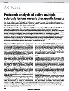
‘ECDFAu@““(S) is a1 inear ECDF that has the same average and the same average deviation as the actual distribution of S. We calculate its slope and origin (also in linear time) from the following set of equations (see figure 2): Y (2) = Slope, . x + Origin, Y (Average, + 2 AverageAbsoluteDeviation,) = 1 Y(Average, - 2 AverageAbsoluteDeviation,) = 0

(4 . 2)

4. Practical Considerations

18

slope, =

n

1

4 AvgAbsDev, = 4 ~~cl Iaverage, -

1 2

origin, = - - slope, average,

VtdUeil

(4 . 3)

where valueI,..., are the values of the keys of the set S. The approximation Y(x) is then scaled so that instead of returning values from 0 to 1, it will return integers between 1 and r(n): H,(x) = 1 r(n)(x.slope, + origin,) + 1 J

(4 . 4)

and then it is embedded in a conditional (see figure 2) to insure that it returns only valid bin indices, even for atypical values of x. When the distribution has a very steep slope, the average deviation tends to zero,_ but we will see next that this problem can be solved easily.

r(n)

1 Average, I Av~v. 4 . AverageAb&luteDeviation,

Figure 2.: The hashing function.

Note that many other possible hashing functions satisfying the requisites of the algorithm can be used [17,2]. We chose a piece-wise linear one because of its simplicity, and we will use it for all distributions because the potential advantages of more precise approximations do not seem to justify the increase in calculation complexity. These approximations give us the hashing functions that we need so as to partition each of the sets which is generated throughout the recursion (for each set that we partition, we compute a new set of statistical parameters).

ia

4.2 Graceful Degradation when 3c is not Satiafied

4.2 Graceful Degradation when

3C

is not Satisfied

Here we analyze what happens when there is absolutely no requirement on the order or distribution of the data to be sorted. In the description of Adaptsort we see that after calculating the statistical parameters of a sequence so as to build the hashing function, we check for the slope of the distribution. If this slope is excessive, the algorithm chooses smallsort for the part of the tree below this sequence. A key question is: what is an excessive slope? For the analysis of the asymptotic behavior of the algorithm, 3C is an adequate criterion, and any constant will do, but for practical applications we can choose an optimal value for the maximum slope that will result in a better performance. To obtain this, we equate the time it would take Quicksort to sort a sequence and the time it would take Adaptsort to do it

(4 . 5)

which results in

Q m a x

-

=

9

k n K k 72 - jp(Ig 0 2 [ kno

)I

n l g n -2 =-no [ lgn, I

(4 . 6)

In practice, we can use this optimal criterion to decide when to sort a sequence as if it didn’t satisfy 3C, even though it may actually satisfy it, or to use Adaptsort even though the data may not satisfy the global 3C, because it is being sorted locally faster than it would with the fallback sort. The reason for this is that although Adaptsort would be asymptotically better, we can do better by switching to an O(nIgn) sort (by definition of amal) for the finite size sub-sequence we are sorting, when the slope exceeds CY~,,. The function MaxSlope that appears in the Pidgin Algol description of the algorithm corresponds to this calculation. . If 3C were not satisfied, Adaptsort simply changes strategies for the part of the data that caused the problem, and since the statistics take only O(n) time, it will run at worst in O(n lgn) time if this happens almost everywhere. Hence, even though 3C may not be satisfied, there is a graceful performance loss, and in practical terms this loss might be negligible for most sets that are usually sorted (i.e., neither lengths of segments of Brownian movement [13], nor atomic decay times, nor unbounded salaries, etc.)

20

5. Space Complexity of Adaptsort

$5 Space Complexity of Adaptsort Looking at the Pidgin Algol description of the algorithm, we notice that the “Foreach . . . ” loop produces elements which are consumed by “Put In Bin”, freeing and occupying respectively one cell of storage. Therefore, the elements to be sorted, in fact, are never moved; only pointers are reset to point to other locations. A list representation is necessary to perform all the required operations within the given time constraints, so just for the set we need space for n values and n pointers. The space required for the recursion is used basically in local arrays of pointers (see Section 2) that point to the partially formed sublists, so that appending elements to any of these sublists can be done in constant time. The size of the biggest array is m. From then on the size of the arrays used in deeper levels of recursion decreases very fast. The size of the arrays used at recursion level d (starting the count with 1 for the top level) will be of O(n[(1i2)d]. Th e algorithm expands through the recursion an implicit tree of arrays in a depth first fashion. Since the arrays are no longer needed when the algorithm pops a level up in the recursion (see Section 2), this space can The arrays are no longer needed once we pop a level in the recursion because be reused. they are used only to keep pointers to the list of subsequences while we partition and sort the . subsequences. But, when we pop a level of recursion we have just completed the joining of the sorted subsequences, so the array is no longer needed. Since no more than 1 array is needed for each unfinished recursion level, it is clear that the total space requirements for the arrays isofO(fi)( we h ave a series which decreases faster than a geometric series, and whose initial term is fi). In any Algolic language the reuse of the space we used in the local arrays comes for free, while in others it may come at the expense of garbage collection. If for some reason the arrays’ space were not reused (either explicitly or through the space allocation management), - their number would grow very fast as we go deeper in the recursion and a simple calculation shows that at recursion level d, we would need n* array locations. To avoid unnecessary calculations, we can get an O(nlg lg n) space upper bound directly from the time performance of the algorithm. Nonetheless, for any reasonable value for n, the space lost even if we do not reuse the arrays, is minimal (e.g., to sort a million elements, the top level needs one array of a thousand locations, the second level will have a thousand arrays of an average size of 32. At this level the sets hanging from the arrays are smaller than the threshold which makes it faster to switch into Quicksort, so the recursion of Adaptsort ends having used about 3.3% of n for arrays space). Hence, from the practical point of view even if we do not reuse the arrays space, the necessary storage increases very little. In conclusion, Adaptsort has an O(n) space complexity, and if the data is already in a list, the extra space- requirement is only O(fi), and we can consider the algorithm as to be working basically “in place”.

6. Parallel AdaptSort

I

Zl

$6 Parallel AdaptSort For each sequence at any recursion level, first the set has to be completely partitioned. As soon as that is done all its subsequences can be sorted concurrently. Since the optimal number of partitions is fairly big, as soon as the original set is partitioned once, there are enough tasks to keep many processors busy most of the time in a natural way. Since the set is sorted in place, and multiple processors can be doing some sorting tasks, it seems as if there is a risk of creating havoc with the list unless a quite restrictive control to the list access is established. This is not so because each process works on a piece of the list disjoint from all others. Once a process is granted access to a pointer to a list, it can go ahead and need not worry about concurrent tasks being performed simultaneously with other parts of the same list. So in principle, the bottleneck would be in the access to the memory. Both the calculation of statistical parameters and the partitioning of each sequence are ideal tasks to be done faster with a pipelined floating point processor. Since these sequences are always relatively big, and additions and multiplications are needed for each element, the pipeline of such a processor would be used efficiently, with the consequent speed-up. Another way of increasing the speed would be to modify the hardware by adding a sorting net [lo]. T his net could sort the small sets for which Adaptsort now uses Quicksort. Since this net could function in a pipelined mode, the basic task of the program would be only to partition recursively the sets, send them one after the other to the net to get them sorted, and then concatenate the sorted sublists.

7. Matrix Sort

22

$7 Matrix Sort We have seen that a partition/concatenate sort can work in time less than O(nlgn) . Hence, it is natural to ask: can we do the same with a split/merge sorting scheme? (i.e., analogously to the relation between Quicksort and Mergesort) Well, it seems we cannot. The data structure for such a Mergesort, using square root as the partitioning function is interesting in the sense that if the set to be sorted is loaded in contiguous locations of memory, these can be looked as forming a square array which is partitioned into its columns. Recursive calls for each of the columns will sort these columns, and then the columns will be merged to obtain the sort of the full set. Since each column also will be stored in a block of contiguous locations, we can consider each column recursively as a new square submatrix, whose columns will again be considered in such a way, until we reach a column of less than a certain size. At this point, exactly as in Quicksort, we can switch to any simple in-place sorting algorithm. Note that in the deeper levels of recursion, there is no extra arithmetic for sub-subindices, but just added offsets. That is, the program should deal explicitly with the calculation of the location of the elements of the arrays of deeper levels of recursion. For the sake of simplicity the size of the set will be assumed to be ni2q) with both n, and Q positive integers, so that we can recursively keep subdividing the matrix into square submatrices until the column size drops to no. (At the q-th recursion level) We will see that the difficulty with this algorithm lies in the multiple source merging, which limits its running time to O(nlgn) . To merge these columns we can maintain a priority queue which will have pointers to the partially consumed (by the merge) columns. At each step of the merge, the element pointed to by the top of the priority queue is taken out from its column and appended to the current merge buffer. The queue has to be updated each time the smallest - element is taken from the queue, by introducing the next element of the same column into its appropriate position in the queue. This can be implemented as a heap with as many elements as columns are being merged, so it would take an expected time of O(lg (number of columns)) to pick an element from one of the columns being merged. Since the number of columns for a square matrix with n elements is @, we get the following recurrence:

T(no) = Kp, l&b) = Kt T(n) = fiT(lh) + qJnk(lhq

(7 . 1)

In this recurrence, we no longer have a linear independent term, as in adaptive sort. KP stands for the time it takes to pick a column from the priority queue, put its next element in the merged buffer, and update the queue.

23 *

7. Matrix Sort T(4) = n,T(n,) + K,nz I&,) WC)

= niT(ni) + K,nb lg(nf)

(7 . 2)

= K,nt + K,nft lg(n,)[l + 21 T(4) = Ktnl, + K,nt lg(n,)[l + 2 + 41

From the preceding expressions, it is clear that the general term is: ) TbOWV) = &q=‘

+ Kpni2*) lg(n,) me 2’ ;= 0

Kt = 7pY n, + Kp lg(no)(2m - 1) 0 [

1

(7 . 3)

By renaming variables as in the previous recurrence: T(n) = n = n Kt- + K,(kn - 43no) I no

=

1

(7 . 4)

n [K, k no + K&g n - lg no)]

= n w* -Kp)kno + K&n]

-

This last equation can be easily verified by induction, and it shows that matrix sort has an expected time complexity O(n lg n) . In the worst case each of the m lists has a single element, so that merging them in linear time would be equivalent to sorting by comparisons in linear time, which is not possible [IO]. So it seems that there is no Mergesort that takes time of only O(n lg Ign) . Otherwise, matrix sort has the advantage of not needing to make statistical measures, and does not need to put the keys in a list. It needs about 2n locations of storage, because of the buffers needed to make the merging. The biggest one is needed to merge the n elements contained in the fi columns of the top level.

8. Experimental resulta

4

.

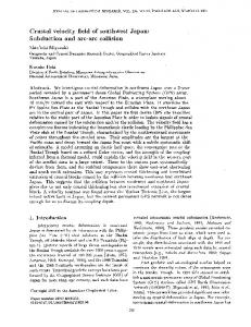
$8 Experimental results The program was tested on a DEC-20/60 and on a Foonly F2 machine (a KA-10 emulator) The numerical values given in this section correspond to both programs coded in InterLisp (without interspersing machine language). The data samples were lists of uniformly distributed random numbers. Since the speed of this algorithm depends heavily on the speed of floating point operations, as well as on its coding and compilation, the following results are just suggestive but not conclusive. Furthermore, as has been shown in [14,15] for Quicksort, variations of the algorithm, as well as the way inner loops are compiled could improve the performance of Adaptsort substantially. The crossover point between Quicksort and Adaptsort was found in sets of 150 elements. For sets of 20,000 elements Quicksort took 48% more time than Adaptsort. The following graph shows a comparison of the average times required for sets of different sizes. Time

1.0

0.5

0.0 -

150

10000

20000

Size

Figure 3.: w on a KL-10 From the values of this experiment, we can calculate the values of K, and Kq for Adaptsort and Quicksort respectively. Replacing these values in the respective expressions for T(n), we get that the constant. terms in TAdaptsort(n~ g et approximately canceled, so that we get the following (approximate) comparative equations for the two methods (for the Foonly): TAduptsort(n) = 205 n lg Ig n psec. Tguicksort(n) = 77 n lg n psec.

(8 . 1)

Further experimentation as well as fine tuning of the algorithm would provide more conclusive answers.

9. An Implementation of Adaptsort

25

$9 An Implementation of Adaptsort The algorithm was implemented in InterLisp because of the flexibility it provides, and is not intended to be particularly fast. A Pascal version was written first, but it looked quite obscure compared to this Clisp version, and is certainly longer. (Clisp looks more like Algol than Lisp, but may be difficult to follow if you are completely unfamiliar with Lisp) The following is very similar to the version of Adaptsort which was implemented, but all unnecesary details, declarations and obvious functions are not included. Nonetheless, this is not intended as a description of the algorithm, for which the reader should see section 2. As regards to notation, let is a lambda binding (binds a list of identifiers to a list of values which follow the be), z-1 is equivalent to (cur z) and z::l is equivalent to (cdr 2). Keywords are set in bold font.

(*Ad.sortirthocoreofthesort, rndi~relativel~slrailarto) (reeSoction1))

(*thePidgIn-Algoldorcriptionofthoalgorithln. (AdSort [lambda (S Size)

(* S ir a parameter; Sizealocaltarlable)

Size + (length S) (if Size is l mailer than Threshold then (Quicksort S)

(* F8rteriorrmallerrotr)

elee (let Npartit Rack be (fix (rqrt Size)) nil do (*Rack andNpartitarelocalvariabler) (AdStats S)

(* Calculateparameterr of dirtribution)

(if Slope > MaxSlope then (Quicksort S)

(* Couldn't break down this rubretroll) *

else Rack *- (array Npartit)

(*Back holds pointerrto partitlonr)

[repeatwhile S do (X t S) (*Nor, partitiontheretS) (S 4-- S::l) (Insert X Rack (AdSlot] (AdJoinsorts 1)

(* uortallpartitione andconcatenatethem)

(* Eetimateetheparameterr of a linear approxfmatlontothe) (* dietributfonof thevalues of thekeye. Itrorksaea) (* eideeffectbyoettingtheglobalvaluesSLOPEandOBIGIN) (AdStats [lambda (S) (setn Avg (for Value in S sum Value) / Size) [setn SurnDev (for Value in S aum (abs Avg-Value] [setn Slope (if (TooSmall SumDev) then oo else Size / (4 * SumDev] (eetn Origin 0.5 - Slope * Avg])

9. An Implementation of Adaptsort

26

.

(* AdSlot, rhichisthehaehingfunctlonHe(n) userthevrluer (* slope, origin andXto choooea rlot(bin) fntherack) (AdSlot [lambda(nil) [eetn Slot 1 + Npartit * ( Origin + Slope * X:1] (if (Slot is less than 1) then 1 elee( if Slot ie greater than Npartit then Npartit else Slot)])

(* CallrecursivelyAD.sortto sort each liethangingfromtherrck,

(*then join rlll%etr oneafkrtheothertoreturntheeorted

and)

requence)

(AdJoinsorts [lambda nil (for i from 1 to Npartit do (seta Rack i (AdSort (elt Rack i) ‘nobind))) (eetn FirstIndex 1) (while (elt Rack FirstIndex) = nil do (setn FirstIndex FintIndex+l)) LastNonEmpty - (last (elt Rack FirstIndex))

[for i from FirstIndex+l to Npartit do

(* gothroughtherrck joining sublirtr)

(CurrList + (elf Rack i)) (if CurrList

(* 601~ slots oftherackmaybe emptp(nil))

then (frplacd LastNonEmpty CurrList) LastNonEmpty a

- (last CurrList)

else nil] (elt Rack FirstIndex])

(* return apolnter totheconcatenrtion)

10. Concluding Remarks

e-m

-

27

5 10 Concluding F?,emarks We have presented an algorithm that has an asymptotic O(n lglgn) worst-case time complexity for sets of bounded length keys with bounded repetitions (such sets satisfy our fractalness criterion). We have also seen that from a practical point of view, we may sort conveniently sets that do not satisfy TC , and that even for such sets, the degradation of performance may be small in practice. and furthermore cannot be worse than O(n Ign) for any distribution. The algorithm is fast, is simple to code and is particularly well suited both for parallel processing and for external sorting. For data which is already in a list it works basically “in . place”. I would like to draw the attention of the reader to several problems which were left unsolved: (a) The calculation of cy,,, (the slope below which Adaptsort is faster than Quicksort) was done taking no (the sequence size beyond which Adaptsort is faster than Quicksort), as a constant and n, was defined as a constant based on a the selection of the partitioning function +d = n112. This was useful to establish bounds and asymptotic estimates, but to improve the practical performance of the algorithm, it would be worthwhile to consider them as coupled, and find their optimal values.

-

(b) We have mentioned that there is a continuum of algorithms in between Quicksort and Distributive Sorts, which results from the values of p and q that we chose for determining the number of sets into which we partition each set of size n according with r(n) = pn? This continuum is reflected in the properties of interest of the algorithms. Namely, Adaptsort (P = 1, !I = l/2) has both a time complexity and a distribution sensitivity that are between Quicksort (p = 2, q = 0) and Distributive Sorts (p = l/k, q = 1). Optimality conditions under diverse criterions could be developed. (c) We used a partitioning scheme (ECDFMinM”= ) that has a provably good asymptotic behavior, but replaced it with a more robust one (ECDFAugD”“) for practical applications. Proofs of its asymptotic behavior would be interesting. (d) We introduced a “badness” measure for distributions (7C ), we used it profitably for the asymptotic analysis, and we showed that this is a sufficient, but not necessary condition. We discussed a tight condition, that happens to be recursive. It would be interesting to provide non-recursive conditions tighter than jtC . (e) We briefly described how Adaptsort can be implemented in a parallel machine, but we did not analyze this further. It would be interesting to develop realistic models of its behavior (we assumed a global shared memory, for which contention must be dealt with; another alternative could be local memories, in which case the necessary information transfers

28

10. Concluding Remarks

must be taken into account) and to experiment with implementations. (f) Our experimental version could certainly be improved and more comparative tests run on real data so as to obtain more conclusive evidence as regards to the practicality of Adaptsort.

12. References

2Q

5 11 Acknowledgements I want to thank the help I received from numerous people. I discussed it initially with Cordell Green. Jorge Phillips criticized early drafts of this paper. Ignacio Zabala, Glenn Galfond, Peter Eichenberger and Ken Clarkson were most helpful in pointing out weak points. Donald Knuth and David Shaw referred me to related literature. Harry Mairson made useful comments refering to matrix sort. I appreciate the encouragement I received from Robert Tarjan and from Robert Mathews. Of course, all the faults that may remain are mine.

$12 References

-

PI

Aho, Hopcroft & Ullman: The Design and Analysis of Computer Algorithms, (1974) Addison- Wesley.

PI

Dobosiewicz, W.: Sorting by Distributive Partitioning, Information Processing Letters, vol 7, n.1 (1978) ~1-6.

PI

Feller, D.: An Introduction to Probability Theory and its Applications (1950), Vol.1, John Wiley & Sons Inc.

PI

Frazer, W. and McKellar A., Samplesort: A Sampling Approach to Minimal Storage Tree Sorting, Journal of the ACM, vol 17, n.3 (1970) p496-507.

PI

Green, C. and Barstow, D.: On Program Synthesis Knowledge, Artificial Intelligence, vol 10 (1978) p241-279.

PI

Hille, E. and Tamarkin, J.: Remarks on a Known Example of a Monotone Continuous Function, American Mathematical Monthly, Vol 36, ~255-264, Princeton University and Brown University.

-171 PI PI

Hoare, C.:’ Quicksort, Computer Journal 5:l lo-15 (1962). Hoel, Port & Stone: Introduction to Probability Theory, (1971) Houghton Mifflin Co. Karp, R.: Exercise 38 in Section 5.2.1. of The Art of Computer Programming, Vol 3 by D. Knuth.

PO1

Knuth, D.: The Art of Computer Programming, Vo1.3, Sorting and Searching, (1973) Addison- Wesley.

WI

Lindstrom, E. and Vitter, J.: The Design and Analysis of BucketSort for Bubble Memory Secondary Storage, Technical Report No. CS-83-23 (1983), Department of Computer Science, Brown University.

12. References

30

I121

MacLaren, D.: Internal Sorting by Radix Plus Sifting, Journal of ACM 13 (1966) p404411.

WI

Mandelbrot, B: The Fractal Ceometry of Nature (1977), W. H. Freeman and Co.

WI

Sedgewick, R.: The Analysis of Quicksort Algorithms, Acta Informatica (1977), vol W )l

1151

Sedgewick, R.: Quicksort, STAN-CS-75-492, PhD Thesis (1975), Department of Computer Science, Stanford University.

P61

Shannon, C. and Weaver W.: The Mathematical Theory of Communication (1949), University of Illinois Press.

WI

Weide, B.: Statistical Methods in Algorithm Design and Analysis, CMU-CS-78-142, PhD Thesis (1978), Department of Computer Science, Carnegie Mellon University.