Sound Classification. Juan Pablo Bello. EL9173 Selected Topics in Signal
Processing: Audio Content Analysis. NYU Poly ...
Sound Classification Juan Pablo Bello EL9173 Selected Topics in Signal Processing: Audio Content Analysis NYU Poly
Classification • It is the process by which we automatically assign an individual item to one of a number of categories or classes, based on its characteristics. • In our case: • (1) the items are audio signals (e.g. sounds, tracks, excerpts); • (2) their characteristics are the features we extract from them (MFCC, chroma, centroid); • (3) the classes (e.g. speakers, instruments, phones, sound environment) fit the problem definition • The complexity lies in finding an appropriate relationship between features and classes
Example • 200 sounds of 2 different kinds (red and blue); 2 features extracted per sound
Example • The 200 items in the 2-D feature space
Example • Boundary that optimizes performance -> risk of overfitting (excessive complexity, poor predictive power)
Example • Generalization -> Able to correctly classify novel input
Classification of audio signals • A number of relevant tasks: • Source Identification • Automatic Speech Recognition • Automatic Music Transcription • Labeling/Classification/Tagging • Music/Speech/Environmental Sound Segmentation • Sentiment/Emotion Recognition
• Common machine learning techniques applied in related fields (e.g. image, natural language processing)
An audio classifier • Feature extraction: (1) feature computation; (2) summarization • Pre-processing: (1) normalization; (2) feature selection
Feature vector 1
• Classification: (1) use sample data to estimate boundaries, distributions or classmembership; (2) classify new data based on these estimations
Feature vector 2
Classification
Model
Feature set (recap) • Feature extraction is necessary as audio signals carry too much redundant and/or irrelevant information • They can be estimated on a frame by frame basis or within segments, sounds or tracks. • Many possible features: spectral, temporal, pitch-based, etc. • A good feature set is a must for classification • What should we look for in a feature set?
Feature set (what to look for?) • A few issues of feature design/choice: • Can be robustly estimated from available audio (e.g. spectral envelope vs onset rise times in polyphonies) • Relevant to classification task (e.g. MFCC vs chroma for source ID) -> noisy features make classification more difficult! • Feature set should be as invariant as possible to changes within the natural class’ range
Feature set (what to look for?) • We expect variability within sound classes • For example: trumpet sounds change considerably between, e.g. different loudness levels, pitches, instruments, playing style or recording conditions
• Classes are never fully described by a point in the feature space but by the distribution of a sample population
Features and training • Class models must be learned on many sounds to properly account for between/within class variations • The natural range of features must be well represented on the sample population
• Failure to do so leads to overfitting: training data only covers a sub-region of its natural range and class models are inadequate for new data.
Feature set (what to look for?) • Low(er) dimensional feature space -> Classification becomes more difficult as the dimensionality of the feature space increases.
• As free from redundancies (strongly correlated features) as possible • Discriminative power: good features result in separation between classes and grouping within classes
Feature distribution • Remember the histograms of our example. They describe the behavior of features across our sample population.
• It is desirable to parameterize this behavior
Feature distribution • A Normal or Gaussian distribution is a bell-shaped probability density function defined by two parameters, its mean (μ) and variance (σ2):
1 p e 2⇡
N (xl ; µ, ) =
(xl µ)2 2 2
L X 1 µ= xl L l=1
2
L X 1 = (xl L l=1
µ)2
Feature distribution • In D-dimensions, the distribution becomes an ellipsoid defined by a Ddimensional mean vector and a DxD covariance matrix:
L X 1 C(x, y) = (xl L l=1
µx )(yl
µy )
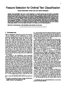
Feature distribution • Cx is a square symmetric DxD matrix: diagonal components are the feature variances; off-diagonal terms are their co-variances
*from Shlens, 2009
• High covariance between features shows as a narrow ellipsoid (high redundancy)
Data normalization • To avoid bias towards features with wider range, we can normalize all to have zero mean and unit variance:
x ˆ = (x
µ)/
µ=0
€
σ =1
€
PCA • Complementarily we can minimize redundancies by applying Principal Component Analysis (PCA) • Let us assume that there is a linear transformation A, such that:
2
a1 · x1 6 .. 4 .
aD · x 1
··· .. . ···
Y = AX 2 3 3 a1 a1 · xL 6 a2 7 ⇥ .. 7 = 6 7 x .. 7 1 . 5 6 4 . 5 aD · xL aD
x2
···
xL
⇤
• Where xl are the D-dimensional feature vectors (after mean removal) such that: Cx = XXT/L
PCA • What do we want from Y: • Decorrelated: All off-diagonal elements of Cy should be zero • Rank-ordered: according to variance • Unit variance • A -> orthonormal matrix; rows = principal components of X
PCA • How to choose A?
1 1 T Cy = Y Y = (AX)(AX)T = A L L
✓
1 XX T L
◆
AT = ACx AT
• Any symmetric matrix (such as Cx) is diagonalized by an orthogonal matrix E of its eigenvectors • For a linear transformation Z, an eigenvector ei is any non-zero vector that satisfies: Zei = i ei • Where λi is a scalar known as the eigenvalue • PCA chooses A = ET, a matrix where each row is an eigenvector of Cx
PCA • In MATLAB:
From http://www.snl.salk.edu/~shlens/pub/notes/pca.pdf
Dimensionality reduction • Furthermore, PCA can be used to reduce the number of features: • Since A is ordered according to eigenvalue λi from high to low • We can then use an MxD subset of this reordered matrix for PCA, such that the result corresponds to an approximation using the M most relevant feature vectors • This is equivalent to projecting the data into the few directions that maximize variance • We do not need to choose between correlating (redundant) features, PCA chooses for us. • Can be used,e.g., to visualize high-dimensional spaces
Discrimination • Let us define:
Proportion of occurrences of class k in the sample
Sw =
K X
(Lk /L)Ck
k=1
Within-class scatter matrix Covariance matrix for class k
Sb =
K X
global mean
(Lk /L)(µk
k=1
Between-class scatter matrix
µ)(µk
µ)T
Mean of class k
Discrimination • Trace{U} is the sum of all diagonal elements of U, s.t.: • Trace{Sw} measures average variance of features across all classes • Trace{Sb} measures average distance between class means and global mean across all classes • The discriminative power of a feature set can be measured as:
trace{Sb } J0 = trace{Sw } • High when samples from a class are well clustered around their mean (small trace{Sw}), and/or when different classes are well separated (large trace{Sb}).
Feature selection • But how to select an optimal subset of M features from our D-dimensional space that maximizes class separability? • We can try all possible M-long feature combinations and select the one that maximizes J0 (or any other class separability measure) • In practice this is unfeasible as there are too many possible combinations • We need either a technique to scan through a subset of possible combinations, or a transformation that re-arranges features according to their discriminative properties
Feature selection • Sequential backward selection (SBS): 1. Start with F = D features. 2. For each combination of F-1 features (inc. chosen F) compute J0 3. Select the combination that maximizes J0 4. Repeat steps 2 and 3 until F = M • Good for eliminating bad features; nothing guarantees that the optimal (F-1)dimensional vector has to originate from the optimal F-dimensional one. • Nesting: once a feature has been discarded it cannot be reconsidered
Feature selection • Sequential forward selection (SFS): 1. Select the individual feature (F = 1) that maximizes J0 2. Create all combinations of F+1 features including the previous winner and compute J0 3. Select the combination that maximizes J0 4. Repeat steps 2 and 3 until F = M • Nesting: once a feature has been selected it cannot be discarded
LDA • An alternative way to select features with high discriminative power is to use linear discriminant analysis (LDA) • LDA is similar to PCA, but the eigenanalysis is performed on the matrix Sw-1Sb instead of Cx • Like in PCA, the transformation matrix A is re-ordered according to the eigenvalues λi from high to low • Then we can use only the top M rows of A, where M < rank of Sw-1Sb • LDA projects the data into a few directions maximizing class separability
Classification • We have: • A taxonomy of classes • A representative sample of the signals to be classified • An optimal set of features • Goals: • Learn class models from the data • Classify new instances using these models • Strategies: • Supervised: models learned by example • Unsupervised: models are uncovered from unlabeled data
Instance-based learning • Simple classification can be performed by measuring the distance between instances. • Nearest-neighbor classification: • Measures distance between new sample and all samples in the training set • Selects the class of the closest training sample • k-nearest neighbors (k-NN) classifier: • Measures distance between new sample and all samples in the training set • Identifies the k nearest neighbors • Selects the class that was more often picked.
Instance-based learning • In both these cases, training is reduced to storing the labeled training instances for comparison • Known as “lazy” or “memory-based” learning. • All computations are performed during classification • Complexity increases with number of training instances. • Alternatively, we can store only a few class prototypes/models (e.g. class centroids)
Instance-based learning • We need to choose k to avoid overfitting, e.g., k = √L where L is the number of training samples
• Works well for well-separated classes; and an appropriate combination of distance metric and feature pre-processing
Instance-based learning • The effect of standardization (from Peltonen’s MSc thesis, 2001)
Instance-based learning • Mahalanobis distance: considers q the underlying distribution
d(x, y) =
(x
y)T C
1 (x
y)
Probability • Let us assume that the observations X and classes Y are random variables
*From Bishop’s Machine Learning book, 2007
Probability L = total number of blue dots ci = number of dots in column i rj = number of dots in row j nij = number of dots in cell ij Joint Probability Marginal Probability Conditional Probability
n
P (X, Y ) = P (Y, X) = Lij P ci P (X) = L = j P (X, Y ) P (Y |X) =
P (X, Y ) =
Symmetry rule Sum rule
nij ci
nij L
=
nij ci ci L
= P (Y |X)P (X) Product rule
Probability • Thus we can derive Bayes’ theorem as:
Posterior: probability of class i given an observation x
Likelihood: Probability of observation x, given class i
P (x|classi )P (classi ) P (classi |x) = P (x)
Prior: Probability of class i
Marginal Likelihood: Normalizing constant (same for all classes) that ensures posterior adds to 1
P (x) =
X i
P (x|classi )P (classi )
Probabilistic Classifiers • Classification: finding the class with the highest probability given the observation x • Find i that maximizes the posterior probability P(classi|x) -> Maximum A Posteriori (MAP) • Since P(x) is the same for all classes, this is equivalent to:
argmax[P (x|classi )P (classi )] i
• From the training data we can learn the likelihood P(x|classi) and the prior P(classi)
Gaussian Mixture Model • We can model (parameterize) the likelihood using a Gaussian Mixture Model (GMM) -> the weighted sum of K multidimensional Gaussian distributions:
P (x|classi ) =
K X
k=1
wik N (x; µik , Cik )
• Where wik are the mixing weights and:
1 N (x; µ, Cx ) = e D/2 1/2 (2⇡) |Cx |
1 2 (x
µ)T Cx
1
(x µ)
Gaussian Mixture Model • 1-D GMM (Heittola, 2004)
• With a sufficiently large K a GMM can approximate any distribution • However, increasing K increases the complexity of the model and compromises its ability to generalize
Gaussian Mixture Model • The model is parametric, consisting of K weights, mean vectors and covariance matrices for every class. • If features are decorrelated, then we can use diagonal covariance matrices, thus considerably reducing the number of parameters to be estimated (common approximation) • Parameters can be estimated using the Expectation-Maximization (EM) algorithm (Dempster et al, 1977). • EM is an iterative algorithm whose objective is to find the set of parameters that maximizes the likelihood.
K-means • Dataset: L observations of a D-dimensional variable x • Goal: find the partition into K clusters, each represented by a prototype μk, that minimizes the distortion:
J=
L X K X
l=1 k=1
rlk kxl
µk k22
• where the “responsibility” function rlk = 1 if the lth observation is assigned to cluster k, 0 otherwise • We don’t know the optimal rlk and μk
K-means 1. Choose initial values for μk 2. E (expectation)-step: keeping μk fixed, minimize J with respect to rlk
rlk =
⇢
1 0
if k = argmink kxl otherwise
µk k22
3. M (maximization)-step: keeping rlk fixed, minimize J with respect to μk
P rlk xl l µk = P l rlk
4. repeat 2 and 3 until J or the parameters stop changing
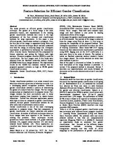
K-means
random centers
select k
recalculate centers
repeat
assign to cluster
end
*from http://www.autonlab.org/tutorials/kmeans11.pdf
K-means • Many possible improvements (see, e.g. Dan Pelleg and Andrew Moore’s work) • does not always converge to the optimal solution -> run k-means multiple times with different random initializations • sensitive to initial centers -> start with random datapoint as center; next center is farthest datapoint from closest center • sensitive to choice of K -> find the K that minimizes the Schwarz criterion (see Moore’s tutorial): L X l
(k)
kxl
µk k22 + (DK)logL
EM Algorithm • GMM: each cluster corresponds to a weighted Gaussian • Soft responsibility function: conditional probability of belonging to Gaussian k given observation xl lk
wk N (xl ; µk , Ck )
= PK
j=1
wj N (xl ; µj , Cj )
• Goal: find the parameters that maximize
log{p(X|µ, C, w)} =
L X l=1
log
(
K X
k=1
wk N (xl ; µk , Ck )
)
EM Algorithm 1. Initialize μk, Ck and wk 2. E-step: evaluate responsibilities ϒlk using current parameters 3. M-step: re-estimate parameters using current responsibilities
µnew k
P = Pl
Cnew = k
P
l
lk xl l
lk lk (xl
wknew
=
µnew )(xl k P l
P
l
lk
L
T µnew ) k
lk
4. repeat 2 and 3 until the log likelihood or the parameters stop changing
EM Algorithm
*From Bishop’s Machine Learning book, 2007
EM Algorithm • EM is both more expensive and slower to converge than K-means • Common trick: run K-means to initialize EM • Find cluster centers (means) • Compute sample covariances of the found clusters • Mixing weights -> fraction of L assigned to each cluster
MAP Classification • After learning the likelihood and the prior during training, we can classify new instances based on MAP classification:
argmax[P (x|classi )P (classi )] i
References • This lecture borrows heavily from Emmanuel Vincent’s lecture notes on instrument classification (QMUL - Music Analysis and Synthesis) and from Anssi Klapuri’s lecture notes on Audio Signal Classification (ISMIR 2004 Graduate School: http:// ismir2004.ismir.net/graduate.html) • Bishop, C.M. Pattern Recognition and Machine Learning. Springer (2007) • Duda, R.O., Hart, P.E. and Stork, D.G. Pattern Classification (2nd Ed). John Wiley & Sons (2000) • Witten, I. and Frank, E. Data Mining: Practical Machine Learning Tools and Techniques. Morgan Kaufmann (2005) • Shlens, J. A Tutorial on Principal Component Analysis, Version 3.01 (2009): http:// www.snl.salk.edu/~shlens/pca.pdf • Moore, A. Statistical Data Mining Tutorials: http://www.autonlab.org/tutorials/