Sound modeling: signal-based approaches

Chapter 2

Sound modeling: signal-based approaches Giovanni De Poli and Federico Avanzini c 2005-2009 Giovanni De Poli and Federico Avanzini Copyright ° except for paragraphs labeled as adapted from This book is licensed under the CreativeCommons Attribution-NonCommercial-ShareAlike 3.0 license. To view a copy of this license, visit http://creativecommons.org/licenses/by-nc-sa/3.0/, or send a letter to Creative Commons, 171 2nd Street, Suite 300, San Francisco, California, 94105, USA.

2.1 Introduction The sound produced by acoustic musical instruments is caused by the physical vibration of a certain resonating structure. This vibration can be described by signals that correspond to the time-evolution of the acoustic pressure associated to it. The fact that the sound can be characterized by a set of signals suggests quite naturally that some computing equipment could be successfully employed for generating sounds, for either the imitation of acoustic instruments or the creation of new sounds with novel timbral properties. A wide variety of sound synthesis algorithms is currently available either commercially or in the literature. Each one of them exhibits some peculiar characteristics that could make it preferable to others, depending on goals and needs. Technological progress has made enormous steps forward in the past few years as far as the computational power that can be made available at low cost is concerned. At the same time, sound synthesis methods have become more and more computationally efficient and the user interface has become friendlier and friendlier. As a consequence, musicians can nowadays access a wide collection of synthesis techniques (all available at low cost in their full functionality), and concentrate on their timbral properties. Each sound synthesis algorithm can be thought of as a digital model for the sound itself. Though this observation may seem quite obvious, its meaning for sound synthesis is not so straightforward. As a matter of fact, modeling sounds is much more than just generating them, as a digital model can be used for representing and generating a whole class of sounds, depending on the choice of control parameters. The idea of associating a class of sounds to a digital sound model is in complete

2-2

Algorithms for Sound and Music Computing [v.October 30, 2009]

accordance with the way we tend to classify natural musical instruments according to their sound generation mechanism. For example, strings and woodwinds are normally seen as timbral classes of acoustic instruments characterized by their sound generation mechanism. It should be quite clear that the degree of compactness of a class of sounds is determined, on one hand, by the sensitivity of the digital model to parameter variations and, on the other hand, on the amount of control that is necessary for obtaining a certain desired sound. As an extreme example we may think of a situation in which a musician is required to generate sounds sample by sample, while the task of the computing equipment is just that of playing the samples. In this case the control signal is represented by the sound itself, therefore the class of sounds that can be produced is unlimited but the instrument is impossible for a musician to control and play. An opposite extremal situation is that in which the synthesis technique is actually the model of an acoustic musical instrument. In this case the class of sounds that can be produced is much more limited (it is characteristic of the mechanism that is being modeled by the algorithm), but the degree of difficulty involved in generating the control parameters is quite modest, as it corresponds to physical parameters that have an intuitive counterpart in the experience of the musician. An interesting conclusion that could be already drawn in the light of what stated above is that the compactness of the class of sounds associated to a sound synthesis algorithm is somehow in contrast with the “playability” of the algorithm itself. One should remember that the ”playability” is of crucial importance for the success of a specific sound synthesis algorithm as, in order for a sound synthesis algorithm to be suitable for musical purposes, the musician needs an intuitive and easy access to its control parameters during both the sound design process and the performance. Such requirements often represents the reason why a certain synthesis technique is preferred to others. Some considerations on control parameters are now in order. Varying the control parameters of a sound synthesis algorithm can serve several purposes, the first one of which is certainly that of exploring a sound space, i.e. producing all the different sounds that belong to the class characterized by the algorithm itself. This very traditional way of using control parameters would nowadays be largely insufficient by itself. As a matter of fact, with the progress in the computational devices that are currently being employed for musical purposes, the musician’s needs have turned more and more toward problems of timbral dynamics. For example, timbral differences between soft (dark) and loud (brilliant) tones are usually obtained through appropriate parameter control. Timbral expression parameters tend to operate at a note-level time-scale. As such, they can be suitably treated as signals characterized by a rather slow rate. Another reason for the importance of time-variations in the algorithm parameters is that the musician needs to control the musical expression while playing. For example, staccato, legato, vibrato etc. need to be obtained through parameter control. Such parameter variations operate at a phrase-level time-scale. Because of that, they can be suitably treated as sequences of symbols events characterized by a very slow rate. In conclusion, control parameters are signals characterized by their own time-scales. Controls signals for timbral dynamics are best described as discrete-time signals with a slow sampling rate, while controls for musical expression are best described by streams of asynchronous symbols events. As a consequence, the generation of control signals can once again be seen as a problem of signal synthesis. This book is licensed under the CreativeCommons Attribution-NonCommercial-ShareAlike 3.0 license, c °2005-2009 by the authors except for paragraphs labeled as adapted from

Chapter 2. Sound modeling: signal-based approaches

2-3

2.2 Time-segment based models 2.2.1 Wavetable synthesis 2.2.1.1 Definitions and applications Finding a mathematical model that faithfully imitates a real sound is an extremely difficult task. If an existing reference sound is available, however, it is always possible to reproduce it through recording. Such a method, though simple in its principle, is widely adopted by digital sampling instruments or samplers and is called wavetable synthesis or sampling.1 A samplers is a device which is able to store and play back a large quantity of recorded sounds: most typically these are musical, instrumental sounds, but they may also be non-musical, environmental sounds. In fact the most appealing quality of wavetable synthesis is the possibility of working with an unlimited variety of sounds. From the implementation viewpoint, computational simplicity is certainly an advantage of the technique, which contrasts with the need of huge memory capacities (as an example, a contemporary piano synthesizer based on sampling may require tens of Gigabytes to store the entire instrument). The table look-up mechanism is in essence identical to that already outlined for the wavetable oscillator in Chapter Fundamentals of digital audio processing. The recorded sound is stored in a table of length L, and the synthesized sound x[n] is the result of reading the table using a phase signal φ[n] with a certain length M : x[n] = tab{φ[n]}, φ : [0, M − 1] → [0, L − 1]. (2.1) Simple playback one sound of the stored repertoire is obtained using the signal φ[n] = n and with M = L. In this case all the original samples of the stored sound are played back at the original speed. Using different signals φ[n] will result in modifications of the original sound. However the possibilities of modification are rather limited, as it would be for the sound recorded by a tape deck. The most common modification is obtained by varying the speed when reproducing the sound, which results in a pitch transposition. Other simple transformations include time-reversal (i.e. table read out starting from the last sample), looping (i.e. periodically scanning the wavetable or part of it), cutting and possibly rearranging portions of the original sound. In particular, it is possible to adopt looping techniques with almost any stationary portion of sounds. One method of improving the expressive possibilities of samplers is store multiple instances of a single instrumental note for different dynamics (e.g. from soft to loud key velocities in the case of the piano), or even different pitches, and switching or interpolating between these upon synthesis. This approach is called multisampling. During synthesis, linear interpolation between stored sounds is performed as function of the desired dynamics. Historically, the use of samplers may be traced back to a time where digital sound was still to come and magnetic tapes had just made their appearance. So-called musique concr`ete, first developed in Paris in late 1940’s mainly through the work of french composer Pierre Schaeffer and colleagues, stemmed from an aesthetic practice that was centered upon the use of sound as a primary compositional resource. The development of this music was facilitated by the emergence of then new technologies such as microphones and magnetic tape recorders. Compositions were based on (usually non-musical) sounds acquired through a microphone, recorded on tape, manipulated and recombined in variety of ways, and finally played back from tape. 1

In musical jargon it has become customary to use the term sample to denote an entire sound, recorded and stored in a table. To avoid confusion, in this book we only use the term sample only with the meaning explained in Chapter Fundamentals of digital audio processing, i.e. a single value of a digital signal. This book is licensed under the CreativeCommons Attribution-NonCommercial-ShareAlike 3.0 license, c °2005-2009 by the authors except for paragraphs labeled as adapted from

2-4

Algorithms for Sound and Music Computing [v.October 30, 2009]

Nowadayes wavetable synthesis techniques are presented as a method for reproducing natural instrumental sounds that are comparable in quality with the original instruments. This is the main reason why the most popular commercial digital keyboards adopt this synthesis technique. Of course, sampling cannot feature all the expressive possibilities of the original instrument. 2.2.1.2 Tranformations: pitch shifting, looping Pitch shifting, i.e. transposition of the original pitch of the recorded sound, is the simplest transformation obtainable with wavetable synthesis. Assume that the original sample rate and the playback sample rate are the same. If we read the entire table (of length L) with a signal φ of length M , then the overall sound duration is compressed or expanded by a factor M/L and the pitch is transposed by a factor L/M . An overall transposition of a factor L/M can be obtained by reading the table with the signal ¹ º L φ[n] = n , n = 0, . . . , M − 1. (2.2) M As an example, if 3M = 2L the sound will be transposed upwards by a perfect fifth (i.e. by a ratio of 3/2). However, φ needs not to be a ramp that rises linearly in time. In the case where φ is still a monotonic signal, but changes its slope during time, the transposition will become time-dependent. Although the pitch shifting outlined above is simple and straightforward to implement, it has to be noted that substantial pitch variations are generally not very satisfactory as a temporal waveform compression or expansion results in unnatural timbral modifications, which is exactly what happens when the playing speed is changed in a tape recorder. Satisfactory quality and timbral similarity between the original tone and the transposed one can be obtained only if small pitch variations (e.g. a few semitones) are performed. As an example, sampling a piano with a reasonable quality along the entire instrumental extension requires that many notes are stored (e.g. three for each octave). In this way, notes that have not been sampled can be obtained from the available ones through transposition of max. two semitones. M-2.1 Import a .wav file of a single instrument tone. Scale it (compress and expand) to different extents and listen to the new sounds. Up to what scaling ratio are the results acceptable?

Often it is desired to vary the sound also in function of other parameters, the most important being the intensity. To this purpose it not sufficient to change the sound amplitude by a multiplication, by it is necessary to modify the timbre of the sound. In general louder sounds are characterized by a sharper attack and by a brighter spectrum. In this case a technique could be to use a unique sound prototype (e.g. a tone played fortissimo) and then obtaining the other intensity by simple spectral processing, as low pass filtering. A different and more effective solution, is to use a set of different sound prototype, recorder with different intensity (e.g. tones played fortissimo, mezzo forte, pianissimo) and then obtaining the other dynamic values by interpolations and further processing. This technique is thus characterized by high computational efficiency and high imitation quality, but by low flexibility for sounds not initially included in the repertoire or not easily obtainable with simple transformations. There is a trade-off of memory size with sound fidelity. In order to employ efficiently the memory, often the sustain part of the tone is not entirely stored but only a part (or few significant parts) and in the synthesis this part is repeated (looping). Naturally the repeated part should not be to short, to avoid a static character of the resulting sound. For example This book is licensed under the CreativeCommons Attribution-NonCommercial-ShareAlike 3.0 license, c °2005-2009 by the authors except for paragraphs labeled as adapted from

2-5

Chapter 2. Sound modeling: signal-based approaches

to lengthen the duration of a note, first the attack is reproduced without modification, then the sustain part is cyclically repeated, with possible cross interpolation among the different selected parts, and finally the sound release stored part is reproduced. Notice that if we want to avoid artefacts in cycling, particular care should be devoted to choosing the points of the beginning and ending of the loop. Normally an integer number of periods is used for looping starting with a null value, to avoid amplitude or phase discontinuities. In fact these discontinuities are very annoying. To this purpose it may be necessary to process the recorded samples by slightly changing the phases of the partials. M-2.2 Import a .wav file of a single instrument tone. Find the stationary (sustain) part, isolate a section, and perform the looping operation. Listen to the results, and listen to the artifacts when the looped section does not start/end at zero-crossings.

If we want a less static sustain, it is possible to individuate some different and significant sound segments, and during the synthesis interpolate (cross-fade) among subsequent segments. In this case the temporal evolution of the tone can be more faithfully reproduced.

2.2.2 Overlap-Add (OLA) methods The definition Overlap-Add (OLA) refers in general to a family of algorithms that produce a signal by properly assembling a number of signal segments. OLA methods are developed both in the time domain and in the frequency domain. Here we are interested in reviewing briefly time-domain approaches, while in Sec. 2.3 we will address time-frequency representations. 2.2.2.1 Basic time-domain overlap-add Given a sound signal x[n], a sequence of windowed segments xm [n] can be constructed as xm [n] = x[n]wa [n − mSa ],

(2.3)

where wa [n] is an analysis window and Sa is the analysis hop-size, i.e. the time-lag (in samples) between one analysis frame and the following one. If the window wa is N samples long, then the block size, i.e. the length of each frame xm [n], will be N . In order for the signal segments to actually overlap, the inequality Sa ≤ N must be verified. When Sa = N the segments are exactly juxtaposed with no overlap. Given the abovePsignal segmentation, time-domain overlap-add (OLA) methods construct an output signal y[n] = m ym [n], where the segments ym are modified versions of the input segments xm . As an examples, they can be obtained by modifying Sa in Eq. (2.3), or by repeating/removing some of the input segments xm . In the absence of modifications, this procedure reduces to an identity (y[n] ≡ x[n]) if the overlapped and added analysis windows wa sum to unity: X X X y[n] = xm [n] = x[n]wa [n − mSa ] = x[n] ⇔ Awa [n] , wa [n − mSa ] ≡ 1. (2.4) m

m

m

If this condition does not hold, then the function Awa acts on the reconstructed signal as a periodic amplitude modulation envelope, with period Sa . Depending on the application and on the window length N , this amplitude modulation can introduce audible artifacts. This kind of frame rate distortion can be seen in the frequency domain as a series of sidebands with spacing Fs /Sa in a spectrogram of the output signal. In fact, one may prove that the condition Awa ≡ 1 is equivalent to the condition This book is licensed under the CreativeCommons Attribution-NonCommercial-ShareAlike 3.0 license, c °2005-2009 by the authors except for paragraphs labeled as adapted from

2-6

Algorithms for Sound and Music Computing [v.October 30, 2009]

original signal

reconstructed signal

0

0.01

0.02

0.03

0.04

0.05

0.06

0.07

t (s)

Figure 2.1: An example of OLA signal reconstruction, with triangular windowing.

W (ejωk ) = 0 at all harmonics of the frame rate Fs /Sa . Figure 2.1 illustrates an example of signal reconstruction using a triangular window, which satisfy the condition of Eq. (2.4). A widely studied effect is time-stretching, i.e. contraction or expansion of the duration of an audio signal. Time-stretching algorithms useful in a number of applications: think about wavetable synthesis, post-synchonization of audio and video, speech technology at large, and so on. A timestretching algorithm should ideally shorten or lengthen a sound file composed of Ntot samples to a 0 = αN , where α is the stretching factor. Note that a mere resampling of the new desired length Ntot tot sound signal does not provide the desired result, since it has the side-effect of transposing the sound: in this context resampling is the digital equivalent of playing the tape at a different speed. What one really wants is a scaling of the perceived timing attributes without affecting the perceived frequency attributes. More precisely, we want the time-scaled version of the audio signal to be perceived as the same sequence of acoustic events as the original signal, only distributed on a compressed/expanded time pattern. As an example, a time-stretching algorithm applied to a speech signal should change the speaking rate without altering the pitch. Time-domain OLA techniques are one possible approach to time-stretching effects. The basic OLA algorithm described above can be adapted to this problem by defining an analysis hop size) Sa and a synthesis hop size Ss = αSa , scaled by the stretching factor, that will be applied to the output. An input signal x[n] is then segmented into frames xk [n], each taken every Sa samples. The output signal y[n] is produced by reassembling the same frames xk [n], each added to the preceding one every Ss samples. However this repositioning of the input segments with respect to each other destroys the original phase relationships, and constructs the output signal by interpolating between these misaligned segments. This cause pitch period discontinuities and distortions that can produce heavily audible artifacts in the output signal. 2.2.2.2 Syncronous overlap-add In order to avoid phase discontinuities at the boundaries between frames, a proper time alignment of the blocks has to be chosen. The synchronous overlap-add (SOLA) algorithm realizes such a proper This book is licensed under the CreativeCommons Attribution-NonCommercial-ShareAlike 3.0 license, c °2005-2009 by the authors except for paragraphs labeled as adapted from

2-7

Chapter 2. Sound modeling: signal-based approaches

Lk

Original signal mk

mk+1

Lk+1

(k+1)Ss kS s

x k+2[n]

x k+1[n]

y[n] x k [n] x k+1[n]

Sa Sa

x k+2[n]

Time−stretched signal

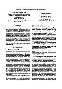
Figure 2.2: The generic SOLA algorithmic step.

alignement, and provides a good sound quality (at least for values of α not too far from 1) while remaining computationally simple, which makes it suitable even for real-time applications. Let N be the analysis block length. In the initialization phase the SOLA algorithm copies the first N samples from x1 [n] to the output y[n], to obtain a minimum set of samples to work on: y[j] = x1 [j] = x[j]

for j = 0 . . . N − 1.

(2.5)

Then, during the generic kth step the algorithm tries to find the optimal overlap between the last portion of the output signal y[n] and the incoming analysis frame xk+1 [n]. More precisely, xk+1 [n] is pasted to the output y[n] starting from sample kSs + mk , where mk is a small discrete time-lag that optimizes the alignement between y and xk (see Fig. 2.2). Note that mk can in general be positive or negative, although for clarity we have used a positive mk in Fig. 2.2. When the optimal time-lag mk is found, a linear crossfade is used within the overlap window, in order to obtain a gradual transition from the last portion of y to the first portion of xk . Then the last samples of xk are pasted into y. If we assume that the overlap window at the kth SOLA step is Lk samples long, then the algorithmic step computes the new frame of the input y as ½ (1 − v[j])y[kSs + j] + v[j]xk [j] for mk ≤ j ≤ Lk (2.6) y[kSs + j] = xk [j] for Lk + 1 ≤ j ≤ N where v[j] is a linear smoothing function that realizes the crossfade between the two segments. The effect of Eq. (2.6) is a local replication or suppression of waveform periods (depending on the value of α), that eventually results in an output signal y[n] with approximately the same spectral properties of the input x[n], and an altered temporal evolution. At least three techniques are commonly used in order to find the optimal value for the discrete time lag mk at each algorithmic step k: 1. Computation of the minimum vectorial inter-frame distance in an L1 sense (cross-AMDF) 2. Computation of the maximum cross-correlation rk (m) in a neighborhood of the sample kSs . Let M be the width of such neighborhood, and let yMk [i] = y[kSs + i] for i = 1 . . . M − 1, and xMk [i] = xk+1 [i] for i = 1 . . . M − 1. Then the cross-correlation rk (m) is computed as rk [m] ,

M −m−1 X

yMk [i] · xMk [i + m],

m = −M + 1, . . . , M − 1.

i=0

This book is licensed under the CreativeCommons Attribution-NonCommercial-ShareAlike 3.0 license, c °2005-2009 by the authors except for paragraphs labeled as adapted from

(2.7)

2-8

Algorithms for Sound and Music Computing [v.October 30, 2009]

Then mk is chosen to be the index of maximal cross-correlation: rk [mk ] = maxm rk [m]. 3. Computation of the maximum normalized cross-correlation, where every value taken from the cross-correlation signal is normalized by dividing it by the product of the frame energies. The latter technique is conceptually preferable, but the second one is often used for efficiency reasons. M-2.3 Write a function that realizes the time-stretching SOLA algorithm through segment cross-correlation.

M-2.3 Solution function y = sola_timestretch(x,N,Sa,alpha,L) %N: block length; Sa: analysis hop-size; alpha: stretch factor; L: overlap int. Ss = round(Sa*alpha); %synthesis hop-size if ( (Sa > N) || (Ss >= N) || Ss > N-L) error(’Wrong parameter values!’); end if (rem(L,2)˜= 0) L = L+1; end M = ceil(length(x)/Sa); x(M*Sa+N)=0; y(1:N,1) = x(1:N);

%number of frames %now x is exactly M*Sa samples %first frame of x is written into y;

for m=1:M-1 %loop over frames frame=x(m*Sa+1:N+m*Sa); %current analysis frame framecorr=xcorr(frame(1:L),y(m*Ss:m*Ss+(L-1))); [corrmax,imax]=max(framecorr); %find point of max xcorrelation fade = (m*Ss-(L-1)+imax-1):length(y); %points for crossfade fadein = (0:length(fade)-1)/length(fade); %from 0 to 1 fadeout = 1 - fadein; %from 1 to 0 y=[y(1:(fade(1)-1)); (y(fade).*fadeout’ +frame(1:length(fade)).*fadein’); ... frame(length(fade)+1:length(frame))]; end

2.2.2.3 Pitch synchronous overlap-add A variation of the SOLA algorithm for time stretching is the pitch synchronous overlap-add (PSOLA) algorithm, which is especially used for voice processing. PSOLA assumes that the input sound is pitched, and exploits the pitch information to correctly align the segments and avoid pitch discontinuities. The algorithm is composed of two phases: analysis/segmentation of the input sound, and resynthesis of the time-stretched output signal. The analysis phase works in two main steps. The first pitch estimation step determines a set {ni }i of time instants (“pitch marks”) between which the pitch can be considered constant. In this way a pitch function P [ni ] = ni+1 − ni is estimated. This function represents the time-varying period (in samples) of the original signal. As an example, in a voice signal pitch marks can be chosen to be points of maximum amplitude of the mouth pressure signal: they corresponds to instants of closure of the vocal folds, which occur periodically in a voiced signal. This step is clearly the most critical and computationally expensive one. This book is licensed under the CreativeCommons Attribution-NonCommercial-ShareAlike 3.0 license, c °2005-2009 by the authors except for paragraphs labeled as adapted from

2-9

Chapter 2. Sound modeling: signal-based approaches

n1

Original (pitched) signal n2 n3 n4

...

P(n 2 )

n5 P(n 2 ) P(n 1 )

x 3 [n]

x 2 [n]

x 2 [n]

x 1 [n] x 1 [n] P(n 1 )

~ n1

x 2 [n] P(n 2 )

~ n2

~ n3

...

~ n4

~ n5

x 3 [n] P(n 3 )

x 4 [n]

... Time−stretched signal

Figure 2.3: The generic PSOLA algorithmic step.

The second step in the analysis phase is a segmentation step. Segments xi [n] are created by windowing the input signal (typically a Hanning window is used): segments have a block length N of two pitch periods, and are centered at every pitch mark ni . This procedure implies that the analysis hop-size is Sa = N/2. In the synthesis phase, the segments xi [n] are realigned as follows. First, note that the timestretched signal must have a pitch function P˜ that is a stretched version of P . More precisely, the relation P˜ [αni ] = P [ni ] must hold (where for simplicity we are assuming that the time instants αni are still integers). This relation is then used to determine a new set {˜ nk }k of pitch marks for the output signal. The n ˜ k ’s are iteratively determined as follows: n ˜ 1 = n1 ,

¡ ¢ n ˜ k+1 = n ˜ k + P ni(k,α) ,

k > 1,

(2.8)

where i(k, α) is the index of the input pitch marks that minimizes the distance | αni − n ˜ k |. Intuitively, this means that at the time instant n ˜ k the time-stretched signal must have the same pitch possessed by the original signal at time ni , with n ˜ k ∼ αni . Once the set {˜ nk }k has been determined in this way, for every k the segment xi(k,α) [n] is overlapped and added at the point n ˜ k . The algorithm is visualized in Fig. 2.3: note that with a stretching factor α > 1 (time expansion, as in Fig. 2.3) some segments will be repeated, or equivalently the function i(k, α) will take identical values for some consecutive values of k. Similarly, when α < 1 (time compression) some segments are discarded in the resynthesis. The main advantage of the PSOLA algorithm with respect to SOLA is that it allows for a better alignment of segments, by exploiting information about pitch instead of using a simple crosscorrelation. On the other hand it has a higher complexity especially because of the pitch estimation procedure. Moreover, noticeable artifacts still appears for very small or large stretching factors. One problem is that when α is very large, identical segments will be repeated several times thus providing an unnatural character to the sound. A second more general problem is that the OLA algorithms examined here stretch an input signal uniformly, including possible trasients, which instead should be preserved. M-2.4 This book is licensed under the CreativeCommons Attribution-NonCommercial-ShareAlike 3.0 license, c °2005-2009 by the authors except for paragraphs labeled as adapted from

2-10

Algorithms for Sound and Music Computing [v.October 30, 2009]

Write a function that realizes the time-stretching PSOLA synthesis algorithm, given a vector of input pitch marks ni .

M-2.4 Solution function y=psola_timestretch(x,nis,alpha) %N: block length; nis: pitch marks; alpha: stretch factor; P = diff(nis); %compute pitch periods %%%%% remove first and last pitch marks %%%& if( nis(1)length(x) ) nis=nis(1:length(nis)-1); else P=[P P(length(P))]; end y=zeros(1, ceil(length(x)*alpha +max(P)) ); %initialize output signal nk = P(1)+1; %initialize output pitch mark while round(nk)