Sound Texture Modeling and Time-Frequency LPC

th Proc. of of the the 77th Int.Conference Conferenceon onDigital DigitalAudio AudioEffects Effects(DAFx'04), (DAFX-04),Naples, Naples,Italy, Italy, October 5-8, 2004 Proc. Int. October 5-8, 2004

04 DAFx

SOUND TEXTURE MODELING AND TIME-FREQUENCY LPC Xinglei Zhu

Lonce Wyse

Institute for Infocomm Research (I2R) & National Univ. of Singapore [email protected]

Institute for Infocomm Research (I2R) [email protected]

ABSTRACT This paper presents a method to model and synthesize the textures of sounds such as fire, footsteps and typewriters using time and frequency domain linear prediction coding (TFLPC). The common character of this class of sounds is that they have a background “din” and a foreground transient sequence. By using LPC filters in both the time and frequency domain and a statistical representation of the transient sequence, the perceptual quality of the sound textures can be largely preserved, and the model used to manipulate and extend the sounds. 1. INTRODUCTION Sound textures are sounds for which there exists a window length such that the statistics of the features measured within the window are stable with different window positions. That is, they are static at “long enough” time scales. Examples include crowd sounds, traffic, wind, rain, machines such as air conditioners, typing, footsteps, sawing, breathing, ocean waves, motors, and chirping birds. Using this definition, at some window length any signal is a texture, so the concept is of value only if the texture window is short enough to provide practical efficiencies for representation. Since all the temporal structure exists within a determined window size, if we have a code to represent that structure for that length of time, the code is valid for any length of time greater than the texture window size. A “sound model” is a parameterized algorithm for generating a class of sounds. Sound models can provide extremely low bit rate representations, because only model parameters need to be communicated over transmission lines. That is, if we have classspecific decoder/encoder pairs, we can achieve far greater coding efficiencies than if we only have one pair that is universal [1]. An example of using a class-specific representation for efficiency is speech coded as phonemes. The problem is that we do not yet have a set of models with sufficient coverage of the entire audio space, and there exist no general methods for coding an arbitrary sound in terms of a set of models. The process is generally lossy and the “distortion” is difficult to quantify. However, there are specific application domains where this kind of model-based codec strategy can be very effective. Wyse, Wang and Zhu [2] describe a packet loss recovery method for transients in music using a “beat” model that vastly reduces the amount of necessary redundant data for error recovery. Another example might be sports broadcasting where a crowd sound model could be used for low bit-rate encoding of significant portions of the audio channel. If generative sound models are used in a production environment, the same representation and communication benefits exist.

345

Ideally, all audio media could be parametrically represented just as music is currently with MIDI (musical instrument digital interface) control and musical instrument synthesizers. In addition to coding efficiency, interactive media such as games or sonic arts could take advantage of the interactivity that generative models afford. Sound textures are an important class of sounds for interactive applications, but in a raw or even compressed audio form they have significant memory and bandwidth demands that restrict their usage. If a statistical description of features is valid, (e.g. the density and distribution of “crackling” events in a fire), the variance in the instantiations for a given parameter value would be semantically equivalent, if not perceptually so. That is, one might be able to perceive the difference between two reconstructed texture windows since the samples have a different event pattern, but if density is the appropriate description of the event pattern, then the difference is unimportant. We must thus identify structure within the texture window that can be represented statistically as well as structure that must be deterministically maintained. 2. SOUND TEXTURE MODELING Texture modeling does not generally result in models that cover a particularly large class of sounds. It is more appropriate for generating infinite extensions with semantically irrelevant statistical variation than it is at providing model parameters for interactive control or for exploring a wider space of sound around a given example. In this paper, we focus on synthesizing continuous, perceptually meaningful audio stream based on single audio example. The synthesized audio stream is perceptually similar to the input example and not just a simple repetition of the audio patterns contained in the input. The synthesized audio stream can be of arbitrary length according to the needs. 2.1. Time Scale in Modeling Sound Texture Generally, different time frames are used for texture analysis. The texture window length is signal-dependent, but typically on the order of 1 second. If the window needs to be longer in order to produce stable statistics when time shifted, then the sound would be unlikely to be perceived as a static texture. An LPC analysis frame is typically on the order of 10 or 20 ms. The frequency domain LPC (FDLPC) technique, which is an important part of our system, is called “temporal wave shaping” in its original context [3], and it specifies the temporal shape of the noise excitation used for synthesis on a sub-frame scale.

DAFX-1

— DAFx'04 Proceedings —

345

th Proc. of of the the 77th Int.Conference Conferenceon onDigital DigitalAudio AudioEffects Effects(DAFx'04), (DAFX-04),Naples, Naples,Italy, Italy, October 5-8, 2004 Proc. Int. October 5-8, 2004

Tzanetakis and Cook [4] use both analysis and a texture window. In recognition that a texture can be composed of spectral frames with very different characteristics, they compute the means and variances of the low-level features over a texture window of one second duration. The low level features include MFCCs, spectral centroid, spectral rolloff (the frequency below which lays 85% of the spectral “weight”), spectral flux (squared difference between normalized magnitudes of successive spectral distributions) and time-domain zero crossing. Dubonov [5] used a wavelet technique to capture information at many different time scales. St. Arnaud [6] developed a two-level representation corresponding roughly to sounds and events, analogous to Warren and Verbrugge’s “structural” level [7] describing the object source and the “transformational” level corresponding to the pattern of events caused by breaking and bouncing. 2.2. TFLPC Modeling One of the objectives in model design is to reduce the amount of data necessary to represent a signal in order to better reveal the structure of the data. The TFLPC approach achieves a dramatic data reduction with minimal perceptual loss for a certain class of textures. Athineos and Ellis [8] used this representation to achieve excellent parameter reduction with very little perceptual loss using 40 Time Domain LPC (TDLPC) coefficients and 10 Frequency Domain LPC (FDLPC) coefficients per 512-sample or 23ms frame of data resulting in a 10x data reduction. In this process, the compression is lossy although perceptual integrity is preserved and the range of signals for which this method works is restricted. This is a coding method rather than a synthesis model, although it achieves excellent data reduction. We cannot, for example, generate perceptual similar sounds of arbitrary length using this method, which greatly restricts the applications. To construct a generative model, we want to connect the Time domain (TD) signal representation to a perceptually meaningful low-dimensional control. We have hope of doing this because the signal representation is already very low dimensional. We still need to “take the signal out of time” by finding the rules that govern the progression of the frame data vectors. 3. SYSTEM FRAMEWORK The framework of the system is shown in Figure 1. There are five basic steps in the framework: frame-based TFLPC analysis, event detection, background sound separation, TFLPCC clustering in reflection domain and resynthesis. The first four steps are the process of modeling the sound texture, and the last step is to synthesize sound of arbitrary length. 3.1. Frame-based TFLPC Analysis A frame-based time and frequency domain LPC analysis is first applied to the sound for further event extraction and reflection domain clustering, as shown in Figure 2. Such an analysis is essentially the same as the method in [8]. Each frame in the signal is first multiplied by a hamming window. Following the time domain linear prediction (TDLP), 40 LPC coefficients and a whitened residue are obtained. Then the TD residue is multiplied by an inverse window to restore the original shape of the frame. We use a discrete cosine transform (DCT) to get a spectral representation of the residue and then apply another linear prediction to this fre-

346

Figure 1: System Framework.

Figure 2: TFLPC Analysis. quency domain signal. This step is called frequency domain linear prediction (FDLP), which is the dual of TDLP in frequency domain. We extract 10 FDLPC coefficients for each frame. 3.2. Event Detection The detection of events is shown in Figure 3. The gain of time domain LPC analysis in the frame-based TFLPC indicates the energy of frames so that it can be used to detect events. The gain is first compared with a threshold (20% of the average of the gain over the whole sound sample) to suppress noise and small pulses in gain. A frame-by-frame relative difference is calculated and the peak position of the result is recorded as the onset of an event. To detect the offset of each event, we use the average of the gain between adjacent event onsets as an adaptive threshold. When the event gain is less than the adaptive threshold, the event is considered as over. The length of most events in our collection of fire sounds vary from 5-7 overlapped frames, or 60-80ms. The event density over the duration of the entire sound is calculated as a statistical feature of the sound texture and this density is used in synthesis to control the occurrence of events. 3.3. Background Separation After we segment out the events, we are left with the background sound we call ‘din’ containing no events. We concatenate the individual segments and apply a 10-order time domain LPC filter to this background sound to model it. The TDLPC coefficients we

DAFX-2

— DAFx'04 Proceedings —

346

th Proc. of of the the 77th Int.Conference Conferenceon onDigital DigitalAudio AudioEffects Effects(DAFx'04), (DAFX-04),Naples, Naples,Italy, Italy, October 5-8, 2004 Proc. Int. October 5-8, 2004

is very small (less than 1/1000), which means the criteria function changes slowly, the current number is considered as the optimal one. 3) The center vector and variance of each cluster is calculated and recorded for resynthesis. Based on the assumption that each dimension of the LPCC vector is independent, we calculate the variance of each dimension separately so that we get a variance vector for each cluster. Instead of the original frame-based TFLPCC sequence of each event, the cluster index of each sequence and the cluster center and variance are recorded. We also record the time domain LPC gain sequence and the cluster number sequence of each event for resynthesis. We record these parameters to preserve the original order of frames, which is critical in our system. 3.5. Resynthesis

Figure 3: Event Extraction. obtain here are used to reconstruct the background sound in the resynthesis process.

In the resynthesis process, we generate the background sound and event sequence separately and mix them together in the final step. Given a desired sound length, we use a noise excited 10-order background TDLPC filter to generate the background sound. For the foreground sound, the resynthesis process is shown in Figure 4 and described below.

3.4. TFLPC Coefficients Clustering In this step, we cluster the TDLPC coefficients and FDLPC coefficients to further reduce the data amount. The process is as follows. 1) We first transform each of the TDLPC coefficient (TDLPCC) and FDLPC coefficient (FDLPCC) vectors into the reflection domain. The filters represented by the LPC coefficients are not generally stable under perturbation [9], so such a transform is necessary. 2) Then we determine the number of clusters of TDLPCC and FDLPCC separately. This is an issue of validity in unsupervised clustering. Here we use the K-means method in clustering and the criterion function of minimization of ratio of within-cluster scatter-matrix’s norm and total scatter matrix’s norm [10] to determine the proper cluster number. The criteria function is defined as: F=

det( S w ) det( ST )

(1)

Figure 4: Resynthesis.

where c

S w = ∑ ∑ x − mi

2

i =1 x∈ X i

is the within-cluster scatter matrix, X i is the i-th cluster, c is the total number of clusters, mi = mean( x x ∈ X i )

2) Randomly select an event index. According to the TFLPCC sequence, use the reflection domain TFLPCC cluster centers and the corresponding variance as the parameters to a Gaussian distribution function in each dimension to generate the reflection domain TFLPCC feature vector sequence for the event.

th

is the mean vector of the i cluster,

ST =

∑ ( x − m)( x − m)

T

x

is the total scatter matrix and m=mean(x) is the mean of all the vectors. We limit the number of cluster to be in the range from 2 to 20 and then calculate the criterion function F for different candidate cluster numbers in this range. Then we calculate the change rate of F with increase of cluster number c. When the change rate

347

1) Use the event density, which is the average number of events per second, as the parameter of a Poisson distribution to determine the onset position of each event in the resynthesized sound.

3) Transform the reflection domain coefficients into the LPC domain. 4) Do the inverse TFLPC. This is just a reverse process of the TFLPC analysis, as shown in Figure 5. We first get the DCT spectrum of the excitation signal and then filter it using the FDLPC

DAFX-3

— DAFx'04 Proceedings —

347

th Proc. of of the the 77th Int.Conference Conferenceon onDigital DigitalAudio AudioEffects Effects(DAFx'04), (DAFX-04)Naples, , Naples,Italy, Italy, October 5-8, 2004 Proc. Int. October 5-8, 2004

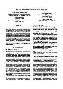
4.1. Properties of reflection domain clustering In the clustering of the TFLPCC, we use the reflection domain coefficients instead of LPC domain coefficients. The reflection domain coefficients have several advantages compared to the LPC domain coefficients [9]. Some of the advantages are: 1) the all pole filter is stable under perturbation provided that the corresponding reflection coefficients all lie between -1 and +1, 2) interpolating between two of reflection coefficients yields a smooth change in the frequency response. Figure 8 shows how the frequency response changes when we scale the reflection domain coefficients. The first plot is the frequency response of a time domain reflection coefficients. The second plot is the frequency response of the normalization of the coefficients whose norm is 1. The last plot is the frequency response of scale factor 0.01 multiplies the original coefficients. The figure shows that when the maximum component of reflect coefficient vector is much smaller than 1, rescaling the coefficient vector does not change the frequency response of the LPCC much. In other words, such a change in the frequency response is acceptable

Figure 5: TFLPC Synthesis

Figure 6: Time domain residue (above) and recovered excitation signal (below). Here we plot 7 overlapping frames to show the structure of one event.

coefficients to get the excitation signal in the time domain. Figure 6 shows the residue and the regenerated excitation in time domain. FDLPC captures the sub-frame contour shape well. Then we filter the time domain excitation using the TDLPC filter to get the time domain frame signal. 5) Repeat step 4 for all the frames inside one event and then overlap and add to reconstruct the event. 6) Repeat 2-5 until we generate events for all the event positions. 7) Mix the synthesized events and the background sound together to get the final result. The result is shown in Figure 7.

Figure 7: Sample sound (above) and regenerated sound (below).

4. EVALUATION AND DISCUSSION Informal listening tests show that the regenerated sound is quite similar to the sample audio clip. By using frame level contour extraction and TFLPC analysis, both the spectral and fine temporal characteristics of the sound are captured. To listen to and compare the original sound with the generated one, see our website http://www.zwhome.org/~lonce/Publications/da fx2004.html The error for each generated transient event comes from two sources: one is the error between the excitation signal and the original residue; another is the difference between the generated LPCC and the original one due to the clustering. It is not easy to quantitively measure the dissimilarity between the generated sound and the sample audio principally due to the statistical variation in the model.

348

DAFX-4

Figure 8: Scale effect of reflection LPC coefficients.

— DAFx'04 Proceedings —

348

th Proc. of of the the 77th Int.Conference Conferenceon onDigital DigitalAudio AudioEffects Effects(DAFx'04), (DAFX-04),Naples, Naples,Italy, Italy, October 5-8, 2004 Proc. Int. October 5-8, 2004

and our clustering algorithm can be independent of the vector magnitude. 4.2. Comparison with Other Methods

4.2.1. An HMM Method In the framework in Section 3, we cluster the reflection domain TDLPCC and FDLPCC into clusters separately and record the TDLPCC and FDLPCC cluster index sequences for each event to preserve the original order of the frames. By such a clustering we get two “codebooks” of the TDLPCC and FDLPCC separately and greatly reduce the amount of information in reconstruction. However preserving the specific cluster number sequence for each event also restricts the flexibility of modeling. To gain more flexibility, we train a Gaussian Mixture Model to capture the order pattern. After we get the reflection domain TDLPCC and FDLPCC sequence for each event as we do in Section 3, we use these TDLPCC sequences and FDLPCC sequence of all events to train two Gaussian mixture HMMs for TDLPC and FDLPC separately. In resynthesis, we use these two HMMs to generate the reflection domain TDLPCC sequence and FDLPCC sequence for regenerated events. However, result shows that such a system does not work well. In the Gaussian Mixture HMM, there are several possible Gaussian distributions for each state. When we generate coefficient vectors using the HMM, these distributions are chosen according to some probability. The randomness in the cluster sequence has a significant detrimental affect on the perceptual quality of the regenerated sound.

4.2.2. Comparison with Event-Based Method As another approach to reduce the amount of data, we implement a system using TFLPC analysis to entire events instead of overlapped frames. First the energy of each frame is calculated and then we extract events from the energy sequence of the whole sound as we do to the gain sequence in Section 3.2. Next we apply TFLPC analysis to individual events instead of frames so that we have only one TDLPCC vector and one FDLPCC vector for each event compare with frame-based method’s two vector sequences. The data amount is further reduced. However, there is a dramatic quality decrease when the event length is long. The reasons are as follows: 1) When the event length increases, the modeling ability of LPC decreases. We can use a greater filter order, but the quality is still worse than the short window case, 2) The limited amount of data affects the parameter extraction for the Gaussian distribution of each cluster. We get only two LPC vectors for each event instead of two LPC coefficient vector sequences, so there is not enough data to estimate the proper Gaussian distribution parameters for each cluster. Based on these reasons, among the several methods we implemented in our experiment, the frame-based TFLPC analysis method which is introduced in the system framework section worked the best. 5. FUTURE WORK We have demonstrated a method for modeling certain classes of sound textures. The method involves analysis at different time

349

scales to preserve perceptually relevant information for synthesis and resynthesis. Future work will focus on improvement of quality and generalization of this method to a wider class of sounds. Currently we use a frame-based TFLPC analysis. If we could capture the order pattern of the frames inside events, we could build pattern models to gain more flexibility. In the current system we assume all the events are of the same kind and use a single Poisson distribution to simulate the occurrence of the events. This assumption may be violated for some sounds, such as the sound from tennis game containing the players’ footstep sound and the driving-ball sound. By classifying the events into different classes and using different statistical distributions for sequencing them, we can build a better model for the sounds containing more than one kind of event. Some sounds with both broadband noise and densely-packed micro-transients are very difficult to segment into individual transient events from the residual information. It is difficult to get global statistical features such as event density to control the resynthesis and the frame by frame method loses flexibility. Segmentation of such complex sounds should also be explored to generalize this method for flexible resynthesis. 6. REFERENCES [1] E. Scheirer, B. Vercoe, “SAOL: The MPEG-4 Structured Audio Orchestra Language,” Computer Music Journal, vol. 23, no. 2, pp. 31−51, 1999. [2] L. Wyse, Y. Wang, X. Zhu, “Application of a Content-based Percussive Sound Synthesizer to Packet Loss Recovery in Music Streaming,” in Proc. of 11th ACM International Conference on Multimedia (Berkeley, CA), pp. 335−339, 2003. [3] J. Herre and J. D. Johnston, “Enhancing the Performance of Perceptual Audio Coders by Using Temporal Noise Shaping (TNS),” in Proc. 101st AES Conference., Nov 1996. [4] G. Tzanetakis, P. Cook, “Musical Genre Classification of Audio Signals,” IEEE Trans. on Speech and Audio Processing, vol. 10, no. 5, July 2002. [5] S. Dubnov, Z. B. Joseph, R. E. Yaniv, D. Lischinski, M. Werman, “Synthesizing sound textures through wavelet tree learning,” IEEE CGA, vol. 22, no. 4, pp. 38−48, Jul/Aug 2002. [6] N. St. Arnaud, K. Popat, “Analysis and synthesis of sound textures,” in Proc. AJCAI Workshop on Computational Auditory Scene Analysis, 1995. [7] W. H. Warren, R. R. Verbrugge, “Auditory Perception of Breaking and Bouncing Events: Psychophysics,” Natural Computation, W. Richards, Ed., pp. 364−375. MIT Press, 1988. [8] M. Athineos, D. P. W. Ellis, “Sound texture modeling with linear prediction in both time and frequency domains,” in Proc. of Int. Conf. on Acoustics, Speech, and Signal Processing, 2003. [9] B. S. Atal, P. V. Cox, P. Kroon, “Spectral quantization and interpolation for CELP coders,” Int. Conf. on Acoustics, Speech, and Signal Processing, May 1989. [10] M. Halkidi, Y. Batistakis, M. Vazirgiannis, “On Clustering Validation Techniques,” Journal of Intelligent Information Systems, 2001.

DAFX-5

— DAFx'04 Proceedings —

349